Printed version ISSN 0001-3765 / Online version ISSN 1678-2690 http://dx.doi.org/10.1590/0001-3765201620160232
www.scielo.br/aabc
Ecohydrological modeling and environmental flow regime in the Formoso River,
Minas Gerais State, Brazil
HUGO A.S.GUEDES1, DEMETRIUS D.SILVA2, JORGE A.DERGAM3
and ABRAHÃO A.A.ELESBON4
1
Centro de Engenharias, Universidade Federal de Pelotas/UFPEL, Rua Benjamim Constant, 989, Simões Lopes, 96010-020 Pelotas, RS, Brazil
2
Departamento de Engenharia Agrícola, Universidade Federal de Viçosa/UFV, Avenida PH Rolfs, s/n, Campus Universitário, 36570-000 Viçosa, MG, Brazil
3
Departamento de Biologia Animal, Universidade Federal de Viçosa/UFV, Avenida PH Rolfs, s/n, Campus Universitário, 36570-000 Viçosa, MG, Brazil
4
Instituto Federal de Educação, Ciência e Tecnologia do Espírito Santo, Avenida Arino Gomes Leal, 1700, 29700-660 Colatina, ES, Brazil
Manuscript received on April 27, 2016; accepted for publication on August 12, 2016
ABSTRACT
This paper aimed at determining the environmental flow regime in a 1 km stretch of the Formoso River,
MG, using River2D model. To carry out the ecohydrological modeling, the following information was used: bathymetry, physical and hydraulic features, and the Habitat Suitability Index for species of the Hypostomus auroguttatus. In the River2D, the Weighted Usable Areas were determined from the average
long-term streamflows with percentage from 10% to 100%. Those streamflows were simulated for the
later construction of optimization matrices that maximize the habitat area throughout the year. For H. auroguttatus Juvenile, higher values of Weighted Usable Area were associated with the percentage of
60% and 70% of the average long-term streamflows in October and September, respectively. For H. auroguttatus Adult, the highest value of Weighted Usable Area was associated with the percentage of
100% of the average long-term streamflow in September. The environmental flows found for this stretch of the Formoso River varied over the year. The lowest environmental flow was observed in December
(2.85 m3 s-1), while the highest was observed in May (4.13 m3 s-1). This paper shows the importance of ecohydrological studies in forming a basis for water resources management actions.
Key words: ecohydrology, hydrodynamic modeling, River2D, water resources, WUA.
Correspondence to: Hugo Alexandre Soares Guedes E-mail: [email protected]
INTRODUCTION
The need for drinking water and the dependency
on ecological goods and services sustained by fluvial ecosystems represent a big challenge to water resources managers (Arthington et al. 2010). Nowadays, multiple forms of water use generate
conflicts, making pressure on water resources. In
order to relieve this pressure, several programs for water resources management are proposed. Those
seek to discipline water use, making quantitative and qualitative aspects become compatible with the
development of ecosystems and human activities both (Almeida et al. 2014, Castro et al. 2016).
promote the balance between multiple uses of water, granting the right to use water resources. The permit allows the entity that manages water resources to determine the amount of water that can
be available in a stream as well as the streamflow that keeps the integrity of aquatic communities. This streamflow is known as remaining streamflow
(Castro et al. 2016). Although having a characteristic of preservation, the remaining streamflow does not demonstrate the real situation of a stream. It
does not consider the necessities of aquatic species according to streamflow variations that rule food
availability, reproduction and the physical features
of the habitat (Huckstorf et al. 2008, Guedes et al.
2014, Kolden et al. 2016).
Through the analysis of hydrological and ecological variables ecohydrological studies try to establish an environmental flow regime that considers the natural hydrological variations of a
river. Since aquatic species are adapted to them and
depend on them to carry out their vital functions
(Zalewski 2002, 2015, Arthington et al. 2006).
Environmental flow is a term proposed to conciliate water resources forms of use with the
need of conservation of an aquatic ecosystem, a
necessary process in order to maintain sustainable
fluvial ecosystems (Wang et al. 2013). Thus, the environmental flow must be analysed according to
its seasonal variability. It is necessary to determine
the monthly flow regime to be kept in the stream so as to guarantee the aquatic biodiversity (Souza et
al. 2008a).
Habitat classification method is the most
complete to evaluate the environmental flow. They
contemplate several steps, such as physical and environmental features, study plan elaborated by a multidisciplinary team, and different types of analysis (Benetti et al. 2003). This method may consider economic aspects, evaluating the willing to pay for the environmental preservation and
the benefits generated by water permit, pursuing the best quantification for an environmental flow
(Souza et al. 2008a).
Increasing expansion of demands makes the
water resources management associated with the ecological integrity maintenance become more
and more complex, since the environmental flows
must attend to anthropic and ecological demands simultaneously (Richter et al. 2003). Due to the
complexity of applying the knowledge acquired
along these years, mathematical models are an
important tool for supporting decision making
systems. They allow to test alternative scenarios and to implement ecohydrological methodologies aiming at the management of sustainable water and
ecosystems uses (Zalewski 2010).
Advances in environmental modeling provide tools to represent the complex interactions between
fish populations and their habitats, pursuing to re -late several features of a river stretch, such as ve-locity, depth, and substrate to habitat preferences of certain species or groups of species (Boavida et al. 2011). According to Govind et al. (2009), cou-pling ecosystem models with hydrological models is a research direction for future ecohydrological studies.
In those studies, unidimensional models that only describe spatial variations along a direction are
frequently used. Differently from unidimensional
models, hydrodynamic modeling in two dimensions
shows a better final result, since it represents with
accuracy spatial and timing variations (Jowett and Duncan 2012).
Among the different bidimensional softwares
used in ecohydrological modeling, River2D
(Steffler and Blackburn 2002) stands out due to its use in studies to determine environmental flows
and to establish the ecological hydrogram (Sanz and Martínez 2008, Polo and Torres 2009), to revitalize rivers (Jalón and Gortázar 2007, Boavida et al. 2011), and to study the habitat with a view to protecting endangered species (Parasiewicz et al. 2012), among others.
However, few researches about the
-sional modeling are carried out in Brazil (Guedes et al. 2014, Castro et al. 2016). Having this in mind, this paper aimed at determining the environmental
flow regime in the Formoso River, MG, using the
bidimensional model River2D.
MATERIALS AND METHODS
STUDY SITE
This study was carried out in the Formoso River,
tributary on the right bank of the Pomba River,
located in the West part of the Paraíba do Sul River basin, Brazil Southeast region (Figure 1), which is
76.7 km long. The Formoso River basin has an area of approximately 398 km². The studied stretch is
located at the lower part of the basin, corresponding to a degraded area, since its native vegetation was suppressed due to intensive use for pasture. Withdraw of this vegetation accelerated the erosion
process on the banks of the river, increasing the
concentration of sediments in the stream. Besides,
there is the throwing of sanitary effluents without
treatment coming from the population that lives
near the river, deeply degrading the fluvial system.
Physical, hydraulic, and habitat
characteriza-tions were done in a stretch of 1 km long of the For
-moso River. Three equidistant transversal sections
of 500 meters from one border to the other were delimited and information about velocity, depth,
discharge, fishes and substrate was collected.
PHYSICAL AND HYDRAULIC CHARACTERIZATION
The physical characterization of the river stretch was done based on the bathymetry survey, which
employed geodetic GPS Promark II and a Total
Station Topcon GTS 212. Exactly 1879 points were
tracked by the geodetic GPS, allowing the work’s
georeferencing.
Substrate collection was done in each transversal section using a vertical penetration Petersen dredge with collecting capacity of 3.20 liters. Materials collected were analysed at the Laboratório de Propriedades Físicas do Solo, of the Departamento de Solos, of the Universidade Federal de Viçosa. Their granulometry and their mean particle diameter were measured (Jalón and Gortázar 2007).
Depth (m), width (m), velocity (m s-1) and streamflow (m3 s-1) were measure during four periods, twice in the dry period (June, 2011 and July, 2012) and twice in the rainy period (March,
2011 and February, 2012). Streamflow measured
in the beginning stretch of the river were: 7.52 m3 s-1 (03/26/2011), 5.97 m3 s-1 (06/18/2011), 10.25 m3 s-1 (02/11/2012) and 5.75 m3 s-1 (07/07/2012).
Velocity was monitored during the two first periods
using a very small hydraulic windlass M1 by SEBA Hydrometrie®. On the third period, due to a bigger
magnitude of streamflow, velocity was monitored
by a Newton fluviometric windlass by Hidromec®.
On the fourth period the ADCP – Acoustic Doppler Current Profiler, model M9 RiverSurveyor by
Sontek® was used. The depth was measured from
the bathymetry of the transversal sections.
HISTORICAL SERIES OF STREAMFLOW
The historical series of streamflow gauging sta
-tion (Tabuleiro, code 58720000), with 23 years of
daily streamflow data, was used to obtain the daily
streamflow. The average long-term streamflows were obtained by software SIsCAH (Sousa et al.
2009), allowing the analysis of the runoff regime
in the basin.
HABITAT SUITABILITY INDEX
The Habitat Suitability Index (HSI) is represented as a function of the curves for the Habitat Suitability Criteria (HSC). It represents the level of preference
that a fish has in relation to the abiotic variables
of depth, velocity, and substrate (Lee et al. 2010, Chou and Chuang 2011).
This study analysed the species Hypostomus auroguttatus Kner, 1854 (Pisces, Loricariidae), for they are representative of the Formoso River (Guedes et al. 2014). They prefer habitats with fast (velocity faster than 0.8 m s-1) and coarse substrate (rugosity bigger than 0.35 m) (Casatti et al. 2005).
The HSI preference curves were obtained according to the methodology proposed by Chou and Chuang (2011), performed by Castro et al. (2016),
considering the frequency and the preferences of the
species studied for depth, velocity, and substrate.
The weighted frequency of the preference curve
was determined from the relationship between the number of individuals collected in each class of variables observed (velocity, depth, and substrate) and the total number of individuals collected during
the monitoring. The frequencies of the variables were divided according to the greatest frequency obtained, making HSI a weighted index.
The substrate was analysed considering the features of the channel and it was used in the mod-eling to determine the habitat preference among the bioindicator species. The following information was considered: silt (code 1), sand (code 2), gran-ule (code 3), pebble (code 4), cobble (code 5 or 6),
boulder (code 7 or 8), rocky bed (code 9), and bank
with vegetation (code 10) (Bovee 1982).
The HSI preference curves were elaborated according to the development stage (adult and
juvenile) taking into account each variable as well
as the area use by the species. Thus, they permitted to determine the species habitat preference (Chou and Chuang 2011), which ranged from 0 (inappropriate) to 1 (optimal) (Bovee 1982).
MODEL RIVER2D
The model River2D was chosen to this study
because it is the most efficient model in terms of
such as habitat quality for fishes, compared to unidimensional models (Brown and Pasternarck
2009, Lee et al. 2010).
River2D consists in a bidimensional model, developed specifically to be used for rivers or natural streams, based on the Finite Element Method and on the conservative formulation by
Petrov-Galerkin (Steffler and Blackburn 2002).
In the computational modeling the model River2D and its modules: RiverBed (R2D_ Bed), RiverMesh (R2D_Mesh) as well as the hydrodynamic component River2D were used. The topographical editing was carried out in R2D_Bed, in which the bathymetric data were annotated; these were processed in the computer programs AutoCAD 2011. The post-processing of bathymetric data, such as the geographical
correction of points obtained in field, took place in
the program ESRI ArcGis 10. Later, bathymetric data were interpolated into every studied stretch using the module R2D_Bed.
In R2D_Mesh, the mesh of finite elements was created and the boundary conditions were defined, corresponding to the streamflow in the section at
the entrance of the stretch of 7.52 m3 s-1. The lateral boundary conditions were defined as without
runoff.
Verification of the calibration in the R2D_ Mesh module is done considering the Quality Index (QI). This index is defined according to the ratio of the area of each triangle of the mesh to its circumscribed circumference. Satisfactory
values of refinement are represented as QI with values between 0.1 and 0.5 (Waddle and Steffler
2002). To reach these values it was necessary to do successive operations of edition and to change the values of roughness of the riverbed. In this study,
the integration step used was equal to 1 minute, presenting a time of simulation equal to 2 minutes as well as a mistake associated of 0.00006. Thus,
the value found for QI was 0.10. This generated a mesh with mean resolution of 5.0 m.
Validation of the calibration for depth and velocity was done considering the Mean Absolute
Error (MAE) and Root Mean Square Error (RMSE)
between the measured and the simulated values, as proposed by Lacey and Millar (2004) and Chou and Chuang (2011).
After the calibration of the model River2D
was concluded and verified, it was used to simulate the different scenarios for the streamflows using the percentage of 10% to 100% of average long-term
streamflows. Thus the maximum environmental
flow to be reached would be the natural flow regime
(Guedes et al. 2014).
HABITAT MODELING
The component habitat of River2D model is based on the Weighted Usable Area – WUA, proposed by
Bovee (1982). The WUA is the quantity of physical habitat available, expressed in square meters per kilometer of a stream for the fish species in a streamflow (Eq. 1).
(
)
1
,
,
.
n
i i i i
i
WUA
f V P S
A
=
é
ù
=
å
ë
û
(1)where Ai is the area of the stream in each cell i [L2]; Vi is the velocity in each cell [LT-1]; Pi is the depth in each cell [L]; Si is the effective roughness (ks) of the substrate in each cell [L]; and f (Vi, Pi, Si) is the suitability index combined with the area Ai [L].
The WUA is calculated using the HSI pref-erence curves evaluated in each point of domain (computational nodes of the discretized mesh). And also in each point of the usable surface (Thiessen
Polygons) associated to it (Steffler and Blackburn
2002).
The WUA was calculated using H. aurogutta-tus juveniles as well as adults preference curves re-garding the variables depth, velocity, and substrate, using the geometric mean between the suitability
indexes (Steffler and Blackburn 2002, Guedes et
associated with the average long-term streamflows
used in the simulation, supporting the estimate of
the environmental flow regime.
ENVIRONMENTAL FLOW REGIME
Determination of the environmental flow regime
must consider the magnitude, the duration and
the frequency of streamflows in a stream (Poff
and Zimmerman 2010). In this study, the monthly environmental flow was estimated through the optimization matrix proposed by Bovee (1982).
The optimization matrix consists of the con-struction of a matrix for each month of the year.
Columns correspond to the simulated streamflow
and lines to the species considered in the study
(Bo-vee 1982). To each simulated streamflow it is cal
-culated a value of WUA using the model River2D. The highest is the value, the highest is the suitabil-ity of a species in the studied stretch.
Monthly environmental flow was determined
as follows: after calculating the WUA for each
simulated streamflow each column was analysed.
The minimum value of WUA was selected and registered in the last line of the matrix. The highest level of this line was highlighted. This value corresponds to the poorliest simulated value in the stream in order to guarantee the maintenance of the most vulnerable species in the studied stretch.
This streamflow corresponds to the environmental flow. This process was repeated for each month of
the year (Bovee 1982, Guedes et al. 2014, Castro et al. 2016).
RESULTS AND DISCUSSION
In the calibration of the River2D, the finite elements
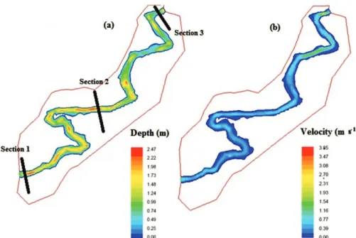
mesh presented 9326 nodes, 18182 elements and 68 interactions. Depth and velocity distributions
are presented in Figure 2. The streamflow used in the calibration was equal to 7.52 m3
s-1.
Depth ranging from 0.75 m to 1.00 m (Figure
2a) was found in 19% of the studied stretch and
values above 2.00 m was found in 9% of it. Depth
values lower than 0.75 m were found between monitoring sections 2 and 3. They can be related to the strong degradation and to the conditions of siltation in the stream. According to Faria et al. (2013), erosion processes due to siltation lead to degradation of water resources and diminish the depth of streams.
Regarding velocity (Figure 2b), 61% of the
studied stretch showed values ranging from 0.10 m s-1 to 0.50 m s-1 justified by the flat terrain. Velocity above 2.00 m s-1 was found in 11% of the stretch located between the sections 2 and 3, exactly the same stretch with the lowest depth. This indicates the torrential regime in the stream (Mejía 2008).
These simulations were frequently observed during the monitoring in field, proving River2D
precision in determining the interaction between
the streamflows in rivers and the bathymetry of
the channel. Similar observations were done by Boavida et al. (2012) and Castro et al. (2016).
The MAE calculated for depth in the
transversal sections was 5.4%, while the MAE for velocity was 13.4%. The RMSE obtained for depth
in the transversal sections was 0.079 m, and the RMSE for velocity was 0.159 m s-1. The difference between the transversal sections considered in the
Rive2D can influence the adjustment between the
simulated and the observed values of the hydraulic
variables, since the composition of the area by finite
elements method generates softer surfaces than the
ones measured in field (Boavida et al. 2013).
Jowett and Duncan (2012) found MAE of
22% and 34% for depth and velocity, respectively.
According to these authors, River2D tends to underestimate the depth values, and depending
on the flow conditions, it may underestimate or
riverbed features. Despite these discrepancies, the authors highlighted the importance of River2D in simulating the physical environment conditions.
The table for simulated WUA and average long-term streamflows associated with the
percentage from 10% to 100% in the studied stretch
are presented in Table I. An analysis of Table I shows that the WUA values varied between life
stages and among the different months according to the average long-term streamflows. A similar result
was found by Guedes et al. (2014) and Castro et al. (2016).
Figure 2 - Formoso River stretch studied. a. Depth. – b. Velocity.
TABLE I WUA, m2
km-1, and the average long-term streamflows associated with the percentage of 10 to 100% in the Formoso River
stretch studied.
H. auroguttatus
JANUARY (Qmean = 17.25 m 3 s-1
)
Percentage of 10 to 100% of the average long-term streamflow x WUA (m2 km-1 )
10 20 30 40 50 60 70 80 90 100
Juvenile 14.16 23.39 19.79 7.78 4.18 2.22 4.16 3.98 4.36 6.41
Adult 44.16 102.15 107.88 67.95 44.63 33.13 53.63 46.58 48.78 50.85
Minimum of the column 14.16 23.39 19.79 7.78 4.18 2.22 4.16 3.98 4.36 6.41 Maximum of the minima WUA: 23.39 m2
km-1 Environmental flow: 3.45 m3 s-1
FEBRUARY (Qmean = 12.75 m 3 s-1
)
Juvenile 7.72 16.43 23.25 12.27 9.71 6.04 3.13 2.94 2.42 8.22
Adult 19.81 67.18 101.88 87.84 78.71 56.94 38.98 35.24 31.28 57.70
Minimum of the column 7.72 16.43 23.25 12.27 9.71 6.04 3.13 2.94 2.42 8.22 Maximum of the minima WUA: 23.25 m² km-1 Environmental flow: 3.83 m³ s-1
MARCH (Qmean = 12.06 m 3 s-1
)
Juvenile 9.06 16.01 24.28 14.78 10.70 6.91 4.11 2.77 2.80 4.73
Adult 23.93 64.98 102.15 93.33 84.43 62.4 44.73 36.08 34.21 40.41
APRIL (Qmean = 8.58 m 3 s-1
)
Juvenile 2.10 14.16 16.98 24.79 20.47 12.20 10.72 8.16 5.64 4.29
Adult 4.79 44.16 69.47 100.54 102.73 87.61 84.57 70.16 54.28 45.81
Minimum of the column 2.10 14.16 16.98 24.79 20.47 12.20 10.72 8.16 5.64 4.29 Maximum of the minima WUA: 24.79 m² km-1 Environmental flow: 3.43 m³ s-1
MAY (Qmean = 6.89 m 3 s-1
)
Juvenile 0.49 9.58 13.00 18.13 17.04 21.57 14.78 10.89 10.43 9.28
Adult 0.83 25.34 49.13 74.22 68.61 103.78 93.33 85.61 82.69 76.49
Minimum of the column 0.49 9.58 13.00 18.13 17.04 21.57 14.78 10.89 10.43 9.28 Maximum of the minima WUA: 21.57 m² km-1 Environmental flow: 4.13 m³ s-1
JUNE (Qmean = 5.42 m 3 s-1
)
Juvenile 0.16 3.77 11.89 13.32 18.56 22.56 23.44 19.17 14.38 14.09
Adult 0.12 9.15 35.55 51.20 75.64 91.65 101.88 100.49 92.63 90.77
Minimum of the column 0.12 3.77 11.89 13.32 18.56 22.56 23.44 19.17 14.38 14.09 Maximum of the minima WUA: 23.44 m² km-1 Environmental flow: 3.79 m³ s-1
JULY (Qmean = 5.10 m 3 s-1
)
Juvenile 0.16 4.88 11.74 13.09 16.43 23.29 24.69 22.39 16.32 12.27
Adult 0.12 12.19 33.77 49.84 66.54 93.33 102.61 104.03 95.22 87.84
Minimum of the column 0.12 4.88 11.74 13.09 16.43 23.29 24.69 22.39 16.32 12.27 Maximum of the minima WUA: 24.69 m² km-1 Environmental flow: 3.57 m³ s-1
AUGUST (Qmean = 4.66 m 3 s-1
)
Juvenile 1.71 1.91 10.28 12.36 15.98 20.06 18.11 23.74 21.17 17.50
Adult 1.62 3.96 28.25 42.23 64.69 81.27 76.30 99.88 103.41 94.44
Minimum of the column 1.62 1.91 10.28 12.36 15.98 20.06 18.11 23.74 21.17 17.50 Maximum of the minima WUA: 23.74 m² km-1 Environmental flow: 3.73 m³ s-1
SEPTEMBER (Qmean = 5.06 m 3 s-1
)
Juvenile 0.16 4.88 11.74 13.07 16.47 23.28 25.42 22.38 16.99 21.24
Adult 0.12 12.19 33.78 49.76 67.38 93.31 103.78 104.30 96.08 113.09
Minimum of the column 0.12 4.88 11.74 13.07 16.47 23.28 25.42 22.38 16.99 21.24 Maximum of the minima WUA: 25.42 m² km-1 Environmental flow: 3.54 m³ s-1
OCTOBER (Qmean = 5.91 m 3 s-1
)
Juvenile 0.16 7.79 12.18 16.00 21.64 25.42 21.30 15.50 11.00 13.19
Adult 0.12 20.04 39.73 64.86 87.34 103.78 103.51 94.02 85.56 81.81
Minimum of the column 0.12 7.79 12.18 16.00 21.64 25.42 21.30 15.50 11.00 13.19 Maximum of the minima WUA: 25.42 m² km-1 Environmental flow: 3.55 m³ s-1
NOVEMBER (Qmean = 9.63 m 3 s-1
)
Juvenile 2.46 12.54 20.78 23.13 14.78 10.64 8.44 5.64 3.60 4.19
Adult 5.68 44.43 84.07 102.17 93.33 85.13 71.66 54.27 41.82 39.61
Minimum of the column 2.46 12.54 20.78 23.13 14.78 10.64 8.44 5.64 3.60 4.19 Maximum of the minima WUA: 23.13 m² km-1 Environmental flow: 3.85 m³ s-1
DECEMBER (Qmean = 14.26 m 3 s-1
)
Juvenile 10.53 20.88 20.47 10.72 7.35 4.32 2.81 2.42 8.22 3.94
Adult 28.47 84.35 102.73 85.42 65.31 45.85 35.59 33.98 57.70 47.42
Minimum of the column 10.53 20.88 20.47 10.72 7.35 4.32 2.81 2.42 8.22 3.94 Maximum of the minima WUA: 20.88 m² km-1 Environmental flow: 2.85 m³ s-1
For H. auroguttatus Juvenile, WUA higher
values are associated with the percentage of 60% and 70% of the average long-term streamflows
in October and September, respectively. For H. auroguttatus Adult, WUA highest value is associated
with the percentage of 100% of the average
long-term streamflow in September. October and September correspond to the dry season end in the Formoso River. This shows a preference of H. auroguttatus for lower streamflows, confirming the
results found by Castro et al. (2016). According to Leal et al. (2013) individuals tend to occupy the habitats where they are most adapted to. So, the relation between species and certain environmental variables, such as velocity, depth, discharge and substrate is usually intense.
But WUA higher values only do not guarantee greater abundance of H. auroguttatus individuals, since the permanence in the stream depends on oth-er factors, such as food availability (Condini et al. 2011). According to Dunham et al. (2003) although River2D disregards other ecological factors that
have a significant impact on Hypostomus
popula-tion, such as the presence of pre-existent or exotic species, habitat connectivity, and food availability,
it reflects this species’ population dynamics.
According to Ferreira and Casatti (2006), among the factors that affect the icthyofauna distribution in lotic environments, loss and transformation of internal habitat stand out. They are usually associated with the riparian forest
suppression and to the consequent rise of the solar
incidence as well as the absence of certain food
items, like fruits, seed and allocthone insects (King
and Warburton 2007, Mouton et al. 2012). These features are found all along the studied stretch of the Formoso River, justifying lower WUA values compared to the study done by Castro et al. (2016).
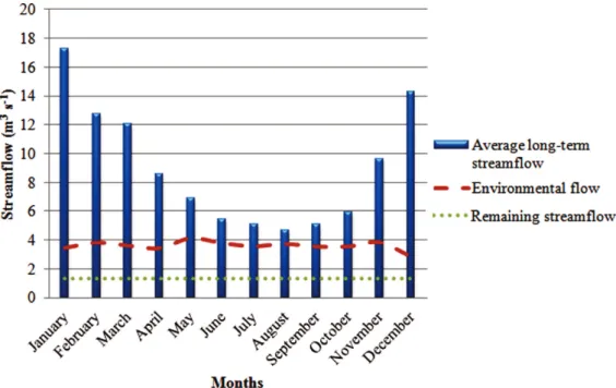
Figure 3 shows the environmental flow regime
for the studied stretch of the Formoso River, as well
as the remaining streamflow. It corresponds to 50% of the seven days long minimum streamflow with a
return period of ten years – Q7,10, the same scenario considered by the Instituto Mineiro de Gestão das Águas (IGAM) in this part of Minas Gerais state for analyses of water right permits.
Figure 3 - Environmental flow regime, average long-term streamflows, and remaining streamflow for the
The environmental flows found for the Formoso
River stretch varied along the year. The lowest environmental flow was observed in December (2.85 m3 s-1), while the highest was observed in May (4.13 m3 s-1). In May, a characteristic month of the dry period in the Formoso River basin, the
environmental flow tends to be higher due to the
need of maintenance of the ecological integrity of the stream. December, a characteristic month of the
rainy period that naturally presents the streamflows
more elevated in the river basin has a water supply
that keeps the physical habitat of the species. So
it is not necessary to maintain a higher level of
environmental flow. Note that this is a preliminary
analysis and that the definition of the monthly
environmental flow should be done considering the
necessities of use of water resources in the river basin (Souza et al. 2008b).
H. auroguttatus Juvenile was the most
sensi-tive to streamflow variation, since it presented the
lowest value of WUA. Thus, this species limited
the environmental flow definition in the Formoso
River degraded stretch. Therefore, the
environ-mental flow regime established guarantees the sus
-tainability and the minimum environmental condi-tion in order to maintain the species in the studied stretch.
The streamflows represent the main force be
-hind freshwater ecosystems, determining the
dis-tribution, the abundance, and the river organisms’
diversity (Poff et al. 1997, Santos et al. 2010).
Streamflow reduction to a lower rate than a value considered minimum to the environmental flow in
a stream does not necessarily extinguish certain species. However, it can cause the individuals mov-ing to other sites of the river or even to tributar-ies with similar suitability features, since there is
aquatic ecosystems interrelation. These species can come back to their original stream when conditions
become favorable again.
Comparing the current criterion of water use permits in Minas Gerais state with remaining
streamflow (Figure 3) and with the environmental flow in December (most critical month) it can be
concluded that the species would probably move to other river stretches, or even to the nearest tributaries that present higher streamflows and better suitability conditions. Thus, this Formoso River stretch can present fish species reduction
since environmental flow values are much higher than the remaining streamflow established by the
current permit criterion of surface water.
According to Postel and Richter (2003) fixing
a value of environmental flow for a stream can
damage the aquatic fauna since the environmental flow has space and time variation. Furthermore, environmental effects that happen in the aquatic habitat are associated with the different environment
regime levels, not only because of a streamflow
minimum value, but also because of the streamflows
medium and maximum values, besides the features of the hydrologic regime, such as duration and
frequency of extreme events. According to Escobar
(2008), the biological productivity and diversity
of the fluvial ecosystems are guaranteed if these
features are present.
Environmental flow values should not be adopted only based on the results obtained. This paper consists in the initial process of an attempt to
find an environmental flow regime effectiveness. So it is necessary several presentations of workshops to
agencies and basin committees, to water users and mainly to the civil society before implementing it.
CONCLUSIONS
Environmental flows found for the Formoso River stretch varied all over the year. The lowest environmental flow was observed in December (2.85 m3 s-1), while the highest was observed in May (4.13 m3 s-1). Comparing the current criterion of water use permits in Minas Gerais state to the remaining streamflow and to the environmental
concluded that the species would probably move to other river stretches, or even to the nearest tributaries that present higher streamflows and better suitability conditions. This study shows the importance of ecohydrological studies in forming a basis for water resource management actions.
H. auroguttatus Juvenile was the species most
sensitive to streamflow variation, since it presented
the least values of WUA. Thus, this species limited
the environmental flow definition in the Formoso
River degraded stretch.
The methodology presented can be applied in
any river, without distinction of size and streamflows
magnitude. It should be emphasized that the bigger
the stream, the more exhaustive will be the field work. The greatest limitation of this methodology refers to the precise determination of fish groups to be considered in the environmental flow regime.
Besides, it demands a lot of experience from the experts and a certain subjectivity degree.
ACKNOWLEDGMENTS
The authors would like to thank the Fundação de Amparo à Pesquisa de Minas Gerais (FAPEMIG)
and the Conselho Nacional de Desenvolvimento
Científico e Tecnológico (CNPq) for the financial
support.
REFERENCES
ALMEIDA WA, MOREIRA MC AND DA SILVA DD. 2014. Applying water vulnerability indexes for river segments. Water Resour Res 28: 4289-4301.
ARTHINGTON AH, BUNN SE, POFF NL AND NAIMAN RJ. 2006. The Challenge of Providing Environmental Flow Rules to Sustain River Ecosystems. Ecol Appl 16: 1311-1318.
ARTHINGTON AH, NAIMAN RJ, McCLAIN ME AND NILSSON C. 2010. Preserving the biodiversity and ecological services of rivers: new challenges and research opportunities. Freshwater Biol 55: 1-16.
BENETTI AD, LANNA AE AND COBALSHINI MS. 2003. Current practices for establishing environmental flows in Brazil. River Res Appl 19: 1-18.
BOAVIDA I, SANTOS JM, CORTES RV, PINHEIRO AN AND FERREIRA MT. 2011. Assessment of instream
structures for habitat improvement for two critically
endangered fish species. Aquat Ecol 45: 113-124.
BOAVIDA I, SANTOS JM, CORTES RV, PINHEIRO AN
AND FERREIRA MT. 2012. Benchmarking river habitat
improvement. River Res Appl 28: 1768-1779.
BOAVIDA I, SANTOS JM, KATOPODIS C, FERREIRA MT AND PINHEIRO A. 2013. Uncertainty in predicting the fish-response to two dimensional habitat modeling using field data. River Res Applic 29: 1164-1171.
BOVEE KD. 1982. A guide to stream habitat analysis using the instream flow incremental methodology. Instream Flow Information Paper No. 12. Fort Collins: U.S. Fish and Wildlife Service, 273 p.
BROWN RA AND PASTERNACK GB. 2009. Comparison of methods for analysing salmon habitat rehabilitation designs for regulated rivers. River Res Appl 25: 745-772. CASATTI L, ROCHA FC AND PEREIRA DC. 2005. Habitat
use by two species of Hypostomus (Pisces, Loricariidae) in southeastern Brazilian streams. Biota Neotrop 5: 1-9. CASTRO ERRS, MOREIRA MC AND SILVA DD. 2016.
Environmental flow in the River Ondas basin in Bahia, Brazilian Cerrado. Environ Monit Assess 188: 68-77. CHOU W-C AND CHUANG M-D. 2011. Habitat evaluation
using suitability index and habitat type diversity: a case study involving a shallow forest stream in central Taiwan. Environ Monit Assess 172: 689-704.
CONDINI MV, SEYBOTH E, VIEIRA JP AND GARCIA
AM. 2011. Diet and feeding strategy of the dusky grouper
Mycteroperca marginata (Actinopterygii: Epinephelidae)
in a man-made rocky habitat in southern Brazil. Neotrop
Ichthyol 9: 161-168.
DUNHAM JB, YOUNG M, GRESSWELL RE AND RIEMAN BE. 2003. Effects of fire on fish populations: landscape perspectives on persistence of native fishes and nonnative fish invasion. For Ecol Manage 178: 183-196.
ESCOBAR YC. 2008. Environmental flow regime in the
framework of integrated water resources management
strategy. Ecohydrol Hydrobiol 8: 307-315.
FARIA TO, VECCHIATO AB, SALOMÃO FXT AND SANTOS JÚNIOR WA. 2013. Abordagem morfope-dológica para diagnóstico e controle de processos erosi-vos. Ambi-Agua 8: 215-232.
FERREIRA CP AND CASATTI L. 2006. Influência da estrutura do habitat sobre a ictiofauna de um riacho em uma micro-bacia de pastagem, São Paulo, Brasil. Rev Bras Zool 23: 642-651.
GOVIND A, CHEN JM, MARGOLIS H, JU W, SONNENTAG O AND GIASSON M-A. 2009. A spatially explicit
hydro-ecological modeling framework (BEPS-TerrainLab V2.0):
model description and test in a boreal ecosystem in Eastern North America. J Hydrol 367: 200-216.
ecológicas no Rio Formoso/MG com base em espécies neotropicais. Rev Bras Rec Híd 19: 72-82.
HUCKSTORF V, LEWIN W-C AND WOLTER C. 2008. Environmental flow methodologies to protect fisheries resources in human-modified large lowland rivers. River Res Appl 24: 519-527.
JALÓN DG AND GORTÁZAR J. 2007. Evaluation of stream habitat enhancement options using fish habitat
simula-tions: case-studies in the river Pas (Spain). Aquat Ecol 41:
461-474.
JOWETT IG AND DUNCAN MJ. 2012. Effectiveness of 1D and 2D hydraulic models for instream habitat analysis in a braided river. Ecol Eng 48: 92-100.
KING S AND WARBURTON K. 2007. The environmental preferences of three species of Australian freshwater fish in relation to the effects of riparian degradation. Environ Biol Fish 78: 307-316.
KOLDEN E, FOX BD, BLEDSOE BP AND KONDRATIEFF
MC. 2016. Modelling Whitewater Park Hydraulics and
Fish Habitat in Colorado. River Res Applic 32: 1116-1127. LACEY RWJ AND MILLAR RG. 2004. Reach scale hydraulic
assessment of instream salmonid habitat restoration. J Am Water Resour Assoc 40: 1631-1644.
LEAL CG, JUNQUEIRA NT, SANTOS HAE AND POMPEU PS. 2013. Variações ecomorfológicas e de uso de habitat em Piabina argentea (Characiformes, Characidae) da bacia do rio das Velhas, Minas Gerais, Brasil. Ilheringia, Sér Zool 103: 222-231.
LEE JH, KIL JT AND JEONG S. 2010. Evaluation of physical
fish habitat quality enhancement designs in urban streams
using a 2D hydrodynamic model. Ecol Eng 36: 1251-1259. MEJÍA FJ. 2008. Relación de las curvas de energia específica
y pendiente de fricción con las zonas de flujo libre en canales. EIA 9: 69-75.
MOUTON AM, BUYSSE D, STEVENS M, VAN DEN NEUCKER T AND COECK J. 2012. Evaluation of Riparian Habitat Restoration in a Lowland River. River Res Appl 28: 845-857.
PARASIEWICZ P, CASTELLI E, ROGERS JN AND PLUNKETT E. 2012. Multiplex modeling of physical habitat for endangered freshwater mussels. Ecol Model 228: 66-75.
P O F F N L , A L L A N J D , B A I N M B , K A R R J R , PRESTEGAARD KL, RICHTER BD, SPARKS RE AND STROMBERG JC. 1997. The natural flow regime: a paradigm for river conservation and restoration. BioScience 47: 769-784.
POFF NL AND ZIMMERMAN JKH. 2010. Ecological responses to altered flow regimes: a literature review to inform environmental flows science and management. Freshwater Biol 55: 194-205.
POLO JF AND TORRES JMH. 2009. El régimen de caudales mínimos en el nuevo ciclo de la planificación hidrológica. Aspectos metodológicos y procesos de concertación social. Ingen Territ 85: 46-55.
POSTEL S AND RICHTER B. 2003. Rivers for life: Manag-ing water for people and nature.Washington: Island Press, 253 p.
RICHTER BD, MATHEWS R, HARRISON DL AND WIGINGTON R. 2003. Ecologically sustainable water management: Managing river flows for ecological integrity. Ecol Appl 13: 206-224.
SANTOS ABI, TERRA BF AND ARAÚJO FG. 2010. Influence of the river flow on the structure of fish assemblage along the longitudinal gradient from river to reservoir. Zool 27: 732-740.
SANZ DB AND MARTÍNEZ DV. 2008. Estimación de cau-dales ecológicos en dos cuencas de Andalucía: uso conjun-to de aguas superficiales y subterráneas. Ecosist 17: 24-36. SOUSA HT, PRUSKI FF, BOF LHN, CECON PR AND SOU-SA JRC. 2009. SisCAH 1.0: Sistema Computacional para
Análises Hidrológicas. Grupo de Pesquisa em Recursos
Hídricos. Minas Gerais: Universidade Federal de Viçosa. SOUZA CF, AGRA S, TASSI R AND COLLISHONN W.
2008b. Desafios e oportunidades para a implementação do hidrograma ecológico. REGA 5: 25-38.
SOUZA CF, TASSI R, MARQUES D DA M, COLLISHONN W AND AGOSTINHO AA. 2008a. Ecohydrology Towards the Sustainable Development: An Approach Based on South American case studies. Ecohydrol Hydrobiol 8: 225-235.
STEFFLER P AND BLACKBURN J. 2002. Two-Dimensional Depth Averaged Model of River Hydrodynamics and Fish Habitat. Alberta: University of Alberta, 120 p.
WADDLE T AND STEFFLER P. 2002. R2D_Mesh. Mesh generation program for River2D two dimensional depth averaged finite element. Introduction to mesh generation
and user’s manual. Fort Collins, EUA: U.S. Geological
Survey, 31 p.
WANG J, DONG Z, LIAO W, LI C, FENG S, LUO H AND PENG Q. 2013. An environmental flow assessment method based on the relationships between flow and ecological response: A case study of the Three Gorges Reservoir and its downstream reach. Sci China 56: 1471-1484.
ZALEWSKI M. 2002. Ecohydrology-the use of ecological and hydrological processes for sustainable management of water resources. Hydrol Sci J Scien Hydrol 47: 823-832. ZALEWSKI M. 2010. Ecohydrology for compensation of
Global Change. Braz J Biol 70: 689-695.