Methodology for the spatialisation of a reference evapotranspiration
from SRTM data
1Metodologia para espacialização da evapotranspiração de referência a partir de dados
SRTM
Joaquim Branco de Oliveira2*, Francisco Dirceu Duarte Arraes3 e Paula Carneiro Viana4
ABSTRACT - The aim of this work was to develop a methodology for the spatialisation of mean monthly reference evapotranspiration for the State of Ceará, using the Hargreaves and Samani equation, from estimated air-temperature data based on digital elevation models. The study area is located in northeastern Brazil, between the latitudes 2.5º and 8º South and longitudes 37º and 42º West. The data used in the study are from the network of meteorological stations of the National Institute of Meteorology. The equation proposed by Hargreaves and Samani was used to estimate ET, being spatialised in the form of maps using the Idrisi Andes© software for the manipulation of digital data of latitude, longitude and altitude in order to obtain the variables of the equation. The study used the SRTM data as an altitude map. To compare the results obtained by the Hargreaves and Samani equation to temperatures maps calculated from the digital terrain model, the value of ET was determined for each location from weather data with the help of the REF-ET program. The coefficients of determination of the temperature models generated varied between 0.88 and 0.98, which showed a good correlation between the air temperature and the geographic data. The proposed methodology for the spatialisation of ET from temperature maps obtained by SRTM, proved to be a viable alternative, given the results of statistical analysis when compared to the standard method.
Key words: Digital elevation model. Hargreaves and Samani. Air temperature. GIS.
RESUMO -O objetivo do presente trabalho foi desenvolver uma metodologia para espacialização da evapotranspiração de referência média mensal pela equação de Hargreaves e Samani para o Estado do Ceará, a partir de dados de temperatura do ar estimados em função de modelos digitais de elevação. A área do estudo se encontra localizada na região Nordeste do Brasil, entre os paralelos 2,5º e 8º de latitude Sul e os meridianos 37º e 42º de longitude Oeste. Os dados utilizados no estudo são oriundos da rede de estações meteorológicas pertencentes ao Instituto Nacional de Meteorologia. A equação proposta por Hargreaves e Samani foi utilizada para a estimativa da ETo sendo espacializada na forma de mapas através do software Idrisi Andes© pela manipulação dos dados digitais de latitude, longitude e altitude para obtenção das variáveis da equação. Foram utilizados os dados do SRTM, como mapa de altitude. Para a comparação dos resultados obtidos pela equação de Hargreaves e Samani pelos mapas de temperaturas calculadas a partir do modelo numérico do terreno, foi determinado o valor de ETo para cada localidade a partir dos dados climáticos com auxílio do programa REF-ET. Os coeficientes de determinação dos modelos de temperatura gerados variaram entre 0,88 a 0,98, o que demonstrou boa correlação entre a temperatura do ar e os dados geográficos. A metodologia proposta para espacialização de ETo a partir de mapas de temperaturas obtidos pelo SRTM, mostrou-se uma alternativa viável tendo em vista os resultados da análise estatística em comparação ao método padrão. Palavras-chave:Modelo digital elevação. Hargreaves e Samani. Temperatura do ar. SIG.
*Autor para correspondência.
1Recebido para publicação em 20/03/2012; aprovado em 16/10/2012
Parte da Monografia do terceiro autor apresentada ao Instituto Federal de Educação, Ciência e Tecnologia do Ceará/IFCE - Campus Iguatu 2Instituto Federal de Educação, Ciência e Tecnologia do Ceará, Iguatu-CE, Brasil, [email protected]
3Programa de Pós-Graduação em Engenharia de Sistemas Agrícolas, Departamento de Engenharia de Biossistemas ESALQ/USP-SP, Brasil, [email protected]
INTRODUCTION
The reference evapotranspiration (ETo) is a
nonlinear complex, which depends on various climatic elements, and refers to that water removed from an area of land completely covered with a reference crop, and which is healthy, not under any kind of stress and
has an ample supply of water (ALLEN et al. 1998;
WALTERet al., 2000). The estimation of ETo is needed
to give support to irrigation sizing and management, in hydrological studies of watersheds, in models for estimating crop yield, and in other models to simulate land water balance.
There are a multitude of methods for estimating
ETo. Techniques for estimation are based on one or
more atmospheric variables such as air temperature, solar radiation, net radiation, air humidity, wind speed or any measurement related to these variables, such as evaporation. However, only some of these models are accurate and reliable, others giving only a rough approximation. Most of them were developed for use in specific studies, and are more suitable for use in climates similar to that for which they were developed.
Many studies have confirmed the superiority of the Penman-Monteith equation (ALLEN, 1986; GAVILÁN; BERENGENA; ALLEN, 2007;
LOPEZ-URREA et al., 2006; PEREIRA; PRUITT, 2004;
VENTURA et al., 1999). This method has two
advantages over many other equations: first, because of its physical basis it can be used globally without any calibrations due to location, second, it is a well-documented equation and has been tested using a variety of lysimeters under various climatic conditions (DROOGERS; ALLEN, 2002).
Recently a version of the Penman-Monteith equation, parameterized by the FAO in its manual 56, was established as a standard for the calculation of
reference evapotranspiration (ALLENet al., 1998). The
calculation procedure requires accurate measurements of air temperature and relative humidity, solar radiation and wind speed. Unfortunately there is a limited number of meteorological stations where these climatic variables are measured with precision and satisfactory geographic distribution, even in developed countries
(GAVILANet al., 2006; XUet al., 2006).
The lack of meteorological data was solved by Hargreaves and Samani (1985) who developed
a simple method to estimate ET0. The Hargreaves
and Samani equation (1985) is based on the average air temperature, and the maximum and minimum air temperatures, usually available in most weather stations around the world, and on extraterrestrial solar radiation (DROOGERS; 2002; HARGREAVES; 1985).
The application of hydrological models requires the spatial and temporal quantification of the variables
of the hydrological system, among them ETo (XUet al.,
2006). Several studies have used the GIS (Geographic Information System) to specify weather data (BARBOSA, TEIXEIRA; GONDIM, 2005; BARDIN; PEDRO JÚNIOR; MORAES, 2010; CARGNELUTTI FILHO;
MALUF; MATZENAUER, 2008; PEZZOPANEet al.,
2004; ROCHAet al., 2011). Therefore the aim of this
work was to develop a methodology for the spatialisation of the average monthly reference evapotranspiration by the Hargreaves and Samani equation (1985) for the state of Ceará, using air-temperature data estimated according to digital models of elevation, and compare values obtained from the traditional method based on data from meteorological stations.
MATERIAL E METHODS
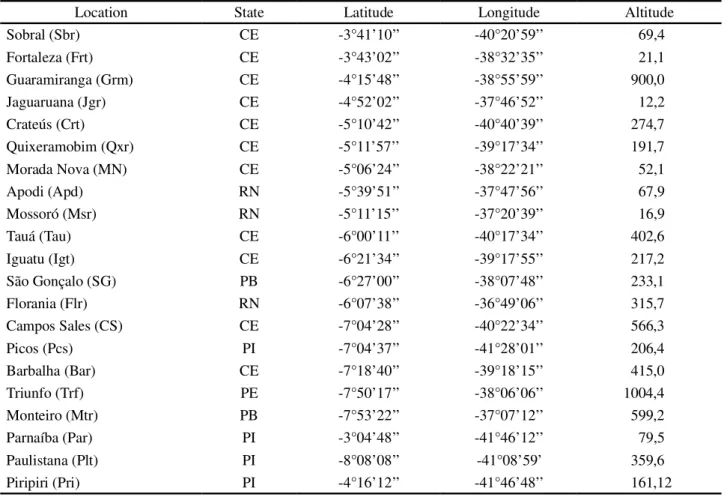
The study was carried out in the state of Ceará, which is located in northeastern Brazil, between the latitudes 2.5º and 8º South, and longitudes 37º and 42º West. According to the Köppen climate classification the study area has three types of climate: BSw’h’, Aw’ and Cw’, with the predominance in approximately 80% of the area of BSw’h’ (hot semiarid). The data used in the study are from the network of meteorological stations in the state (Table 1 and Figure 1), belonging to the National Institute of Meteorology (INMET). The stations from the surrounding states were used to provide boundary conditions.
To estimate the reference evapotranspiration the model proposed by Hargreaves and Samani (1985) was used:
ET
o = 0,0023(Tx - Tn)
0,5(Tm + 17,8)Ra (1)
where: ETo (mm day-1) is the reference evapotranspiration; Tx, Tn and Tm represent the maximum, minimum and average air temperatures respectively (°C); and Ra, the solar radiation at the top of the atmosphere (mm day-1).
For estimates of the spatialised maximum, minimum and average temperatures a multiple linear regression model was tested, with altitude, latitude and longitude as independent variables and the measured temperature as the dependent variable, based on the general quadratic model:
Ti=A0+A1.h+A2.h2+A 3 +A4
2+A 5
+A
6 2+A
7.h.. +A8.h. +A9
(2)
Table 1 - Location of the weather stations
Location State Latitude Longitude Altitude
Sobral (Sbr) CE -3°41’10’’ -40°20’59’’ 69,4
Fortaleza (Frt) CE -3°43’02’’ -38°32’35’’ 21,1
Guaramiranga (Grm) CE -4°15’48’’ -38°55’59’’ 900,0
Jaguaruana (Jgr) CE -4°52’02’’ -37°46’52’’ 12,2
Crateús (Crt) CE -5°10’42’’ -40°40’39’’ 274,7
Quixeramobim (Qxr) CE -5°11’57’’ -39°17’34’’ 191,7
Morada Nova (MN) CE -5°06’24’’ -38°22’21’’ 52,1
Apodi (Apd) RN -5°39’51’’ -37°47’56’’ 67,9
Mossoró (Msr) RN -5°11’15’’ -37°20’39’’ 16,9
Tauá (Tau) CE -6°00’11’’ -40°17’34’’ 402,6
Iguatu (Igt) CE -6°21’34’’ -39°17’55’’ 217,2
São Gonçalo (SG) PB -6°27’00’’ -38°07’48’’ 233,1
Florania (Flr) RN -6°07’38’’ -36°49’06’’ 315,7
Campos Sales (CS) CE -7°04’28’’ -40°22’34’’ 566,3
Picos (Pcs) PI -7°04’37’’ -41°28’01’’ 206,4
Barbalha (Bar) CE -7°18’40’’ -39°18’15’’ 415,0
Triunfo (Trf) PE -7°50’17’’ -38°06’06’’ 1004,4
Monteiro (Mtr) PB -7°53’22’’ -37°07’12’’ 599,2
Parnaíba (Par) PI -3°04’48’’ -41°46’12’’ 79,5
Paulistana (Plt) PI -8°08’08’’ -41°08’59’ 359,6
Piripiri (Pri) PI -4°16’12’’ -41°46’48’’ 161,12
Figure 1 - Spatial distribution of the weather stations
in degrees; h is the altitude in meters; and An are the
regression coefficients.
The generated equations were evaluated by the
coefficient of determination (R2) and F- test at a 5%
level of significance.
The regression coefficients obtained from the
temperature models were applied to specify ETo for the
state of Ceará in the form of thematic maps on a monthly scale, using the Idrisi Andes© software, employing digital maps of longitude, latitude and altitude. For the altitude map, the digital elevation model (DEM) was used, obtained from the SRTM (Shuttle Radar Topography Mission) that resulted from the partnership between NASA (National Aeronautics and Space Administration) and NGA (National Geoespatial-Intelligence Agency), where the aim was to collect radar interferometry data with a view to acquiring detailed topographic models for latitudes between 56ºS and 60ºN.
The whole process of MDE refinement also counted on the help of topographic control data, aimed at validation of the data generated. Radar data were collected during an 11-day mission, and subsequently processed according
to the methodology described by Rabus et al. (2003).
Solar radiation at the top of the atmosphere was
determined using the methodology proposed by Allenet al.
(1998) which considers the 15th day of each month as reference in the calculation of the average ETo for each month.
To compare the results obtained by the Hargreaves and Samani equation (1985) and the temperature maps calculated by the digital terrain model, the ETo was determined by the Hargreaves and Samani method (1985) for each location, based on climate data with the help of the REF-ET software
(ALLEN, 2012). Estimates of ETo by REF-ET software and
those extracted from the generated maps were evaluated using simple error analysis (Equations 3 to 6).
(3)
(4)
(5)
(6)
where: ME is the mean error in mm day -1; SEE is the
standard error of estimation in mm day -1; MPE is the
mean percentage error in %; is the ratio between the
means in %, n is the number of data; yiis the EToHSMaps,
estimated by Hargreaves and Samani (1985) for maps;
xi is the EToHSREF-ET estimated by Hargreaves using
REF-ET; and are the averages of EToHSMaps and
EToHSREF-ET for a given location respectively.
RESULTS AND DISCUSSION
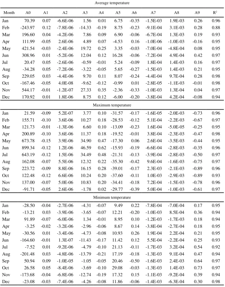
The adjusted coefficients of determination of the regression equations for estimating mean monthly values for the minimum air temperature ranged from 0.98 in December to 0.92 in July; for the mean monthly values for the average air temperature they ranged from 0.98 in September and October, to 0.88 in February; for the mean monthly values for the maximum air temperature they were between 0.98 and 0.93 in April and October respectively (Table 2). It is worth noting that all the regression equations were significant at 5% significance by the F-test.
It was found that the R² values obtained for the minimum as well as for the average and maximum temperatures were similar. This is probably due to the
low variability of temperature data in the months in which they occurred. It was also observed that the maximum monthly value for the coefficient of determination was equal to 0.98, not only for the minimum air temperature, but also for the maximum and average.
The values for R2 for the equations to estimate
the minimum air temperature showed lower values since, of the twelve adjusted equations, six had values of less than 0.95, the same happening with three of the equations for estimating the average air temperature and with one for estimating the maximum. With the equations for estimating the average air temperature it can be seen that the lowest value for the coefficient of
determination (R2 = 0.88) was obtained for the month of
February, indicating lower precision of the estimates.
Pezzopane et al. (2004) studying the spatial
distribution of air temperature in the state of Espírito Santo, obtained values for the adjusted coefficients of determination ranging from 0.88 to 0.94 for the minimum temperature, 0.89 to 0.92 for the average, and 0.94 to 0.98 for the maximum temperature. According to these authors, the fact of the coefficients of determination for the maximum temperature being higher than for the others, may be related to the greater uniformity of this climatic variable in the State.
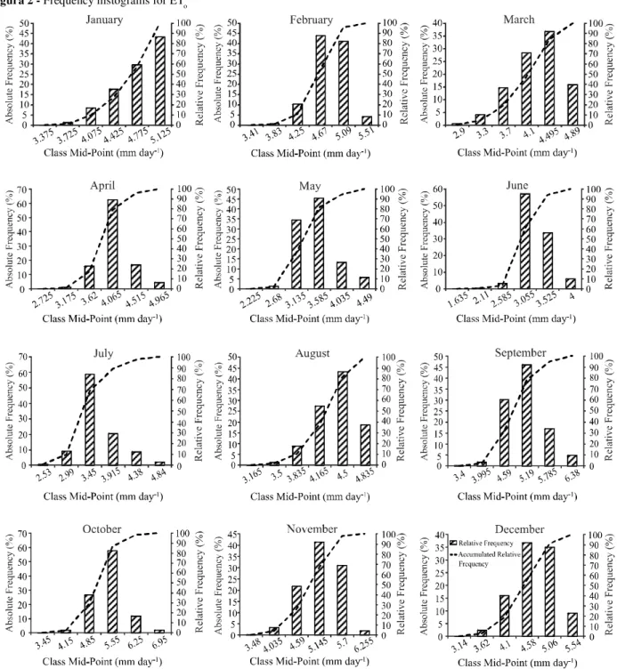
The interval between February and July (Figure 2) presented the lowest demand for evapotranspiration in view of the absolute frequency distribution being offset to the left (lower values); almost all of the annual rainfall and the coldest months in the state being concentrated in this period. Also according to Figure 2, we observe that from August until January the relative frequency values are shifted to the right, i.e. higher values of ETo. October was the month with the highest demand for evapotranspiration in view of the fact that 57.7% of the values are around 5.55 mm day -1. Tabariet al. (2012) in different regions of Iran noted the month of highest demand
with a monthly ETo value of 534.4 mm month-1 was July,
while the lowest value was 25.6 mm month-1 in January.
The inclusion of the digital elevation model in the spatialisation of Tx, Tn and Tmed using GIS, resulted in maps with greater detail and which represent the behavior of this variable as observed in the field and for different states in Brazil (BARDIN, PEDRO JÚNIOR; MORAES, 2010;
MEDEIROSet al., 2005; PEZZOPANEet al., 2004). The
Table 2 - Regression coefficients of the equations for estimating the monthly values for average, maximum and minimum air temperatures with their respective coefficients of determination (R2)
Average temperature
Month A0 A1 A2 A3 A4 A5 A6 A7 A8 A9 R2
Jan 70.39 0.07 -6.6E-06 1.56 0.01 6.75 -0.35 -1.5E-03 1.9E-03 0.26 0.96
Feb -243.97 0.12 -7.8E-06 -14.33 -0.19 8.75 -0.23 -9.1E-04 3.1E-03 0.28 0.88
Mar 196.60 0.04 -4.2E-06 7.86 0.09 6.90 -0.06 -6.7E-04 1.3E-03 0.19 0.93
Apr 111.99 -0.05 2.6E-06 4.89 0.07 -4.53 0.16 -1.0E-06 -1.0E-03 -0.16 0.95
May 421.54 -0.03 -2.4E-06 19.72 0.25 3.35 -0.03 -7.0E-04 -4.8E-04 0.08 0.95
Jun 308.96 0.01 -5.2E-06 12.04 0.12 16.28 -0.06 -7.2E-04 4.9E-04 0.42 0.97
Jul 20.47 0.05 -2.6E-06 -0.59 -0.01 5.24 -0.09 1.8E-04 1.4E-03 0.16 0.97
Aug -34.28 0.05 -7.2E-06 -3.22 -0.05 5.65 -0.27 -1.5E-03 1.4E-03 0.21 0.95
Sep 229.05 0.03 -4.4E-06 9.70 0.11 8.07 -0.24 -4.4E-04 9.7E-04 0.28 0.98
Oct -167.46 -0.05 4.0E-08 -9.62 -0.12 -0.99 0.01 -2.8E-05 -1.1E-03 -0.01 0.98
Nov 544.17 -0.01 -1.2E-07 27.33 0.35 -2.36 -0.33 -1.0E-03 1.3E-04 0.04 0.97
Dec 170.92 0.01 1.8E-06 8.75 0.12 -6.00 -0.20 -3.8E-04 4.2E-04 -0.08 0.94
Maximum temperature
Jan 21.59 -0.09 5.2E-07 3.77 0.10 -31.57 -0.17 -1.6E-05 -2.0E-03 -0.73 0.96
Feb 155.71 -0.10 3.6E-06 10.27 0.18 -28.53 -0.12 5.1E-04 -2.2E-03 -0.67 0.97
Mar 121.73 -0.01 -1.3E-06 6.60 0.10 -13.09 -0.23 1.6E-04 -5.0E-05 -0.25 0.95
Apr 200.89 -0.10 3.6E-06 11.37 0.18 -19.52 -0.01 3.8E-04 -2.3E-03 -0.47 0.98
May 673.78 -0.15 3.9E-06 34.90 0.47 -17.30 0.06 2.6E-04 -3.5E-03 -0.44 0.95
Jun 899.34 -0.12 1.2E-06 46.59 0.62 -15.93 -0.19 -6.6E-04 -2.8E-03 -0.35 0.96
Jul 643.19 -0.12 1.5E-06 34.49 0.48 -21.31 -0.13 -3.9E-04 -2.8E-03 -0.50 0.97
Aug 162.08 -0.07 5.5E-06 12.32 0.22 -35.30 -0.42 9.6E-04 -1.6E-03 -0.75 0.97
Sep 223.72 -0.09 8.8E-06 16.15 0.28 -39.01 -0.17 2.3E-03 -2.1E-03 -0.89 0.96
Oct 122.48 -0.12 6.6E-06 10.24 0.20 -37.60 -0.11 1.0E-03 -2.9E-03 -0.89 0.93
Nov 137.00 -0.07 5.0E-06 10.83 0.20 -34.41 -0.18 7.2E-04 -1.5E-03 -0.78 0.96
Dec -91.71 -0.05 2.6E-06 -1.78 0.02 -29.77 -0.39 5.0E-04 -1.0E-03 -0.61 0.97
Minimum temperature
Jan -28.50 -0.04 -2.7E-06 -4.31 -0.07 9.49 0.22 -7.8E-04 -7.0E-04 0.17 0.95
Feb -13.21 0.03 -3.9E-06 -3.65 -0.07 12.21 -0.20 -1.0E-03 8.5E-04 0.36 0.94
Mar 91.89 -0.07 -6.0E-06 1.34 -0.01 8.95 0.10 -1.2E-03 -1.7E-03 0.18 0.94
Apr -3.25 -0.02 -3.2E-06 -2.96 -0.06 8.67 0.14 -3.8E-04 -2.7E-04 0.18 0.95
May -30.56 0.01 -3.4E-06 -4.73 -0.08 10.93 0.26 1.9E-04 2.2E-04 0.21 0.95
Jun -164.60 -0.01 1.3E-07 -11.43 -0.17 11.42 0.12 5.5E-04 -2.2E-04 0.25 0.93
Jul -7.52 0.01 -9.2E-06 -4.79 -0.10 21.13 -0.11 -1.7E-03 3.2E-04 0.54 0.92
Aug -201.48 0.03 -4.8E-06 -13.79 -0.21 17.19 -0.18 -1.3E-03 9.1E-04 0.47 0.94
Sep 50.94 0.09 -1.0E-05 -1.05 -0.05 20.46 -0.50 -1.6E-03 2.4E-03 0.64 0.97
Oct 26.58 0.05 -8.4E-06 -3.69 -0.10 29.08 -0.03 -1.3E-03 1.4E-03 0.73 0.97
Nov -173.68 -0.04 -6.8E-06 -12.74 -0.19 17.32 0.15 -1.1E-03 -9.2E-04 0.39 0.94
Figura 2 - Frequency histograms for ETo
to run the equations on similarly detailed topographic maps
Combining maps of the spatial distribution of ETo with
the spatial distribution of the meteorological variables will provide an important basis for the study of hydrological and
climate modelling (AHMADet al., 2005; FOOLADMAND;
HAGHIGHAT, 2007; KONGOet al., 2011).
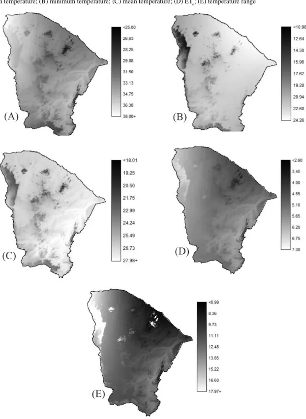
The thematic map of maximum air temperature (Figure 3A) showed values varying from 25 °C to 38 °C. It was also found that for almost all regions of the state of
in the regions of mountains and plateaus that cross the states of Ceará and Piauí, such as Serra Grande, the Chapada do Araripe and Serra Dois Irmãos. However,
Figure 3 - Maps of temperature and reference evapotranspiration in the month of maximum demand, for the state of Ceará: (A) maximum temperature; (B) minimum temperature; (C) mean temperature; (D) ETo; (E) temperature range
The spatial modeling of ETo gives an understanding of the spatial and temporal variability of the demand for water in different regions of the state (Figure 3D). Xuet al.
(2006) state that spatial distribution maps provide valuable information for the planning and management of water resources in a basin or region, since the spatial distribution
of the seasonal and annual values for ETo is an important
component of the hydrological cycle. From Figure 3D it can clearly be seen that the areas with a lower value for ETo in the peak month are in the region of Serra de Guaramiranga, while the smallest values of ETo were observed in the region of the Chapada da Ibiapaba (Serra Grande), going against the more
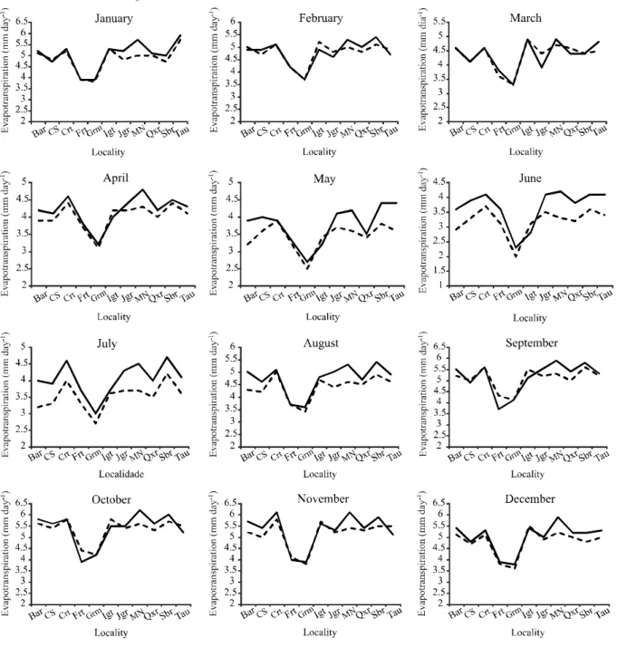
Figure 4 - Trend analysis of ETo obtained from the map and observed at the stations
Figure 4 shows the comparison between the ETo obtained from the temperature maps for the pixel containing a station, and the values obtained from the climatic data at that station. Comparison of the results between the methods tested, clearly shows variability from one location to another. It can be seen that for the stations of Morada Nova, Quixeramobim and Sobral the values obtained by the proposed method were always lower than those obtained by REF-ET, except in March. While the stations in Fortaleza and Iguatu presented the best results throughout the year, with closer values between methodologies.
It is worth noting that the Hargreaves and Samani equation (1985) tends to overestimate ETo in humid regions and underestimate it in very dry regions and in those regions with higher wind speeds (TEMESGEN; ALLEN; JENSEN, 1999; XU; SINGH, 2002). Therefore, the Hargreaves and Samani equation (1985) requires local calibration before
being applied to estimate ETo in any particular region
(BAUTISTA, BAUTISTA, 2009; GAVILANet al., 2006;
FOOLADMAND; HAGHIGHAT, 2007).
Analyzing the values of , It can be seen that in four
months only, the values of ETo were underestimated when
obtained from the temperature map in relation to the ETo
obtained by REF-ET (Table 3). The proposed methodology
for estimating ETo by the Hargreaves and Samani equation
(1985) from altitude data produced satisfactory estimates, considering that seven months showed values that had been under or overestimated by less than 5% ( ).
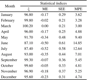
Table 3 - Ratio of the mean ( ), mean error (ME), standard error of estimation (SEE) and mean percentage error (MPE) between ETo estimated with the digital elevation model (EToHSMaps), and the REF-ET software (EToHSREF-ET) as estimated by Hargreaves and Samani (1985)
Taking into consideration only the average of all the locations for each month, the values of ME ranged
from 0.0 to -0.52 mm d-1, with a mean of -0.22 mm d-1
(Table 3). SEE values ranged from 0.21 to 0.61 mm d-1
with a mean value of 0.31 mm d-1. Ratios between the
mean values ( ) obtained with the two methods, showed that the greatest underestimation observed was 12.9% (June). Considering only the months of June and July,
when the ETo values obtained from the map showed
the greatest underestimates, the values obtained for the mean percentage error (MPE) were 14.85 and 12.64% for the months of June and July respectively.
CONCLUSIONS
1. The proposed methodology did not show good results in the coldest months of the year (June and July) in the state of Ceará;
2. The methodology proposed for spatialising ETo by
means of the Hargreaves and Samani equation (1985) using temperature maps obtained by the SRTM digital elevation model, proved to be a viable alternative in view of the results of the statistical analysis when compared to the standard method.
REFERENCES
AHMAD et al. A new technique to estimate net groundwater use across large irrigated areas by combining remote sensing and water balance approaches, Rechna Doab, Pakistan. Hydrogeology Journal, v. 13, n. 5/6, p. 653-664, 2005. ALLEN, R. G. A Penman for all seasons. Journal Irrigation Drainage Engineering, v. 112, n. 4, p. 348-368, 1986. ALLEN, R. G.et al.Crop evapotranspiration: guidelines for computing crop water requirements. Rome: FAO, 1998. (FAO Irrigation and Drainage Paper, 56).
ALLEN, R. G. REF-ET: Reference Evapotranspiration Calculation Software for FAO and ASCE Standardized Equations. University of Idaho, 2012.
BARBOSA, F. C.; TEIXEIRA, A. dos S.; GONDIM, R. S. Espacialização da evapotranspiração de referência e precipitação efetiva para estimativa das necessidades de irrigação na região do Baixo Jaguaribe - CE.Revista Ciência Agronômica, v. 36, n. 1, p. 24-33, 2005.
BARDIN, L.; PEDRO JÚNIOR, M. J.; MORAIS, J. F. L. Estimativa das Temperaturas máximas e mínimas do ar para a região do Circuito das Frutas, SP. Revista Brasileira de Engenharia Agrícola e Ambiental, v. 14, n. 6, p. 618-624, 2010.
Month Statistical índices
ME SEE MPE
January 96.80 -0.17 0.29 3.62
February 99.80 -0.02 0.21 3.28
March 100.20 0.00 0.21 3.00
April 96.00 -0.17 0.25 4.88
May 91.70 -0.34 0.48 9.40
June 87.10 -0.50 0.61 14.85
July 87.40 -0.52 0.58 12.64
August 93.00 -0.35 0.44 7.01
September 99.30 -0.07 0.36 5.45
October 99.60 -0.05 0.33 4.81
November 96.90 -0.18 0.37 5.25
BAUTISTA, F.; BAUTISTA, D. Calibration of the equations of Hargreaves and Thornthwaite to estimate the potential evapotranspiration in semi-arid and subhumid tropical climates for regional applications.Atmósfera, v. 22, n. 4, p. 331-348, 2009. CARGNELUTTI FILHO, A.; MALUF, J. R. T.; MATZENAUER, R. Coordenadas geográficas na estimativa das temperaturas máximas e médias decendiais do ar no Estado do Rio Grande do Sul.Ciência Rural, v. 38, n. 9, p. 2448-2456, 2008.
DROOGERS, P.;ALLEN, R. G. Estimating reference evapotranspiration under inaccurate data conditions.Irrigation Drainage System,v. 16, n. 1, p. 33-45, 2002.
FOOLADMAND, H. R.; HAGHIGHAT, M. Spatial and temporal calibration of Hargreaves equation for calculating monthly ETO based on Penman-Monteith method.Irrigation and Drainage, v. 56, n. 4, p. 439-449, 2007.
GAVILÁN, P. et al. Regional calibration of Hargreaves equation for estimating reference ET in a semiarid environment.Agricultural Water Management,v. 81, n. 3, p. 257-281, 2006.
GAVILÁN, P.; BERENGENA, J.; ALLEN, R. G. Measuring versus estimating net radiation and soil heat flux: impact on Penman-Monteith reference ET estimates in semiarid regions. Agricultural Water Management,v. 89, n. 3, p. 275-286, 2007. HARGREAVES, G. H.; SAMANI, Z. A. Reference crop evapotranspiration from temperature. Applied Engineered Agricultural, v. 1, n. 2, p. 96-99, 1985.
KONGO, M. V. et al. Evaporative water use of different land uses in the upper-Thukela river basin assessed from satellite imagery.Agricultural Water Management, v. 98, n. 11, p. 1727-1739, 2011.
LOPEZ-URREA, R. et al. An evaluation of two hourly reference evapotranspiration equations for semiarid conditions. Agricultural Water Management, v. 86, n. 3, p. 277-282, 2006.
MEDEIROS, S. de S. et al. Estimativa e espacialização das temperaturas do ar mínimas, médias e máximas na Região
Nordeste do Brasil.Revista Brasileira de Engenharia Agrícola e Ambiental, v. 9, n. 2, p. 247-255, 2005.
PEREIRA, A. R.; PRUITT, W. O. Adaptation of the Thornthwaite scheme for estimating daily reference evapotranspiration. Agricultural Water Management,v. 66, n. 3, p. 251–257, 2004. PEZZOPANE, J. E. M. et al. Espacialização da temperatura do ar no Estado do Espírito Santo. Revista Brasileira de Agrometeorologia, v. 12, n. 1, p. 151-158, 2004.
RABUS, B.et al. The Shuttle Radar Topography Mission - a new class of digital elevation models acquired by spaceborne radar. ISPRS. Journal of Photogrammetry & Remote Sensing, v. 57, n. 4, p. 241-262, 2003.
ROCHA, É. J. T.et al. Estimativa da Eto pelo modelo Penman-Monteith FAO com dados mínimos integrada a um Sistema de Informação Geográfica.Revista Ciência Agronômica, v. 42, n. 1, p. 75-83, 2011.
TABARI, H.et al. Spatial distribution and temporal variation of reference evapotranspiration in arid and semi-arid regions of Iran.Hydrological Processes, v. 26, n. 4, p. 500-512, 2012. TEMESGEN, B.; ALLEN, R. G.; JENSEN, D. T. Adjusting temperature parameters to reflect well-water conditions.Journal of Irrigation and Drainage Engineering, v. 125, n. 1, p. 26-33, 1999. VENTURA, F.et al. An evaluation of common evapotranspiration equations.Irrigation Science, v. 18, n. 4, p. 163-170, 1999. WALTER, I. A. et al. ASCE’s standardized reference evapotranspiration equation.Proc. 4th National Irrigation Symp. American Society of Agricultural Engineers, p. 209-215. 2000. XU C.Y.; SINGH, V. P. Cross comparison of empirical equations for calculating potential evapotranspiration with data from Switzerland.Water Research Management, v. 16, p. 197-219, 2002.