Creating long term gridded fields of reference evapotranspiration in Alpine terrain based on a re-calibrated Hargreaves method

(1)

HESSD

12, 5055–5082, 2015

Creating long term gridded fields of

reference evapotranspiration

K. Haslinger and A. Bartsch

Title Page

Abstract Introduction

Conclusions References

Tables Figures

◭ ◮

Back Close

Full Screen / Esc

Printer-friendly Version Interactive Discussion

Discussion

P

a

per

|

Discussion

P

a

per

|

Discussion

P

a

per

|

Discussion

P

a

per

|

Hydrol. Earth Syst. Sci. Discuss., 12, 5055–5082, 2015 www.hydrol-earth-syst-sci-discuss.net/12/5055/2015/ doi:10.5194/hessd-12-5055-2015

This discussion paper is/has been under review for the journal Hydrology and Earth System Sciences (HESS). Please refer to the corresponding final paper in HESS if available.

Creating long term gridded fields of

reference evapotranspiration in Alpine

terrain based on a re-calibrated

Hargreaves method

K. Haslinger and A. Bartsch

Central Institute for Meteorology and Geodynamics (ZAMG), Climate Research Department, Vienna, Austria

Received: 7 April 2015 – Accepted: 9 May 2015 – Published: 28 May 2015

Correspondence to: K. Haslinger (klaus.haslinger@zamg.ac.at)

(2)

HESSD

12, 5055–5082, 2015

Title Page

Tables Figures

◭ ◮

Back Close

Full Screen / Esc

Discussion

P

a

per

|

Discussion

P

a

per

|

Discussion

P

a

per

|

Discussion

P

a

per

|

Abstract

A new approach for the construction of high resolution gridded fields of reference evap-otranspiration for the Austrian domain on a daily time step is presented. Forcing fields of gridded data of minimum and maximum temperatures are used to estimate reference evapotranspiration based on the formulation of Hargreaves. The calibration constant in 5

the Hargreaves equation is recalibrated to the Penman–Monteith equation, which is recommended by the FAO, in a monthly and station-wise assessment. This ensures on one hand eliminated biases of the Hargreaves approach compared to the formulation of Penman–Monteith and on the other hand also reduced root mean square errors and relative errors on a daily time scale. The resulting new calibration parameters are in-10

terpolated in time to a daily temporal resolution for a standard year of 365 days. The overall novelty of the approach is the conduction of surface elevation as a predictor to estimate the re-calibrated Hargreaves parameter in space. A third order spline is fitted to the re-calibrated parameters against elevation at every station and yields the statistical model for assessing these new parameters in space by using the underlying 15

digital elevation model of the temperature fields. Having newly calibrated parameters for every day of year and every grid point, the Hargreaves method is applied to the tem-perature fields, yielding reference evapotranspiration for the entire grid and time period from 1961–2013. With this approach it is possible to generate high resolution reference evapotranspiration fields starting when only temperature observations are available but 20

re-calibrated to meet the requirements of the recommendations defined by the FAO.

1 Introduction

The water balance in its most general form is determined by the fluxes of precipitation, change in storage and evapotranspiration (Shelton, 2009). Particularly for the latter, measurement is rather costly, since it requires sophisticated techniques like eddy cor-25

(3)

evapo-HESSD

12, 5055–5082, 2015

Title Page

Tables Figures

◭ ◮

Back Close

Full Screen / Esc

Discussion

P

a

per

|

Discussion

P

a

per

|

Discussion

P

a

per

|

Discussion

P

a

per

|

transpiration as part of the water balance equation is mostly assessed from the poten-tial evapotranspiration (PET). PET refers to the maximum moisture loss from the sur-face, determined by meteorological conditions and the surface type, assuming unlim-ited moisture supply (Lhomme, 1997). Since surface conditions determine the amount of PET, the concept of reference evapotranspiration (ET0) was introduced (Doorenbos 5

and Pruitt, 1977). ET0 refers to the evapotranspiration from a standardized vegetated surface (grass) under unrestricted water supply, making ET0 independent of soil prop-erties. Numerous methods exist for estimating ET0; differences arise in the complexity and the amount of necessary input data for calculation.

A standard method, also recommended by the FAO (Allen et al., 1998), is the 10

Penman–Monteith (PM) formulation of ET0. This equation is considered the most re-liable estimate and serves as a standard for comparisons with other methods (Allen et al., 1998). PM is fully physically based and requires four meteorological parameters (air temperature, wind speed, relative humidity and net radiation). It utilizes energy bal-ance calculations at the surface to derive ET0 and is therefore considered a radiation 15

based method (Xu and Singh, 2000).

On the contrary, much simpler methods which use air temperature as a proxy for ra-diation (Xu and Singh, 2001) have been developed to overcome the shortcoming of PM of not having sufficient input data. In this paper, the method of Hargreaves (HM, Har-greaves et al., 1985) is used. It requires minimum and maximum air temperature and 20

extraterrestrial radiation, which can be derived by the geographical location and the day of year. Though much easier to calculate as temperature observations are dense and easily accessible, one has to be aware that the HM, among most temperature based estimates, are developed for distinct studies and/or regions, representing a rather dis-tinct climatic setting (Xu and Singh, 2001). To avoid large errors, these methods need 25

(4)

HESSD

12, 5055–5082, 2015

Title Page

Tables Figures

◭ ◮

Back Close

Full Screen / Esc

Discussion

P

a

per

|

Discussion

P

a

per

|

Discussion

P

a

per

|

Discussion

P

a

per

|

In this paper the method for constructing a dataset of ET0 on a daily time resolution and a 1 km spatial resolution based on the method of Hargreaves is presented. The HM is calibrated to the PM as the standard for estimating ET0 on a station-wise assess-ment. Numerous studies describe re-calibration procedures for the HM (Bautista et al., 2009; Pandey et al., 2014; Gavilán et al., 2006) in order to achieve similar results to 5

the PM, which serves as a reference. There are also some studies describing methods for creating interpolated ET0 estimates (e. g. Aguila and Polo, 2011; Todorovic et al., 2013). However, two main methodological frameworks emerged for the interpolation of ET0 (McVicar et al., 2007): (i) interpolation of the forcing data and then calculating ET0, or (ii) calculating ET0 at every weather station and the interpolating ET0 onto the 10

grid. In this paper we follow the first approach. Spatially interpolated daily temperature measurements (minimum and maximum temperature) are used as forcing fields for the application of the Hargreaves formulation of ET0. The novelty of this study is the appli-cation of elevation as a predictor for the interpolation of the re-calibrated HM calibration parameter. Furthermore, these new calibration parameters are also variable in time, by 15

changing day-by-day for all days of the year. This approach goes a step further than the method of Aguilar and Polo (2011) which derived one new calibration parameter for the dry and one for the wet season of the year.

The presented dataset aims to use the best of two worlds by (i) using a method for estimating ET0 that is calibrated to the standard algorithm as defined by the FAO 20

and (ii) being applicable to a comprehensive, long-term forcing dataset and on a high temporal and spatial resolution.

2 Forcing data

The foundation of the ET0 calculations are high resolution gridded dataset of daily min-imum and maxmin-imum temperatures calculated for the Austrian domain (SPARTACUS, 25

(5)

HESSD

12, 5055–5082, 2015

Title Page

Tables Figures

◭ ◮

Back Close

Full Screen / Esc

Discussion

P

a

per

|

Discussion

P

a

per

|

Discussion

P

a

per

|

Discussion

P

a

per

|

dataset starting in 1961 and reaching down to the present day. For the conduction of the ET0 fields, the SPARTACUS temperature forcing is used for the period 1961–2013. The interpolation algorithm is tailored for complex, mountainous terrain with spatially complex temperature distributions. SPARTACUS also aims to ensure temporal consis-tency through a fixed station network over the whole time period, providing robust trend 5

estimations in space. As for the SPARTACUS dataset the SRTM (Shuttle Radar Topog-raphy Mission, Farr and Kobrick, 2000) version 2 Digital Elevation Model (DEM) is used in this study.

SPARTACUS provides the input data for calculating ET0 following the Hargreaves method (HM, Hargreaves and Samani, 1982; Hargreaves and Allen, 2003). However, 10

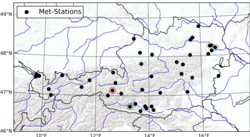
a recalibration of the HM is necessary to avoid considerable estimation errors. This is carried out in a station wise assessment. Data of 42 meteorological stations (provided by the Austrian Weather Service ZAMG) is used to monthly calibrate the HM to the Penman–Monteith Method (PM). Figure 1 shows the location of the stations, which are spread homogeneously among the Austrian domain and also comprise rather different 15

elevations and environmental settings (Table 1). Data of daily global radiation, wind speed, humidity, maximum and minimum temperatures covering the period 2004–2013 are used to calculate ET0 simultaneously with HM and PM.

3 Methods

3.1 Estimating reference evapotranspiration

20

Numerous methods exist for the estimation of ET0, which is defined as the maximum moisture loss from the land surface limited only by energy endowment (Shelton, 2009). They can roughly be classified as temperature based and radiation based estimates (Xu and Singh, 2000, 2001; Bormann, 2011). Following the recommendations of the FAO (Allen et al., 1998) the radiation-based Penman–Monteith Method (PM) provides 25

(6)

over-HESSD

12, 5055–5082, 2015

Title Page

Tables Figures

◭ ◮

Back Close

Full Screen / Esc

Discussion

P

a

per

|

Discussion

P

a

per

|

Discussion

P

a

per

|

Discussion

P

a

per

|

all shortcoming of the PM is the data intense calculation algorithm which requires daily values of global radiation, wind speed, humidity, maximum and minimum temperatures. Data coverage for these variables is usually rather sparse particularly if gridded data is required. ET0 following the PM is calculated as displayed in Eq. (1):

E=0.408∆(RN−G)+γ

900

T+273u2(es−ea)

∆ +γ(1₊0.34u2)

(1) 5

whereE is the reference evapotranspiration [mm day−1_],_R

N is the net radiation at the crop surface [MJ m−2_day−1_], _G _{is the soil heat flux density [MJ m}−2_day−1_], _T _{is the}

mean air temperature at 2 m height [◦_C],_u

2is the wind speed at 2 m height [m s− 1

],es is the saturation vapour pressure [kPa],ea is the actual vapour pressure [kPa]; giving the vapour pressure deficit by subtracting ea from es; ∆ is the slope of the vapour 10

pressure curve [kPa◦_C−1_{] and} _γ _{is the psychrometric constant [kPa}◦_C−1_{]. Given the}

time resolution of one day the soil heat flux term is set to zero. The calculation of the other individual terms of Eq. (1) is described in Allen et al. (1998).

In contrast to the radiation based PM, the HM is based on daily minimum and max-imum temperatures (Tmin, Tmax). Hargreaves (1975) stated from regression analysis 15

between meteorological variables and measured ET0 that temperature multiplied by surface global radiation is able to explain 94 % of the variance of ET0 for a five day period (see Hargreaves and Allen, 2003). Furthermore, wind and relative humidity ex-plained only 10 and 9 % respectively. Additional investigations by Hargreaves led to an assessment of surface radiation which can be explained by extra-terrestrial radiation 20

at the top of the atmosphere and the diurnal temperature range as an indicator for the percentage of possible sunshine hours. The final form of the Hargreaves equation is given by:

E=C(Tmean+17.78)(Tmax−Tmin)0.5Ra (2)

where E is the reference evapotranspiration [mm day−1_], _T

mean, Tmax and Tmin are 25

the daily mean, maximum and minimum air temperatures [◦_{C] respectively and} _R

(7)

HESSD

12, 5055–5082, 2015

Title Page

Tables Figures

◭ ◮

Back Close

Full Screen / Esc

Discussion

P

a

per

|

Discussion

P

a

per

|

Discussion

P

a

per

|

Discussion

P

a

per

|

is the water equivalent of the extra-terrestrial radiation at the top of the atmosphere [mm day−1

]. C is the calibration parameter of the HM and was set to 0.0023 in the original Hargreaves et al. (1985) publication.

Following these formulations the ET0 for all stations was calculated for the period 2004–2013. As PM is declared by the FAO as the preferred ET0 estimation model, it 5

serves as the reference for the following comparison between both methods. Figure 2a shows, as an example, the daily time series of ET0 as derived by PM (ET0_p) and HM (ET0_h) in the year 2004 at the station Wien_Hohewarte. The differences between those two are obvious as ET0_p shows clearly higher variability, with ET0_h underesti-mating the upward peaks in the cold season and downward peaks in the warm season. 10

This feature is more noticeably in Fig. 2b, which shows the monthly averages over all stations, indicating the spread among all 42 stations. Here, an underestimation of the ET0_h compared to ET0_p from October to April is counteracted by an overestimation between May and September. On the other hand, ET0_h shows higher spread among stations compared to ET0_p except for November to January.

15

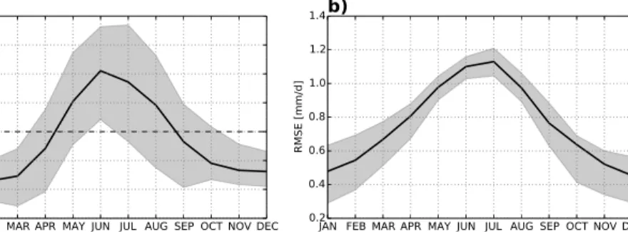
These features are also reflected in the bias of ET0_h compared to ET0_p as can be seen in Fig. 3a. The average monthly bias over all stations is negative in the cold season with largest deviations in February of 0.3 mm day−1_{, compared to the peak}

average positive bias in June of 0.4 mm day−1_{. The annual cycle of the Root Mean}

Squared Error (RMSE) of ET0_h as displayed in Fig. 3b shows peak values in summer 20

mainly due to the higher absolute values in the warm season compared to wintertime. The RMSE in December is around 0.5 mm day−1 _{compared to 1.1 mm day}−1 _{in July,}

showing some more spread in wintertime compared to summer.

3.2 Calibration

In order to achieve a meaningful representation of ET0 by HM, an adjustment of the 25

(8)

equa-HESSD

12, 5055–5082, 2015

Title Page

Tables Figures

◭ ◮

Back Close

Full Screen / Esc

Discussion

P

a

per

|

Discussion

P

a

per

|

Discussion

P

a

per

|

Discussion

P

a

per

|

tion, as also proposed by Bautista et al. (2009):

Cadj=0.0023/(EH/EP) (3)

whereCadj represents the new calibration parameter of the HM,EHis the original ET0 from HM, using a C of 0.0023 andEP is the ET0 from PM. As a result, a new set ofC values for every month and every station is available.

5

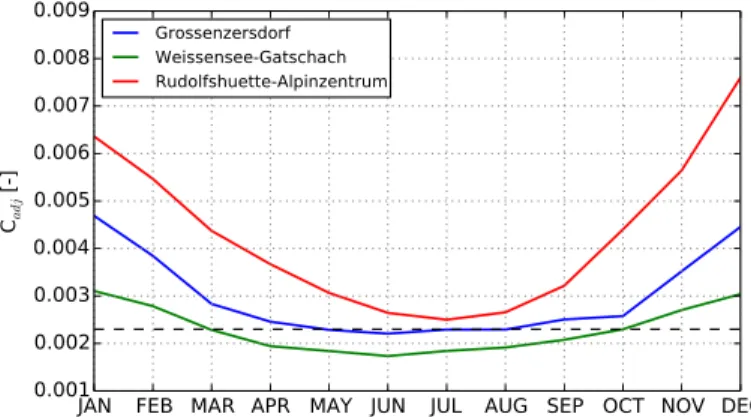
Figure 4 shows the adjustedCvalues for three exemplary stations. Cadj is generally higher in winter and autumn compared to the original value indicated by the dashed line at 0.0023. It is also obvious that at station Grossenzersdorf the original value is matching rather well to the Cadj from April to October, in the other months the ad-justed values are clearly higher. On the contrary, at station Weissensee_Gatschach 10

Cadjis lower than 0.0023 except for the months from November to February. At station Rudolfshuette-Alpinzentrum the adjusted values are above the original ones all time of the year, reaching rather high values in wintertime of about 0.007. These results clearly underpin the necessity for a re-calibration ofC in order to receive sound ET0 from temperature.

15

After determining the values forCadj the ET0 was re-calculated with these new cal-ibration parameter values (ET0_h.c). For sakes of simplicity for this first assessment the monthly values ofCadj where used for all days of the month respectively, no tem-poral interpolation was conducted. As a result, the monthly mean bias, as was shown in Fig. 4a, is reduced to zero at every station. Furthermore, the RMSE has also slightly 20

decreased by 0.1 to 0.2 mm day−1

, as can be seen in Fig. 5a. The Relative Error (RE) has also decreased, from around 50 % to fewer than 40 % in January for example (cf. Figure 5b). The improvements regarding RE in summer are lower due to the higher absolute values of ET0 in the warm season.

The complete monthly mean time series from 2004 to 2013 of ET0_p, ET0_h and 25

(9)

sta-HESSD

12, 5055–5082, 2015

Title Page

Tables Figures

◭ ◮

Back Close

Full Screen / Esc

Discussion

P

a

per

|

Discussion

P

a

per

|

Discussion

P

a

per

|

Discussion

P

a

per

|

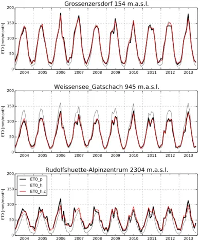
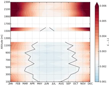
tion Weissensee-Gatschach is considerably reduced with ET0_h.c. These features in combination with the information on the altitude of the given stations provide some in-formation on more general characteristics ofCadj and the effects of the calibration. It seems that there is an altitude-dependence ofCadj, which is displayed in more detail in Fig. 7. It shows the monthly averageCadjfor stations which where binned to distinct 5

classes of altitude ranging from 100 to 2300 m in steps of 100 m. As already seen in Fig. 4 as an example for three stations, C_adj is clearly higher in winter than the un-adjusted value. From April to September Cadj is lower than 0.0023 up to altitudes of 1500 m.a.s.l., lowest values are visible in May to August between altitudes of 400 to 1000 m.a.s.l.

10

3.3 Temporal and spatial interpolation of the Hargreaves calibration parameter

C_adj

The monthly adjusted calibration parameters are now interpolated in space and time in order to receive a congruent overlay ofC_adjover the SPARTACUS grid for every day of year. As a first step, the monthlyCadjvalues at every station are linearly interpolated 15

to daily values to avoid stepwise changes and therefore abrupt shifts ofCadj between months. This is carried out for a standard year with length of 365 days. The result is a time series of daily changing values of Cadj over the course of the year, available for every station, stretching over different altitudes and therefore yielding 42 different annual time series ofCadj.

20

Subsequently the daily, station-wise values ofCadjare interpolated in space. As was shown in the previous section,Cadjchanges with altitude. Figure 8 shows the adjusted calibration parameters plotted against altitude for the monthly means ofCadj. From this Figure it comes clear that this relationship is not linear. Cadj is decreasing from the very low situated stations until altitudes between 500 and 1000 m.a.s.l. Going further 25

(10)

com-HESSD

12, 5055–5082, 2015

Title Page

Tables Figures

◭ ◮

Back Close

Full Screen / Esc

Discussion

P

a

per

|

Discussion

P

a

per

|

Discussion

P

a

per

|

Discussion

P

a

per

|

pared to the cluster of stations between 2000 and 2400 m.a.sl. This feature indicates that the relationship above 1000 m.a.s.l. might not be linear. Taking all this characteris-tics into account, a higher order polynomial fit was chosen to describe theCadj-altitude relation. As shown in Fig. 8 a third order polynomial fit, indicated by the red line, is applied. Using the underlying DEM of the SPARTACUS dataset it is possible to deter-5

mine adjusted calibration parameters for every grid point in space by this relationship. This procedure is applied for every day of the daily interpolated station-wiseC_adj. The result is a gridded dataset ofCadj for the SPARTACUS domain for 365 time steps from 1 January to 31 December. Figure 9 shows two examples ofCadj distribution in space on 1 January (a) and 1 July (b). Particularly in January the altitude dependence of the 10

calibration parameter is clearly standing out, showing rather high values ofCadj at the main Alpine crest. In contrast to winter the spatial variations in summer are smaller, only some central Alpine areas between 1000 and 3000 m.a.s.l. are appearing in somewhat di_fferent shading than the surrounding low lands.

Having these griddedCadj values the ET0_h.c is calculated for every grid point and 15

day since 1961 to 2013. In the case of leap years theCadj grid of 28 February is also used for 29 February.

4 Results

Figure 10a shows the climatological mean (1961–2013) of the annual sum of ET0 over the whole domain. Altitude as a main control on surface temperature, and there-20

fore consequently on ET0, clearly stands out. Lowest mean daily values of around 1.4 mm day−1 _{are apparent on the highest mountain ridges of the main Alpine crest.}

Highest values of up to 2.4 mm day−1 _{are found on the inner Alpine valley floors and}

the eastern and southern low lands. Interestingly, the northern and eastern low lands show lower ET0 values than the southern basins and valleys. This feature might result 25

(11)

HESSD

12, 5055–5082, 2015

Title Page

Tables Figures

◭ ◮

Back Close

Full Screen / Esc

Discussion

P

a

per

|

Discussion

P

a

per

|

Discussion

P

a

per

|

Discussion

P

a

per

|

conditions. Bigger diurnal temperature ranges also increase ET0 in the HM, since it as a proxy for radiation.

Figure 10b shows exemplary the ET0 field of 8 August 2013. On that particular day, temperatures reached for the first time in the instrumental period above 40◦_{C in Austria}

at some stations in the East and South. Values of ET0 are particularly high, reaching up 5

to 7 mm day−1

in some areas in the Southeast. That day was also characterized by an approaching cold front, bringing rain, dropping temperatures and overcast conditions from the West. This is featured as well in the ET0 field, showing a considerable gradient from West to East, with nearly zero ET0 at the headwaters of the Inn River in the far Southwest of the domain. Furthermore, the implications of overcast conditions in the 10

West with lower altitudinal gradients of ET0 compared to the East with sunny conditions and distinct gradients along elevation are visible.

July, the month with the highest absolute values of ET0 shows considerable varia-tions in the last 53 years. As an example, the mean anomaly of ET0 in July of 1983 with respect to the July mean of 1961–2013 is displayed in Fig. 11a. This month was char-15

acterized by a considerable heat wave and mean temperature anomalies of +3.5◦_C

which also affected ET0. The absolute anomaly of ET0 reaches above 1 mm day−1

with respect to the climatological mean in some areas. The relative anomaly is in a range between 10 to 30 % (Fig. 11c). On the other hand, July of 1979 was rather cool with temperatures 1.5◦_{C below the climatological mean and accompanied by}

20

a strong negative anomaly in sunshine duration, particularly in the areas north of the main Alpine crest. The features implicated a distinctly negative anomaly of ET0 in this particular month (Fig. 11b). The absolute anomaly stretches between 0 and more than

−1 mm day−1, equivalent to a relative anomaly of 0 to−30 % (Fig. 11d). The negative

signal is stronger in the areas north of the Alpine crest, zero anomalies are found in 25

the some areas south of the main Alpine crest.

(12)

formula-HESSD

12, 5055–5082, 2015

Title Page

Tables Figures

◭ ◮

Back Close

Full Screen / Esc

Discussion

P

a

per

|

Discussion

P

a

per

|

Discussion

P

a

per

|

Discussion

P

a

per

|

tion without calibration (12b) and with re-calibration as described in this study (12a). Overall, the gradient along elevation of ET0 is larger in the non-calibrated field. Partic-ularly in this time of the year with large absolute values, the re-calibration has a consid-erable impact, althoughCadjin August is relatively small compared to winter. However, ET0_h.c is clearly higher above 1500 m.a.s.l. The bias shows a distinct spatial pat-5

tern with altitude as the driving mechanism. In the Alpine areas the underestimation of ET0_h is up to 1 mm day−1 _{or 30 %. On the other hand, ET0_h shows an}

overes-timation in the lowlands, but the bias in these areas is smaller, around 0.5 mm d−1

or 15 %.

5 Discussion

10

By comparing the characteristics of ET0 based on HM and PM on a daily time step it came clear that a re-calibration ofCwithin the formulation of Hargreaves follows distinct patterns. The values of Cadj show markedly variations in space and time (over the course of the year). It turned out, that a monthly re-calibration ofCreveals an annual cycle ofCadj, withCadj being close to the original value of 0.0023 in the warm season 15

(April–October) and low elevations. Going to higher elevations unfolded decreasingC_adj in the warm season until roughly 1000 m.a.s.l. Reaching altitudes above 1700 m.a.s.l., Cadjis generally above the original 0.0023, particularly in the cold season (November– March). This altitude dependency of the calibration parameter in HM is mentioned in Samani (2000), but was relativized by this relationship being affected by latitude. Aguila 20

and Polo (2011) also found that the original HM using a C of 0.0023 underestimates ET0 at higher elevations and defined a value of 0.0038 at an elevation of 2500 m.a.s.l. However, this altitude dependency ofCturned out to be more complex, as we are able to display, showing a distinct variation throughout the year along with elevation. So this relationship is used to deriveCadj values for every day of year and every grid point of 25

(13)

HESSD

12, 5055–5082, 2015

Title Page

Tables Figures

◭ ◮

Back Close

Full Screen / Esc

Discussion

P

a

per

|

Discussion

P

a

per

|

Discussion

P

a

per

|

Discussion

P

a

per

|

However, this procedure of alternating C has also implications on the variability of ET0 on a daily time scale. As was visible in Fig. 2a the variability of ET0 based on HM is lower the conducting PM. The presented re-calibration has only little effect on the enhancement of variability. By scaling C, variability is slightly enhanced in those areas and time of the year whereCadjis higher than 0.0023. This is the case for most 5

of the time and widespread areas, but there are regions or altitudinal levels where the opposite is taking place. As is visible in Fig. 8 areas up to 1500 m.a.s.l. show lower than original values ofCadj in the summer months. There are particular areas in June between altitudes of 500 to 1000 m.a.s.l. that show the largest deviation from the orig-inal value. In these areas variability is lower in the re-calibrated version. On the other 10

hand the benefit of an ET0 formulation being unbiased compared to the reference of PM may overcome these shortcomings.

6 Conclusion

In this paper a gridded dataset of ET0 for the Austrian domain from 1961–2013 on daily time step is presented. The forcing fields for estimating ET0 are daily minimum and 15

maximum temperatures from the SPARTACUS dataset (Hiebl and Frei, 2015). These fields are used to calculate ET0 by the formulation of Hargreaves et al. (1985). The HM is calibrated to the Penman–Monteith equation, which is the recommended method by the FAO (Allen et al., 1998), at a set of 42 meteorological stations from 2004– 2013, which have full data availability for calculating ET0 by PM. The adjusted monthly 20

calibration parametersCadjare interpolated in time (resulting in dailyCadjfor a standard year) and space (resulting inCadjfor every grid point of SPARTACUS and day of year). With these griddedCadj the daily fields of reference evapotranspiration are calculated for the time period from 1961–2013.

This dataset may be highly valuable for users in the field of hydrology, agriculture, 25

(14)

HESSD

12, 5055–5082, 2015

Title Page

Tables Figures

◭ ◮

Back Close

Full Screen / Esc

Discussion

P

a

per

|

Discussion

P

a

per

|

Discussion

P

a

per

|

Discussion

P

a

per

|

change on the water cycle. Data for calculating ET0 by recommended PM is usually not available for such long time spans and/or with this spatial and temporal resolution. However, the method presented in this study tries to combine both strengths of long time series, high spatial and temporal resolution provided by the temperature based HM and the physical more realistic radiation based PM by adjusting HM.

5

Acknowledgements. The authors want to thank the Federal Ministry of Science, Research and Economy (Grant 1410K214014B) for financial support. We also like to thank Johann Hiebl for providing the SPARTACUS data and for fruitful discussions on the manuscript. The Austrian Weather Service (ZAMG) is acknowledged for providing the data of 42 meteorological stations.

References

10

Aguilar, C. and Polo, M. J.: Generating reference evapotranspiration surfaces from the Hargreaves equation at watershed scale, Hydrol. Earth Syst. Sci., 15, 2495–2508, doi:10.5194/hess-15-2495-2011, 2011.

Allen, R. G., Pereira, L. S., Raes, D., and Smith, M.: Crop evapotranspiration – Guidelines for computing crop water requirements, FAO Irrigation and Drainage Paper 56, FAO, Rome, 15 15

pp., 1998.

Bautista, F., Bautista, D., and Delgado-Carranza, C.: Calibrating the equations of Hargreaves and Thornthwaite to estimate the potential evapotranspiration in semi-arid and subhumid tropical climates for regional applications, Atmosfera, 22, 331–348, 2009.

Bormann, H.: Sensitivity analysis of 18 different potential evapotranspiration models to ob-20

served climatic change at German climate stations, Clim. Change, 104, 729–753, 2011. Chattopadhyay, N. and Hulme, M.: Evaporation and potential evapotranspiration in India under

conditions of recent and future climate changes, Agr. Forest Meteorol., 87, 55–74, 1997. Doorenbros, J., and Pruitt, O. W.: Crop water requirements, FAO Irrigation and Drainage Paper

24, FAO, Rome, 144 pp., 1977. 25

(15)

HESSD

12, 5055–5082, 2015

Title Page

Tables Figures

◭ ◮

Back Close

Full Screen / Esc

Discussion

P

a

per

|

Discussion

P

a

per

|

Discussion

P

a

per

|

Discussion

P

a

per

|

Gavilán, P., Lorite, I. J., Tornero, S., and Berengena, J.: Regional calibration of Hargreaves equation for estimating reference ET in a semiarid environment, Agr. Water Manage., 81, 257–281, 2006.

Hargreaves, G. H.: Moisture availability and crop production, T. ASABE, 18, 980–984, 1975. Hargreaves, G. H. and Allen, R.: History and evaluation of Hargreaves evapotranspiration equa-5

tion, J. Irrig. Drain E.-ASCE, 129, 53–63, 2003.

Hargreaves, G. H. and Samani, Z. A.: Estimating potential evapotranspiration, J. Irrig. Drain E.-ASCE, 108, 225–230, 1982.

Hargreaves, G. H. and Samani, Z. A.: Reference crop evapotranspiration from temperature, Appl. Eng. Agric., 1, 96–99, 1985.

10

Hargreaves, G. L., Hargreaves, G. H., and Riley, J. P.: Irrigation water requirements for Senegal River Basin, J. Irrig. Drain. E.-ASCE, 111, 265–275, 1985.

Hiebl, J. and Frei, C.: Daily temperature grids for Austria since 1961 – concept, creation and applicability, Theor. Appl. Climatol., submitted, doi:10.1007/s00704-015-1411-4, 2015. Lhommel, J.-P.: Towards a rational definition of potential evaporation, Hydrol. Earth Syst. Sci., 15

1, 257–264, doi:10.5194/hess-1-257-1997, 1997.

McVicar, T. R., Van Niel, T. G., Li, L., Hutchinson, M. F., Mu, X.-M., and Liu, Z.-H.: Spatially dis-tributing monthly reference evapotranspiration and pan evaporation considering topographic influences, J. Hydrol., 338, 196–220, 2007.

Pandey, V., Pandey, P. K., and Mahanta, A. P.: Calibration and performance verification of Har-20

greaves Samani equation in a humid region, Irrig. Drain., 63, 659–667, 2014.

Samani, Z.: Estimating solar radiation and evapotranspiration using minimum climatological data (Hargreaves–Samani equation), J. Irrig. Drain. E.-ASCE, 126, 265–267, 2000.

Shelton, M. L.: Hydroclimatology, Cambridge University Press, Cambridge, UK, 2009.

Todorovic, M., Karic, B., and Pereira, L. S.: Reference evapotranspiration estimate with limited 25

weather data across a range of Mediterranean climates, J. Hydrol., 481, 166–176, 2011. Xu, C.-Y., and Chen, D.: Comparison of seven models for estimation of evapotranspiration and

groundwater recharge using lysimeter measurement data in Germany, Hydrol. Process., 19, 3717–3734, 2005.

Xu, C.-Y., and Singh, V. P.: Evaluation and generalization of radiation-based equations for cal-30

culating evaporation, Hydrol. Process., 14, 339–349, 2000.

(16)

HESSD

12, 5055–5082, 2015

Title Page

Tables Figures

◭ ◮

Back Close

Full Screen / Esc

Discussion

P

a

per

|

Discussion

P

a

per

|

Discussion

P

a

per

|

Discussion

P

a

per

|

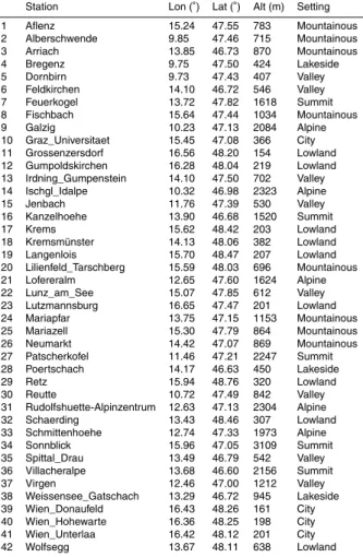
Table 1.Location, altitude and setting of the 42 meteorological stations used for calibration.

Station Lon (◦₎ _{Lat (}◦₎ _{Alt (m)} _Setting

1 Aflenz 15.24 47.55 783 Mountainous 2 Alberschwende 9.85 47.46 715 Mountainous 3 Arriach 13.85 46.73 870 Mountainous 4 Bregenz 9.75 47.50 424 Lakeside 5 Dornbirn 9.73 47.43 407 Valley 6 Feldkirchen 14.10 46.72 546 Valley 7 Feuerkogel 13.72 47.82 1618 Summit 8 Fischbach 15.64 47.44 1034 Mountainous 9 Galzig 10.23 47.13 2084 Alpine 10 Graz_Universitaet 15.45 47.08 366 City 11 Grossenzersdorf 16.56 48.20 154 Lowland 12 Gumpoldskirchen 16.28 48.04 219 Lowland 13 Irdning_Gumpenstein 14.10 47.50 702 Valley 14 Ischgl_Idalpe 10.32 46.98 2323 Alpine 15 Jenbach 11.76 47.39 530 Valley 16 Kanzelhoehe 13.90 46.68 1520 Summit 17 Krems 15.62 48.42 203 Lowland 18 Kremsmünster 14.13 48.06 382 Lowland 19 Langenlois 15.70 48.47 207 Lowland 20 Lilienfeld_Tarschberg 15.59 48.03 696 Mountainous 21 Lofereralm 12.65 47.60 1624 Alpine 22 Lunz_am_See 15.07 47.85 612 Valley 23 Lutzmannsburg 16.65 47.47 201 Lowland 24 Mariapfar 13.75 47.15 1153 Mountainous 25 Mariazell 15.30 47.79 864 Mountainous 26 Neumarkt 14.42 47.07 869 Mountainous 27 Patscherkofel 11.46 47.21 2247 Summit 28 Poertschach 14.17 46.63 450 Lakeside

29 Retz 15.94 48.76 320 Lowland

(17)

HESSD

12, 5055–5082, 2015

Title Page

Tables Figures

◭ ◮

Back Close

Full Screen / Esc

Discussion

P

a

per

|

Discussion

P

a

per

|

Discussion

P

a

per

|

Discussion

P

a

per

|

46°N 47°N 48°N 49°N

10°E 12°E 14°E 16°E

Met-Stations

Figure 1.Location of the meteorological stations used for calibration; coloured circles around

(18)

HESSD

12, 5055–5082, 2015

Title Page

Tables Figures

◭ ◮

Back Close

Full Screen / Esc

Discussion

P

a

per

|

Discussion

P

a

per

|

Discussion

P

a

per

|

Discussion

P

a

per

|

0 50 100 150 200 250 300 350

days of 2004 0

1 2 3 4 5 6 7 8

ET0 [mm/d]

a) ET0_p ET0_h

JAN FEB MAR APR MAY JUN JUL AUG SEP OCT NOV DEC 0

1 2 3 4 5

ET0 [mm/d]

b) ET0_p ET0_h

Figure 2.Daily time series of ET0 in 2004 for ET0 based on PM (ET0_p) and HM (ET0_h)

(19)

HESSD

12, 5055–5082, 2015

Title Page

Tables Figures

◭ ◮

Back Close

Full Screen / Esc

Discussion

P

a

per

|

Discussion

P

a

per

|

Discussion

P

a

per

|

Discussion

P

a

per

|

JAN FEB MAR APR MAY JUN JUL AUG SEP OCT NOV DEC 0.6

0.4 0.2 0.0 0.2 0.4 0.6 0.8

Bias [mm/d]

a)

0.4 0.6 0.8 1.0 1.2 1.4

RMSE [mm/d]

b)

Figure 3.Monthly Bias(a)and monthly Root Mean Square Error(b)between daily ET0_p and

(20)

HESSD

12, 5055–5082, 2015

Title Page

Tables Figures

◭ ◮

Back Close

Full Screen / Esc

Discussion

P

a

per

|

Discussion

P

a

per

|

Discussion

P

a

per

|

Discussion

P

a

per

|

0.002 0.003 0.004 0.005 0.006 0.007 0.008 0.009

Cadj

[-]

Grossenzersdorf Weissensee-Gatschach Rudolfshuette-Alpinzentrum

Figure 4.Monthly values ofC_adjat three different stations, the dashed black lines indicates the

(21)

HESSD

12, 5055–5082, 2015

Title Page

Tables Figures

◭ ◮

Back Close

Full Screen / Esc

Discussion

P

a

per

|

Discussion

P

a

per

|

Discussion

P

a

per

|

Discussion

P

a

per

|

0.4 0.6 0.8 1.0 1.2 1.4

RMSE [mm/d]

a)

20 40 60 80 100

RE [%]

b)

non-calibrated calibrated

Figure 5.Monthly Root Mean Square Error(a)and monthly Relative Error (b)between daily

(22)

HESSD

12, 5055–5082, 2015

Title Page

Tables Figures

◭ ◮

Back Close

Full Screen / Esc

Discussion

P

a

per

|

Discussion

P

a

per

|

Discussion

P

a

per

|

Discussion

P

a

per

|

2004 2005 2006 2007 2008 2009 2010 2011 2012 2013

0 50 100 150 200

ET0 [mm/month]

Grossenzersdorf 154 m.a.s.l.

2004 2005 2006 2007 2008 2009 2010 2011 2012 2013

0 50 100 150 200

ET0 [mm/month]

Weissensee_Gatschach 945 m.a.s.l.

2004 2005 2006 2007 2008 2009 2010 2011 2012 2013

0 50 100 150 200

ET0 [mm/month]

Rudolfshuette-Alpinzentrum 2304 m.a.s.l.

ET0_p ET0_h ET0_h.c

Figure 6.Monthly ET0 sums derived from ET0_p, ET0_h and ET0_h.c for three stations located

(23)

HESSD

12, 5055–5082, 2015

Title Page

Tables Figures

◭ ◮

Back Close

Full Screen / Esc

Discussion

P

a

per

|

Discussion

P

a

per

|

Discussion

P

a

per

|

Discussion

P

a

per

|

300 500 700 900 1100 1300 1500 1700 1900 2100 2300

Altitude [m]

0.001 0.002 0.003 0.004 0.005 0.006

Cadj

[-]

Figure 7.Monthly variations ofC_adjwith respect to altitude; the black contour line defines the

(24)

HESSD

12, 5055–5082, 2015

K. Haslinger and A. Bartsch Title Page Abstract Introduction Conclusions References Tables Figures ◭ ◮ ◭ ◮ Back Close

Full Screen / Esc

Printer-friendly Version Interactive Discussion Discussion P a per | Discussion P a per | Discussion P a per | Discussion P a per |

0 500 1000 1500 2000 2500 3000 3500 Altitude [m] 0.002 0.004 0.006 0.008 0.010 Cadj [-] JAN

0 500 1000 1500 2000 2500 3000 3500 Altitude [m] 0.002 0.004 0.006 0.008 0.010 Cadj [-] FEB

0 500 1000 1500 2000 2500 3000 3500 Altitude [m] 0.002 0.004 0.006 0.008 0.010 Cadj [-] MAR

0 500 1000 1500 2000 2500 3000 3500 Altitude [m] 0.002 0.004 0.006 0.008 0.010 Cadj [-] APR

0 500 1000 1500 2000 2500 3000 3500 Altitude [m] 0.002 0.004 0.006 0.008 0.010 Cadj [-] MAY

0 500 1000 1500 2000 2500 3000 3500 Altitude [m] 0.002 0.004 0.006 0.008 0.010 Cadj [-] JUN

0 500 1000 1500 2000 2500 3000 3500 Altitude [m] 0.002 0.004 0.006 0.008 0.010 Cadj [-] JUL

0 500 1000 1500 2000 2500 3000 3500 Altitude [m] 0.002 0.004 0.006 0.008 0.010 Cadj [-] AUG

0 500 1000 1500 2000 2500 3000 3500 Altitude [m] 0.002 0.004 0.006 0.008 0.010 Cadj [-] SEP

0 500 1000 1500 2000 2500 3000 3500 Altitude [m] 0.002 0.004 0.006 0.008 0.010 Cadj [-] OCT

0 500 1000 1500 2000 2500 3000 3500 Altitude [m] 0.002 0.004 0.006 0.008 0.010 Cadj [-] NOV

0 500 1000 1500 2000 2500 3000 3500 Altitude [m] 0.002 0.004 0.006 0.008 0.010 Cadj [-] DEC

Figure 8.Station-wise monthly third-order polynomial fit of the Hargreaves Calibration

(25)

HESSD

12, 5055–5082, 2015

Title Page

Tables Figures

◭ ◮

Back Close

Full Screen / Esc

Discussion

P

a

per

|

Discussion

P

a

per

|

Discussion

P

a

per

|

Discussion

P

a

per

|

(26)

HESSD

12, 5055–5082, 2015

Title Page

Tables Figures

◭ ◮

Back Close

Full Screen / Esc

Discussion

P

a

per

|

Discussion

P

a

per

|

Discussion

P

a

per

|

Discussion

P

a

per

|

Figure 10.Climatological mean annual sum of ET0 from 1961–2013(a); example of a daily

(27)

HESSD

12, 5055–5082, 2015

Title Page

Tables Figures

◭ ◮

Back Close

Full Screen / Esc

Discussion

P

a

per

|

Discussion

P

a

per

|

Discussion

P

a

per

|

Discussion

P

a

per

|

Figure 11.Upper panel: absolute anomalies of ET0 sum in July 1983(a)and July 1979(b)with

(28)

HESSD

12, 5055–5082, 2015

Title Page

Tables Figures

◭ ◮

Back Close

Full Screen / Esc

Discussion

P

a

per

|

Discussion

P

a

per

|

Discussion

P

a

per

|

Discussion

P

a

per

|

Figure 12. August 2003 monthly mean ET0 based on C_adj values – ET0_h.c(a), using the