The relationship between the general government debt and the gross domestic product: a case for Portugal

(1)

Department of Economics

THE RELATIONSHIP BETWEEN THE GENERAL

GOVERNMENT DEBT AND THE GROSS DOMESTIC

PRODUCT: A CASE FOR PORTUGAL

João Carlos Francisco de Almeida

Dissertation submitted as partial requirement for the conferral of Master in Economics

Supervisor:

Prof. Sofia Vale, Assistant Professor, ISCTE Business School, Department of Economics

(2)

Department of Economics

THE RELATIONSHIP BETWEEN THE GENERAL

GOVERNMENT DEBT AND THE GROSS DOMESTIC

PRODUCT: A CASE FOR PORTUGAL

João Carlos Francisco de Almeida

Dissertation submitted as partial requirement for the conferral of Master in Economics

Supervisor:

Prof. Sofia Vale, Assistant Professor, ISCTE Business School, Departament of Ecoomics

(3)

(4)

I

Acknowledgements

I would like to say a big thank you in first place to my supervisor Sofia Vale, who helped me through all this tasks, for all these years. It was a hard challenge for me, and there was several times were I was almost quitting; however she was always there to help me.

Another person that was absolutely one of the main factors to keep going with this dissertation was João Assunção, a friend for many years, who help me when I was completely lost.

To all my friends that were always amazing, tried to motivate me, and assured me that they will always be there for anything.

To my parents, who always supported me and I know that they always will.

I would like to dedicate this work to my father, who sadly could not observe the conclusion of this phase but I am sure that he would be proud of me for concluding it.

(5)

II

Resumo

Esta dissertação analisa empiricamente a relação entre o PIB, a dívida pública e o saldo da balança corrente em Portugal. Para este estudo foram usadas 37 observações anuais para um período compreendido entre 1980 e 2016.

Durante a crise financeira do ano de 2008 os níveis de dívida pública aumentaram de forma abrupta, tendo sido estes encarados como uma possível causa do abrandamento e a partir de certo nível decréscimo do PIB.

Recentemente, demonstrou-se que este efeito não existia em economias mais desenvolvidas. Contudo, o aumento dos níveis de dívida pública não deve ser fomentado, visto que proporciona uma maior volatilidade, sendo essa a razão pelo abrandamento do crescimento do PIB. Através de um modelo VECM foi possível verificar a existência de uma relação de longo prazo entre as variáveis. Adicionalmente, os resultados do teste de causalidade à Granger provaram não haver evidência de uma relação de curto prazo entre as variáveis.

Palavras-chave: Produto Interno Bruto, Dívida Pública, Portugal, VAR Classificação JEL: C32; H63; O40

(6)

III

Abstract

This dissertation analysis empirically the relationship between PIB, public debt and the current account balance in Portugal. In this study were used 37 yearly observations for the between comprehended between 1980 and 2016.

During the financial crisis of 2008, the levels of public debt raised sharply being considered one of the main factors for the slow growth or even decrease of GDP.

Recently, these effects were proven to be close to nil in advanced economies. However, the increase in public debt should not be stimulated, since it would lead to a higher volatility, which could be one of the reasons for slower GDP growth rates.

In a VECM model, it was possible to conclude the presence of a long-term relationship between the variables. Additionally, we had no evidence of Granger causality. Therefore, neither the public debt nor the current account balance could cause slow GDP growth rates in the short-run.

Keywords: Gross Domestic Product, Public Debt, Portugal, VAR JEL Classification: C32; H63; O40

(7)

IV

List of tables

Table 4.1 – Result from the stationarity and unit root tests, assuming the significance level of

10% ... 23

Table 4.2 – Result from the Lag Length Criteria done to the VAR model with LGDP, GGD and CAB ... 24

Table 4.3 – Autocorrelation LM Test with 4 lags ... 25

Table 4.4 – White Heteroskedasticity Test ... 25

Table 4.5 – Jarque-Bera Joint Test of normality of residuals ... 26

Table 4.6 – Number of cointegrating relations by model. Output E-views ... 26

Table 4.7 – Information Criteria by Rank and Model. Output E-views ... 27

Table 4.8 – Cointegration relationship ... 28

Table 4.9 – Granger causality... 30

(10)

VII

List of figures

Figure 1.1. – The non-linearity of the debt-growth relationship ... 3 Figure 2.1 – GDP (constant 2010 millions of US$) from 1980-2016. ... 13 Figure 2.2 – General government consolidated gross debt (percentage of GDP): Excessive deficit procedure (1980-2016). ... 14 Figure 2.3 – Current account balance (percent of GDP) 1980-2016. ... 15 Figure 4.1 – Impulse Response Functions. ... 29

(11)

VIII

List of abbreviations

ADF – Augmented Dickey-Fuller AIC – Akaike Information Criteria CE – Cointegration Equation EDP – Excessive Deficit Procedure EU – European Union

FPE – Final Prediction Error GDP – Gross Domestic Product

GMM – Generalized Method of Moments HQC – Hannan-Quinn Information Criteria IMF – International Monetary Fund

OECD – Organisation for Economic Co-operation and Development OLS – Ordinary Least Squares

PP – Phillips Perron

SIC – Schwarz Information Criteria VAR – Vector Autoregressive Model

(12)

1

Introduction

The debate between gross domestic product (GDP) and public debt has more than 50 years of existence, when in the beginning of the 1960s the idea that increases in public debt could have an impact on GDP growth rate was first suggested. However, this question remains unanswered until today. Is there a threshold for the level of public debt that jeopardizes GDP growth rate? Can a country feed GDP growth rate by increasing its own level of debt?

According to recent studies, high levels of public debt affect GDP growth, as Ahlborn and Scwickert (2015). However, public debt do not seem to have an impact in the GDP growth in advanced economies, as Panizza and Presbitero (2014) conclude.

Another question that is not yet answered is if there is a threshold for the levels of public debt above which GDP is compromissed. Reinhart and Rogoff (2010), Kumar and Woo (2010), Checherita and Rother (2010), Cecchetti, et al. (2011), Baum et al. (2013) and most recently Ahlborn and Scwickert (2015) defend the idea of the existence of a public debt threshold. The authors defined it as a turnaround point, after which the GDP growth would be significantly affected, even presenting negative growth levels.

However, Herndon et al (2013) confronted the idea of the existence of a threshold, when the author found that the impact was not too significant. Eberhardt and Presbitero (2013) added that the threshold could result of a misspecification in the model, while Pescatori et al. (2014) concluded that there is no threshold in such relationship.

Until now, this lively debate has produced some insights regarding the relationship of the two variables, and we can affirm that high levels of debt could lead to a situation where there is no capacity to repay their loans, contributing to lower GDP growth rates.

Since it is not clear if the high levels of public debt affect GDP growth and since economic systems may differ from country to country, we propose a study for a country that saw their accumulation of public debt rising sharply during the crisis and additionally that currently presents one of the highest debt-to-GDP ratios, in Europe, Portugal. This study uses a VAR model, to test for the presence of a long-term relationship between public debt and GDP between 1980 and 2016. In order to estimate the model, we have used unit root tests, lag length criteria, tests for the residuals of the VAR and cointegration tests. In a VECM model, with 2 lags, we have detected a long-run relationship between the three variables. Additionally we run

(13)

2

Granger causality tests and impulse response functions. In the Granger causality we could not prove that current account and public debt cause GDP in the short-run.

The organization of this dissertation is as it follows: in section 1 we will explain how the relationship between the two variables have evolved during the last fifty years. section 2 we will present the development of GDP, public debt and current account balance; section 3 will be dedicated to the methodology; section 4 will reflect the results of the model, and finally the conclusions.

(14)

3

Chapter I

– The relationship between public debt and economic

growth

Economists and policymakers currently assume that a high level of public debt can have negative effects on the economies of the countries, mainly due to two issues. The first one is the high volatility created when dealing with larger volumes of public debt. The second question raised was the fact that high levels of public debt could be correlated with a lower GDP growth. Due to the world crisis that peaked on the third trimester of 2008, this high level of public debt became a relevant academic, social and political topic largely because of growing concerns that the affected countries would not be capable of fulfilling their financial and economical responsibilities.

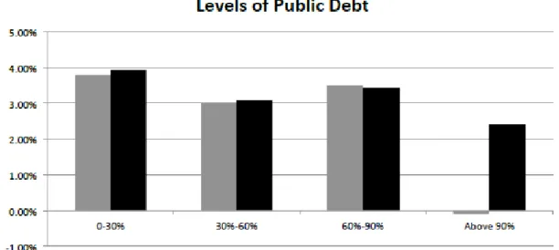
To find a solution for this concerning issue, several studies surged, led by the one from Reinhart and Rogoff (2010) that prompt a study that analyses the development of public debt and the long-term real GDP growth rate in a sample of 20 developed countries over the period between 1790 and 2009. The authors make two important conclusions. First, the relationship between government debt and long-term growth is weak for debt-to-GDP ratios below a threshold of 90% of GDP. Second, above 90%, the median growth rate falls by one percent and the average by more than three percent as shown in Figure 1 below.

Source: Reinhart and Rogoff (2010)

(15)

4

This work was of a big relevance, mainly because it was the first one that was published within the crisis verge, in a social and economic framework where governments were all searching for the best answer to their fiscal problems. Reinhart and Rogoff (2010) provided the first timely cues to the dreaded crisis questions. The study was of such significance that it inevitably led to a change in the implemented policies resulting in austerity measures. The authors confirmed the idea that began a few years earlier, that high levels of public debt have a negative effect on economic growth.

Modigliani (1961) was the first author suggesting that national debt could be a burden for future generations. This idea appeared at a time when Ricardian equivalence was generally assumed, national debt was not a problem for the economies and government expenditure, independently how it was financed. Before Modigliani, authors such as Buchanan (1958), Meade (1958 and 1959) and Musgrave (1959) had already questioned these ideas, although did not provide the adequate framework to do so. Modigliani concluded that an increase on the government purchase of goods and services, would lead to a higher national debt, which in normal situations would improve the economic welfare of present generations. Nevertheless, that increase would contribute to a higher debt and a burden for future generations, in the form of a reduced aggregate stock of private capital, which would lead to a reduced flow of goods and services. Just a few years later, Diamond (1965) divided the effects into two types of debt: internal and external public debt. The author studied the long-run competitive equilibrium in a growth model, and analyzed the effects created by the government debt. Diamond concluded that when the two types of debt were observed, internal debt would increase the interest rate, and contribute to a lower utility. In terms of external debt, that would force interest rate and the growth rate to take opposite directions. Furthermore, the author concluded that substituting internal for external debt would lead to an interest rate rise and to a lower utility. The author added that taxes directly reduce the available lifetime consumption of a certain individual taxpayer and this would contribute to a lower disposable income, diminishing individual savings and thus to a reduction in capital stock.

Both Saint-Paul (1992) and Aizenmann (2007) used an endogenous growth model to study the relationship between public debt and growth. The authors presented similar results where both assumed that an increase in public debt would reduce the country’s growth rate. The solution presented by the authors was to maintain a constant debt-to-GDP ratio to avoid lower GDP growth rates.

(16)

5

Even though they share similar results, the specifications of the models were different. Saint-Paul (1992) extended the Blanchard (1985) model, by assuming the existence of an externality which suggests constant returns to capital at the aggregate level. The author claimed that contrary to the classical model that compares the interest rate with the growth rate, the endogenous model with externality differentiates between the social and the private rate of return. Saint-Paul concluded that for production efficiency the pertinent rate of return was the social one, and the author demonstrated that it surpassed the growth rate, and so the economy would be production-efficient. In terms of consumption efficiency, the appropriate one was the private rate of return, and the author proved that the economy might be dynamically inefficient. With this result it was not expected an increase in public debt allocation, because the interest rate did not change. Instead, it would reduce the growth rate, and so in the future, there would be a generation with reduced welfare.

Aizenman et al. (2007) analyzed the fiscal policy and optimal public investment for nations characterized by restricted tax and debt capacities. One of the authors conclusions was that different public finance constrains could be one of the reasons for different growth rates across countries. Moreover, the flow of public expenditure would increase productivity of both capital and labor, but borrowing to finance it was not advisable since it would increase public debt that reduces both welfare and growth rate.

Krugman (1988) trying to explain how to deal with countries with external debt problems, discusses the choice between debt financing vs. debt forgiving and comes out with the term ‘debt overhang’. Whenever countries’ expected repayment ability of their external debt is below their real value of debt they are facing a debt overhang. According to the author, the decision between financing or forgiving should not be made only on the debate between liquidity vs. solvency. This debate should signify a tradeoff between the value of a large amount of debt and the expected incentive effects of a debt that is improbable to be repaid. If creditors have some hope that the country can repay its debt, it should not be forgiven. In the case where only in exceptional circumstances the debt will be paid, some part of debt should be forgiven, to increase the possibility of remaining debt repayment.

More recently, Panizza and Presbitero (2013) wrote a survey compiling both theoretical and empirical works, which study the relationship between public debt and economic growth in advanced economies. Their first remarks were that the causal effect issue between high debt and low growth was not debated until then and an analysis was necessary. Moreover, the authors

(17)

6

showed that the evidence of a debt threshold, in which once surpassed the growth rates fall, is not robust across samples, estimation techniques and specifications. However, the high levels of debt should not be ignored as these could represent a major problem and could harm economies. According to Panizza and Presbitero (2012) countries with high levels of debt may consider restrictive fiscal policies a way of diminishing unexpected reactions from investors. Nevertheless, this solution should not be implemented in the middle of a crisis but as a preventive measure. Cottarelli and Jaramillo (2012) affirmed that these restrictive policies, with the intention of reducing the high levels of debt in the long-term, might reduce growth in the short-term and the effects could be devastating when applied in a period of crisis.

Cecchetti et al. (2011) raised some questions about this thematic. Why did we reach to such high levels of public debt? Is there any level of debt that after which economic growth is negatively affected? According to Woodford (1990) the first question could be answered by the simple fact that liquidity services are provided by government debt in order to facilitate credit conditions to the households – since the government can access liquidity at a considerable lower rate than the other economic units. This would lead to a higher public debt, which would induce higher capital in the private sector, with this one being capable of giving the proper answer when variations occur both in the investment opportunities and in income variables. Thus, borrowings allowed individuals to smooth their consumption, corporations to smooth investment and production and finally government to smooth taxes. This inevitably contributed to rising debt and financial deepening that lead to improvements in economic welfare. The second question is a bit harder to answer, but it was answered by some empirical frameworks, that found different levels of debt-to-GDP, levels in which the effect became negative.

An overview on the empirical studies about this subject indicates that often authors conclude that there is a non-linear impact of external debt on growth, where the negative effects are observed only after a certain debt-to-GDP ratio threshold.

Pattillo et al. (2002) use a dynamic panel data model of 93 developing countries in the period comprehended between 1969 and 1998, where they have made three main conclusions on this purpose. First, the authors conclude that debt seems to have a nonlinear effect on growth, but based on their results there was no possibility to precisely estimate that relation. The other relevant conclusion is that over 35-40 percent of GDP debt appears to have a negative impact on per capita growth. The author’s third conclusion on the grounds of an “inverted-U”

(18)

7

relationship between external debt and growth will be analyzed later, in contrast with Schclarek (2004).

Schclarek (2004) used a dynamic system Generalized method of moments (GMM) panel estimator, containing 83 developing and industrial countries between 1970 and 2002. The author studied both the linear and nonlinear relationship between debt and economic growth, obtaining two types of results. In terms of developing countries, the author finds a negative impact of external debt on economic growth. Furthermore, the author divided public external debt and private external debt, concluding that there is a negative relationship between public external debt and growth, but there was no evidence when considering the private external debt. When considering developing countries there is a notable contrast between the results found by Patillo et al. (2002) and the results in Schclarek (2004). The first find statistic significant results of a nonlinear relationship between total external debt and growth. Additionally, there is a positive relationship between the two of them when the external debt level appears below a certain threshold, and a negative relationship when it’s above the threshold, a “so called” inverted-U relationship. In divergence, Schclarek (2004) only appears to be in accordance to the nonlinear relationship, finding that there is no evidence of this positive relationship, and no indication of this inverted-U described by Patillo et al. (2002).

In terms of industrial countries, it was not found a robust and statistically significant evidence between gross government debt and economic growth. This would suggest that, in fact, higher public debt does not have to be correlated with a lower GDP growth rate.

After the publication of Reinhart and Rogoff (2010), some authors as Kumar and Woo (2010), Checherita and Rother (2010), Cecchetti et al. (2011) and Baum et al. (2013) tried to confirm the results presented in Reinhart and Rogoff’s paper. The results presented pointed to a nonlinear relationship between debt and growth, and the appearance of a negative effect between 85 to 100% of debt-to-GDP threshold.

Kumar and Woo (2010) used a panel of 38 advanced and emerging countries in the period of 1970-2007. The authors concluded that above 90% threshold, the effects became negative and the impact was different in emerging and advanced countries. In the first ones, a 10-percentage point increase in the initial debt-to-GDP ratio would lead to a 0.2 percentage points per year reduction in annual real per capita GDP growth, while in advanced countries the impact is about

(19)

8

0.15 percentage points. Furthermore, the authors recommended reducing the public debt in the medium and long term to avoid problems with growth.

Checherita and Rother (2010) explained growth as a quadratic functional form of debt in a sample of twelve-euro area countries in the years between 1970 and 2011 and found significant evidence of an inverted U relationship, like the one presented by Pattillo et al. (2002). The authors claim that a negative relationship was found above 90 to 100% debt-to-GDP threshold and enhance this analysis by stating that this problem might begin at 70% of GDP.

Cecchetti et al. (2011), analyses the debt effect for 18 Organisation for Economic Co-operation and Development (OECD) countries in the period comprehended between 1980 and 2010, providing new conclusions for the empirical literature. Their study is extended to corporate debt and household debt. Nevertheless, the analysis for the government debt is similar to the previous studies where they found that the threshold was near 85% of GDP, and a 10-percentage point increase would indicate a 0.1-percentage point decrease in growth while Kumar and Woo (2010) registered a 0.15-percentage point decrease. Relating to corporate debt, the threshold is close to 90%, and the impact is approximately half comparing to the results observed concerning government debt. In terms of household debt, the results were not statistically significant but the authors project a threshold of 85%. The solution presented by the authors is to try to keep debt below these levels of threshold.

In Baum et al (2013) paper, the authors pick up 12-euro area countries from 1990-2010. The authors studied the short-term impact of debt on GDP growth and concluded that there is a positive impact, but that after 67% debt-to GDP ratio, this impact is almost zero and is not significant. Furthermore, once again the same results are presented: debt above a 95% threshold has a negative impact on economic growth.

Beyond the discussion, Herndon et al (2013) presented completely different results from the previous ones. The authors tried to obtain the same results as in Reinhart and Rogoff (2010), where the authors found that the results had errors in the importance given to the debt variables as well as some mistakes in processing information; the database used had some limitations such as excluded data and other information gaps. All these problems lead to multiple inaccuracies found in the results of Reinhart and Rogoff (2010). The authors contradicted the opinion that economic growth really differs below and above a 90% threshold. Their conclusion pointed to a different vision from those previously presented: the authors argue that the turning

(20)

9

point begins near 120% of debt, and that even with this high level, the effects are not as vast as presented in prior studies.

As we can imagine, this study, presenting such different results, had some consequences on the way of thinking about this topic, and consequently led to several other studies and to the inevitable questioning of the 90% threshold presented until then. With these conclusions from Herndon et al. (2013), a new era could be beginning. As examples of these further studies there are authors such as Eberhardt and Presbitero (2013) and Pescatori et al. (2014) that pointed that there is no evidence of the threshold discussed in previous papers.

Eberhardt and Presbitero (2013) in their first analysis found that there are differences in the relationship between debt and growth across countries, and that the nonlinearity was not found in a within-country analysis. Furthermore, the authors concluded that the long-run debt coefficients seem to be smaller in countries with a higher debt, even if the average long-run debt coefficient was still positive. The second relevant conclusion was the use of a linear specification contrary to the most commonly used polynomial specification. They used pre-specific thresholds, and find that the debt coefficient in the thresholds vary positively in some, and negatively in others, which will mean that it would vary from country to country. With these conclusions, the thought that the 90% threshold was a result of an empirical misspecification gained substance.

Pescatori et al. (2014) found that there is no threshold for debt ratio above which the growth could be compromised. On their studies the relationship between debt and growth at higher levels even becomes weak, when focusing on a short-run relationship. Another important conclusion was that countries with high levels of debt, but in which the debt is declining, have been growing without problems. Nevertheless, the authors affirmed that debt is important in a way, that the higher the level, the higher the volatility and this could lead to problems in economies.

The most relevant empirical work was made by Panizza and Presbitero (2014), where they study if the public debt has a causal effect on economic growth in a database of 17 OECD countries covered in the sample used by Cecchetti et al. (2011). This study could not provide a concrete answer about the question made. However, the authors found that, in the medium run, the high levels of public debt are not responsible for a lower growth in advanced economies. They add that with this result the relationship between debt and growth should not be an explanatory way of fiscal consolidation. But once again, as in Pescatori et al. (2014), the authors mention that

(21)

10

the level of debt is important to control to avoid ‘debt overhang’. In conclusion, further studies should be made to study the causal effect of public debt on economic growth.

Bearing in mind that the literature referring to the causal effect between the two variables was scarce, Puente-Ajovin and Sanso-Navarro (2015) developed an empirical work based on the article of Cecchetti et al. (2011) to study the Granger causality between debt and growth in 16 OECD countries. One of the main ideas was that in fact, lower growth rates lead to a rise in the debt-to-GDP ratio in the short run. Another result suggested that higher (non-financial) private indebtedness levels Granger causes slower growth with special attention to the household debt. The authors recommended that a framework of causal relationships should be used to determine policies in the short run, to improve economic circumstances. Nevertheless, policymakers should be careful when reducing the levels of public debt during a recession, as the non-causal relationship from public debt to growth was not proved yet.

Ahlborn and Scwickert (2015) proposed another type of analysis of the “so called” threshold. Until then, other authors (in general) had assumed homogeneous debt effects across their samples. Ahlborn and Scwickert used two approaches. The authors used a panel data of 111 OECD and developing countries in order to study the homogeneous public debt threshold. The authors presented two thresholds where the negative debt effects appear, one between 76 and 86% and the other between 96 and 105% of GDP. Even though the presented results were like the ones in Reinhart and Rogoff (2010) where the threshold was around 90% of GDP some questions aroused. The no significant estimator between 86% and 96% could be a result of the cross-country heterogeneity between debt and growth, and could in fact signify that some countries would still handle such high levels of debt-to-GDP ratios.

The authors then formed three clusters (Continental, Nordic and Liberal) based on their economic systems’ differences. In terms of the Continental country group, the authors found that the negative debt effects begin at around 70% and that the effects are more noticeable after 75%. In the Nordic group most of the threshold values analyzed was not significant, but after 60% the negative debt effect kicks in. Nevertheless, most of the Nordic countries stayed below that threshold value in most of the sample. Finally, considering the Liberal group, the results presented by the authors were that high levels of public debt do not have a negative impact and this impact could even be positive in the long-term. In conclusion, these results present us the differences in the economic systems and contribute to a different relationship between public debt and economic growth.

(22)

11

As it was seen in the empirical frameworks, this facilitation of credit started to go in the wrong way, when some borrowers’ ability to repay their loans was insufficient because of the high levels of accumulation of debt. This contributed inevitably to real volatility, increased financial fragility and consequently led to a reduction on average growth. As Eggertson and Krugman (2011) describe, a decline in aggregate demand is a result of an asymmetry between the highly indebted ones and the ones that are not. They advise that to fill the gap that appeared due to this situation, an intervention should be made by the public sector. The problem is that the public-sector funds are limited, and in a situation of crisis this may affect in such level that the public sector will not have capacity to fulfill this gap and simultaneously do their essential government functions.

The analysis that can be made by the most recent empirical frameworks is that even though high levels of debt would not lead directly to a reduce in economic growth, the growing debt contributes to a higher volatility in the economies, and that could create a reduction in the economic growth.

(23)

(24)

13

Chapter II

– The EU crisis and the impact in Portugal

In the last few years, the world faced one of the biggest financial crisis in history. This worldwide crisis had repercussions in many countries and led to the implementation of fiscal policy austerity measures. This was also the case of the European Union (EU), which suffered the consequences of a credit boom in all the sectors of the economy. Because of the crisis, the public sector assumed a significant part of the sector private responsibilities, namely from the banking industry, leading to the explosion of public debt. However, one of the major problems brought about by the financial crisis was the decrease of GDP per capita growth rates that spread all over Europe. Since our mainly concern is to analyze the case of Portugal we will present the evolution of GDP, Public Debt and Current account balance. Additionally, since Public debt and Current Account balance ratios were calculated using US dollars, the variable GDP will be presented in US Dollars.

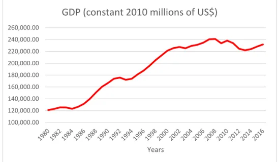
Figure 2.1 – GDP (constant 2010 millions of US$) from 1980-2016. Source: World Bank Data

Figure 2.1 presents the annual Gross Domestic Product with constant 2010 US dollars prices between 1980 and 2016. In the beginning of the 80’s, Portugal was suffering a severe crisis, which lead to an intervention from International Monetary Fund (IMF) during the year of 1983, a loan of 750 million of US dollars. This crisis, lead to the decrease in the amounts of GDP from approximately 125,556 in 1982 to 122,983 million of US dollars in 1984. After that period of crisis, Portugal had a steady growth until the year of 2009 (exceptions made for the years of

100,000.00 120,000.00 140,000.00 160,000.00 180,000.00 200,000.00 220,000.00 240,000.00 260,000.00 Years

(25)

14

1993 and 2003 were there was a decrease in GDP). From 2009 until 2013, Portugal presented a decrease in the GDP amount in four periods, which demonstrates that the country faced an austere crisis. During this period, another intervention by the IMF occurred (2011), this time with a loan of 116,000 million of US dollars. In 2014, Portugal started slowly recovering from the dark years faced before presenting a stable growth during the following 3 periods. However, the GDP for 2016 (231,745 million of US dollars) is still below the GDP levels presented in 2008, were the amount was 241,041 million of US dollars.

Since we have observed that Portugal had interventions by the IMF in both 1983 and 2011, it is important to analyze the evolution of the public debt since the high levels of public debt may have influence in GDP growth as we have stated before.

In order to avoid growing levels of debt and to correct excessive deficits, the European Commission adopted the Excessive Deficit Procedure (EDP). The main objective of this procedure was to act in countries, which have at least of the following issues:

 Government debt to GDP ratio surpassed 60%;  Deficit was higher than 3%.

Despite the efforts in order to maintain the stability of public levels, these increased in several countries during the past few years.

Figure 2.2 – General government consolidated gross debt (percentage of GDP): Excessive deficit procedure (1980-2016). Source: AMECO 0 20 40 60 80 100 120 140 Years

General government consolidated gross debt

:-Excessive deficit procedure (based on ESA 2010)

(26)

15

Figure 2.2 above shows the evolution of general government debt based on EDP in percentage of GDP from 1980 until 2016. As we have mentioned before, during this period IMF had two interventions in Portugal, which coincide with the periods where the accumulation of debt was higher. Between 1980 until 1985, the general government debt went from 29.09% to 55.66% of GDP respectively. Afterwards, until 2003 this ratio maintained relatively stable between 50% and 60% of GDP. From 2003 until 2008, there was a steady growth in this ratio, which brought the ratio from 58.63% in 2003 to 71.66% in 2008. However, during the period from 2008 until 2012, which once again coincided with another IMF intervention, this ratio had augmented an impressive 54.56 percentage points, reaching 126.22% of GDP in 2012. Since then the ratio had stabilized, corresponding to 129.86% of GDP in 2016.

Furthermore, it would be interesting to observe the current account balance, which represents the countries’ transactions with foreign countries and the external financing that the countries receive from abroad. This balance includes the net trade in goods and services, net transfer payments, and investments.

In order to understand if the accumulation of debt and the slow GDP growth is related with negative current account balances we will proceed with the analysis of this variable.

Figure 2.3 – Current account balance (percent of GDP) 1980-2016. Source: IMF

Figure 2.3 above, represents the current account balance in percentage of GDP for Portugal between 1980 and 2016. As we expected, Portugal presented deficit in terms of the current

-16.00 -14.00 -12.00 -10.00 -8.00 -6.00 -4.00 -2.00 0.00 2.00 4.00 Years

(27)

16

account balance in several years, aggravating once again during the two crisis. Between 1980 and 1984, Portugal had five consecutive years were the current account balance was negative, including two years (1981 and 1982) in which the balance was -14.4 and -10.6 % of GDP. From 1985 until 1993, Portugal showed the most stabilized years in terms of this balance were the percentages were close to zero. The highest current account balance percentage was during this period with 3.1% of GDP. After 1993, Portugal presented 19 consecutive periods were this balance was negative, including six years were the balance presented a deficit of over 10% of GDP. The turning point was the year of 2013, were Portugal presented a surplus of 1.6% of GDP, the highest in 28 years. The three following periods maintained the surplus of this balance even though the percentages were close to zero.

In terms of conclusion to the analysis of these variables, we observed that the two existing crisis in Portugal, during the 1980s and the end of the beginning of the 2010s lead to slow GDP growth, an uncontrollable accumulation of debt, and several periods where Portugal had a negative current account balance.

Does the negative current account balances could explain the high accumulation of debt? Does the high levels of debt could explain slower GDP growth rates and even negative ones?

From the analysis of the variables above, we can affirm that Portugal’s deficit current account balance, lead to a necessity of external financing and indirectly could have guided to an accumulation of debt. The second question is the so-called million dollars question, since the researchers have not found yet an answer. However, the period where the accumulation of debt was higher coincided with the period of lower GDP growth rates.

We will propose a study with the concerning variables in order to understand the relationship between themselves.

(28)

17

Chapter III

– Methodology

The most recent economic crises, which peaked in the third quarter of 2008, created a completely new debate relating public debt and GDP, since investigators questioned if the continuous accumulation of public debt could be one of the major factors for lower GDP growth rates. Reinhart and Rogoff (2010) opened the discussion, leading to several articles being published in the following years, where the focus was to try to understand the relationship between both variables. Does the public debt affect GDP? That is the question that we pretend to answer with this study.

We propose a Vector Auto Regression model (VAR model) analysis. We will proceed with stationarity and cointegrations tests, Granger Causality test and the impulse function response to understand the relation between public debt and GDP.

VAR model option was chosen over other models since it assumes that all the variables are endogenous and in this context, it makes sense because it would avoid making assumptions regarding whether the variables are endogenous or exogenous. Additionally the model would allow us to check if a long-term relationship exists, to test the causality between themselves and to observe the impact produced by shocks.

This model presents one equation for each variable, which means that in the case where three variables are included ( _𝑡, _𝑡 and _𝑡), three equations will be presented. The variables should be explained by their own lagged values, the lagged values of all the other variables and an error term. In our example, _𝑡 will be explained by their own lagged values, the lagged values of _𝑡 and _𝑡 and an error term.

Brooks (2008) defines that the simple case of a VAR model with two variables _𝑡 and _𝑡 can be described by the following equations:

𝑡 = + 𝑡− + ⋯ + 𝑡− + 𝑡− + ⋯ + 𝑡− + 𝜇 𝑡 (1)

𝑡 = + 𝑡− + ⋯ + 𝑡− + 𝑡− + ⋯ + 𝑡− + 𝜇 𝑡 (2)

(29)

18

The VAR models have several benefits when compared with other models such as:  All the variables are endogenous;

 Each variable is explained by their own lagged values and the lagged values of all the other variables included in the model;

 Possibility of using Ordinary Least Squares (OLS), since all the right side elements of each equation are pre-determined at time t;

 Better performance in terms of forecasting compared to large-scale structural models. However, VAR models have some limitations as:

 These models are not based on or concerned with theory, in this sense they could be structured in an incorrect way leading to misleading results;

 All the variables should be stationary.

 The number of parameters. If per example we include three variables and three lags, the number of coefficients to calculate will be thirty.

 How to determine the number of lags that should be included in the model?

In order to deal with these limitations we will proceed with some tests in order to mitigate the risks. Regarding the first presented limitation, we will study the relationship between public debt and GDP, a debate that has decades of existence. For the second limitation, we will proceed with some stationarity and unit roots tests, in order to determine the stationarity of the variables, which will be explored in chapter 3.1. To deal with third and fourth limitations, we will restrict the number of parameters by introducing three variables, while the number of lags will be determined using lag length criteria, which will be on focus in chapter 3.2

3.1. Stationary test

The unit root tests consist on testing the integration order of yt, which means, the number of

differences needed to get a stationary yt. Wooldridge (2002) defines a stationary series,

integrated of order 0 I(0), has a series which probability stays stable over time, in this sense, if we select a group of random variables in a sequence and change this sequence for t time periods, the joint probability should stay the same.

The selected tests for this analysis were the Augmented Dickey-Fuller (ADF) test and the Phillips Perron (PP) test. These two tests can present the following results:

 Stationary I(0), without stochastic trend;  Stationary with a stochastic trend;

(30)

19

The main difference between the first two results can be explained by the fact that the second is not a stationary process per se, which can be transformed in a stationary process by removing the associated trend.

In the case that the test determines a non-stationary process, the processes could be converted into stationary by applying the first differences. However, the author does not recommend this method, since using it will lead to losing important information for the long-term analysis of the VAR.

The ADF test presents us with two hypotheses. The null hypothesis is that the series has a unit root. If we do not reject the null hypothesis (H0), the series is considered non-stationary and

that means that it has a unit root. In contrast, if we accept the alternative hypothesis H1 we can

have that the series is stationary. Additionally, if the second is true, the series could have a stochastic trend or not.

The ADF test could be represented by the following equation: ∆ 𝑡= + 𝑡− + ∑= ∆ 𝑡− + 𝜀𝑡 (3)

Where,

 y is the time series;  is the drift parameter,  ∆ is the difference operator,

 and are parameters to be estimated,

 𝑘 is the lag value which ensures 𝜀𝑡 white noises series

The decision method to choose to accept or reject H0 is based on the analysis of the p-value.

There are three levels of significance that can be used (10%, 5% and 1%), however the most common is the 5%, which we will be based on. If the p-value is higher than 5% we do not reject H0 . By the opposite, if it is lower than 5% we will reject H0 and we will accept H1.

The PP test can be defined by the following equation: ∆ 𝑡= + 𝑡− + 𝜀𝑡 (4)

This test will serve as confirmation test of the ADF test. The difference from this to the ADF test, is that PP makes a non-parametric correction to the t-test. The hypothesis for this test act in the same way as ADF test.

(31)

20

3.2. Lag Length Criteria

Lag Length Criteria for a time-series is a crucial econometric exercise to select the lag length. The VAR is a dynamic model based on past periods that obliges us to determine the number of lags to introduce in the model.

The Lag Length tests provides us with five different criteria that can be chosen to determine the number of lags in the model; the sequential modified LR test statistic; final prediction error (FPE); Akaike information criteria (AIC); Schwarz information criteria (SIC); Hannan-Quinn information criteria (HQC).

Liew (2004) suggest the usage of FPE and AIC in models where the number of observations is lower than 60. Additionally, the author suggests that in models with over than 120 observations the most appropriate criteria would be HQC.

3.3. Vector error correction model and cointegration

Brooks (2008) defines VECM equation as the following:

(5)

Where, = ∑ ₌ − _𝑔, = ∑ ₌ − _𝑔, g the number of variables, k the number of lags, a coefficient matrix and a long-term coefficient matrix.

A VECM model is a model in which both variables are non-stationary in levels, but are integrated of the same order. Being integrated of the same order, the variables could be tested in order to analyze if there is any cointegration relationship.

The cointegration relationships are the ones responsible for the long-term relationship between two or more variables. Hamilton (1994) explains that this relationship can only exist with I(1) series - series which individually diverge in a random way, though there is a linear combination within this series that can form a stationary process.

In this sense, if we have two variables _𝑡 and _𝑡 in which case they are both I(1), a cointegration relationship is possible if _𝑡+ _𝑡 combined are I(0) and both a and b are different from 0. The most commonly use cointegration test is Johansen test which analyses the long-term coefficient represented in equation 5 by . This test, despite being more complex than the others, determines the exact number of cointegration vectors, which could be more than one.

(32)

21

The Engle-Granger and Phillips-Ouliaris tests only verify if the variables are cointegrated and assume a unique cointegration vector.

While applying this test, one has to choose the determinist trend assumption of the test. The following options are available:

 No deterministic trend in data:

o_{No intercept or trend in Cointegration Equation (CE) or test VAR;} o_Intercept– no intercept in VAR;

 Linear deterministic trend in data: o Intercept in CE and test VAR;

o Intercept and trend in CE – no intercept in VAR;

 Quadratic deterministic trend in data with intercept and trend – intercept in VAR;  Summary of all the tests.

To choose the appropriate deterministic trend assumption of the test, we will use the option of summarizing all the tests in order to have a wider view of all the possibilities. We will choose the number of cointegration relations based on the Trace and the Max-Eig, and additionally we will confirm these relations with the Information Criteria (Akaike Information Criteria and Schwarz Criteria), which will provide both the appropriate Rank (the number of cointegration vectors) and the model.

Since both tests (Trace and Max-Eig) test the cointegration vectors (r) we have the following hypothesis:

: 𝑟 = : < 𝑟 ≤ 𝑔 : 𝑟 = : < 𝑟 ≤ 𝑔 : 𝑟 = 𝑔 − : 𝑟 = 𝑔

Where g represents the number of variables. The in the first test represents no cointegration vectors and therefore would be zero rank. If is rejected, the further tests will be run until determining the number of cointegration vectors. If r=g, we can deduce that in fact has full rank, and consequently _𝑡 would be stationary, which will take us back to the VAR analysis. Since r, determines the rank of , is a product of two matrixes and can be defined has:

(33)

22

Where, are the adjustment parameters, or by other words the corresponding coefficient to each cointegration vector. ′ are the cointegration vectors. If we consider g=3 and r=1 then the

matrix is written by: = 𝛼𝛼

𝛼 (7)

3.4. Granger Causality

The Granger Causality test purpose is to verify the short-term causalities between the variables in terms of forecasting. With this method, we will be able to verify if any variable can help to determine others, and if GDP has any influence in determining Public Debt, or vice versa. If we pick two variables _𝑡 and _𝑡 we can expect from this method two different results:

 H0 mean that _𝑡 does not Granger-cause _𝑡;

 Rejecting H0 mean that _𝑡 Granger-cause _𝑡.

The intuition explains that if we reject H0, _𝑡 predictions are better when using _𝑡 and _𝑡 past

values, rather than only using _𝑡 past values.

3.5. Impulse Response Function

The impulse response function is a methodology used to verify the capability of response by the dependent variables when hit by exogenous shocks. In this sense, the effect of these shocks could be detected in long-term. In other words, this methodology is used to analyze the behavior of the variables in a dynamic process system.

If the response to a shock is always null by the dependent variable, this means that there is no cause-effect. In contrast, if we detect a negative reaction in the dependent variable ( ) by a change in an independent variable ( ), we can deduce that a shock in ( ) will have a negative effect in ( ).

Since the order of the variables is relevant having an impact on the responses, we will use the decomposition method by Cholesky.

(34)

23

Chapter IV

– Empirical Results

4.1. Data

Since 2010, several articles were published with empirical analysis concerning the relationship between GDP and general government debt. Meanwhile, we decided to choose a country that was massively affected with the crisis of 2009, Portugal.

The chosen period for analysis was from 1980 until 2016 with yearly data, and the variables were the following:

 Gross Domestic Products at constant prices of 2010 from World Bank national accounts data and OECD National Accounts data files;

 General government consolidated gross debt (GGD), percent of GDP:- Excessive deficit procedure (based on ESA 2010) from AMECO and;

 Current account balance (CAB), percent of GDP from IMF.

We have converted GDP into its natural logarithm and let the other two variables as ratios.

4.2. Stationarity and Unit roots

This test will determine the type of model that will be used further on. If all the variables are stationary in levels, we should use a VAR model. In contrast, if all the variables are I (1), we should use a Vector Error Correction Model (VECM).

Table 4.1 – Result from the stationarity and unit root tests, assuming the significance level of 10%

Table 4.1 presents the p-values for the variables both in levels and first differences. The tests for all of the variables in levels presented p-values above 5%, which mean that we cannot reject

, and that the variables have a unit root.

Variables Unit Root Intercept Trend & Intercep Intercept Trend & Intercep

Level 0.39 0.85 0.35 0.98 First Differences 0.08 0.14 0.08 0.11 Level 0.94 0.72 0.98 0.95 First Differences 0.06 0.09 0.06 0.12 Level 0.42 0.78 0.35 0.71 First Differences 0.00 0.00 0.00 0.00 Period: 1980-2016 LGDP GGD CAB ADF PP

(35)

24

We then proceed with the test to the first differences of all the variables. The tests for CAB show that the variable is stationary in first differences with a p-value lower than 5%, while both LGDP and GGD present p-values higher than 5%. However, if we accept a 10% level of significance, both LGDP and GGD have a stationary process considering only Intercept, with p-values of 0.08% and 0.06% respectively.

Since all the variables are I (1) and diverge randomly on time, we can proceed with the study of cointegration. Additionally, this means that a long-term relationship is possible between the variables and that we will be using a VECM model.

4.3. Lag Length Criteria

We have tested a first VAR model, to determine the optimal number of lags to include. In this model, we have included the logged GDP, GGD and CAB.

To choose the most appropriate criteria to use we recurred to Liew (2004), which determines the best criteria based on the number of observations. Since we have 35 observations we will use FPE and AIC tests.

Table 4.2 – Result from the Lag Length Criteria done to the VAR model with LGDP, GGD and CAB

As we can observe from the table above, both tests (FPE and AIC) indicate the optimal lag length as two lags. Regarding the other criteria, we can conclude that all define 2 as the fitting number of lags, expect SIC that defines that the number of lags should be 1.

4.4. Residuals Tests

After defining the lag length as two lags, we will analyze the residuals in the VAR model, recurring to three tests. One related with serial correlation, other related with heterokedasticity and the last one with the normality of the residuals. In order to validate the model, we should perform these tests to despite any malformation in the structure of itself.

Lag LogL LR FPE AIC SC HQ

0 -220.3544 NA 151.8741 13.53663 13.67267 13.58240

1 -65.47675 272.2091 0.022049 4.695561 5.239745* 4.878662 2 -52.45377 20.52106* 0.017558* 4.451743* 5.404066 4.772171* 3 -49.24147 4.477741 0.025934 4.802514 6.162975 5.260267 4 -36.99789 14.84070 0.022992 4.605933 6.374533 5.201013

(36)

25

Serial correlation could be defined has the relationship between various observations over specific periods of time in each variable. In other words, this will mean that future values are not independent of past values, which will lead to a pattern in the given variable. For VAR models, we will need to avoid serial correlation.

Table 4.3 – Autocorrelation LM Test with 4 lags

In order to test serial correlation, we used the Autocorrelation LM Test, which full results can be observed in Annex A1. Has we can observe from table 4.3 above, the p-value is higher than 5%, being 0.066, which means that we cannot reject the null and that the model has no serial correlation problems.

Heteroskedasticity could be defined has nonconstant standard deviations of a variable over specific periods of time. The problem of heteroskedasticity can be seen in variables as bonds or stocks since we cannot predict their volatility. In this sense, we need to have a model where the variance is stable, which can be called homoscedastic.

Table 4.4 – White Heteroskedasticity Test

In order to test if the residuals are heteroskedastic, we used the White Heteroskedasticity test which full results can be observed in Annex A2. Has observed in table 4.4, the p-value is higher than 5%, being 0.2537, which means that we do not reject for homoscedasticity.

The third test to the residuals is the Normality Test. If we do not have a normal distribution, we will have to run a non-parametric test, or verify our data for outliers, or multiple distributions combined, or we may have insufficient data.

Autocorrelation LM test

H₀: No autocorrelation within the residuals H_1:Autocorrelation within the residuals 16.04186 (p-value: 0.066)

White Heteroskedasticity Test (no cross terms)

H0: Homocedasticity

H1: Heteroskedasticity

(37)

26

Table 4.5 – Jarque-Bera Joint Test of normality of residuals

We have used the Lutkepohl test with Cholesky of covariance in order to test the distribution of the residuals which full results can be observed in Annex A3. Has observed in Table 4.5, by the Jarque-Bera Joint Test we can accept with a p-value of 0.8466.

4.5. VECM Model and Cointegration

After defining the number of lags as 2, following the criteria above, we run the Johanssen Cointegration Test.

The decision of the number of cointegration vectors and which type of model to use in the VECM model, will be based both on the Trace and Max-Eig tests.

Table 4.6 – Number of cointegrating relations by model. Output E-views

Table 4.6 above represents the results for Trace and Max-Eigenvalue tests for all the models. As we can observe both tests are only coherent with the type of model with no trend and no intercept (with zero cointegration vectors), and for the model with linear deterministic trend in data and intercept in CE. We then should confirm the model to use by the Information Criteria shown in table 4.7.

Normality Test – Jarque-Bera Joint Test

H₀: Residuals are multivariate normal H_1:Residuals are not multivariate normal 2.6899 (p-value: 0.8466)

Data Trend: None None Linear Linear Quadratic

Test Type No Intercept Intercept Intercept Intercept Intercept

No Trend No Trend No Trend Trend Trend

Trace 0 2 1 2 1

(38)

27

Table 4.7 – Information Criteria by Rank and Model. Output E-views

As it can be observed in table 4.7, both criteria (Akaike Information and Schwarz) point out 1 CE for the model with quadratic deterministic trend in data with intercept and trend. These results are in accordance with Trace test, whereas Max-Eigenvalue shows zero cointegration vectors. The presence of one cointegration vector, would allow us to conclude that the non-stationary variables could be explained by a non-stationary combination of themselves. Additionally, we can run the VECM model, with the optimal number of lags being two, and with one cointegration equation. Since Trace, AIC and SIC tests are in accordance, we will assume the quadratic model.

Choosing this type of model, we have the following equation: ∆ 𝑡 = 𝜇 + 𝜇 𝑡 + 𝜌 + 𝑝 𝑡 + ′ 𝑡− + 𝜏∆ 𝑡− + ∅ 𝑡+ 𝜀𝑡 (8)

Where the long-run equilibrium is represented by 𝜌 and 𝜌 , respectively intercept and trend, and the VECM is interpreted by 𝜇 and 𝜇 𝑡, which represent intercept and a trend outside of that equilibrium. Regarding this model, the most important relationship is ′.

Data

Trend: None None Linear Linear Quadratic

Rank or No Intercept Intercept Intercept Intercept Intercept

No. of CEs No Trend No Trend No Trend Trend Trend

Akaike Information Criteria by Rank (rows) and Model (columns) 0 5.388686 5.388686 5.248233 5.248233 5.080105 1 5.359612 5.126143 4.937597 4.896044 4.738155* 2 5.462921 5.187529 5.007534 4.762527 4.774692 3 5.776466 5.351263 5.351263 4.947141 4.947141 Schwarz Criteria by Rank (rows) and Model (columns) 0 6.196759 6.196759 6.190985 6.190985 6.157536 1 6.437043 6.248467 6.149707 6.153047 6.084944* 2 6.809709 6.624104 6.489001 6.333781 6.390839 3 7.392613 7.102089 7.102089 6.832645 6.832645

(39)

28

The estimated alpha ̂ corresponds to the correction to the equilibrium, while the estimated beta ̂) is the cointegration vector.

In this model we have ̂ = (− ._{− .}

. ) and ̂ = ( . − . )

Which means that in equilibrium we will have the following equation:

𝐿 𝑃𝑡− = + 𝑡𝑟 𝑛 − . 9 𝑡− + . 6 𝑡− (9)

Table 4.8 – Cointegration relationship

Equation 9 represents the long-term equation. In this equation, we can observe that GGD contributes to the reduction of LGDP. Additionally, we can verify that CAB has a positive effect in LGDP. However, these effects are considerably small, being the coefficients -0.009 and 0.016 respectively.

In fact, the theories that public debt could have a negative effect in GDP are confirmed for the case of Portugal, nonetheless the effects are quite small. On the other side, since the trade balance being considered one of the major determinants of the Current Account Balance a surplus would contribute positively to GDP growth.

Additionally, we can confirm the use of LGDP as the dependent variable since the corresponding adjustment alpha coefficient is negative and statistically significant. This means that the variable contributes to reestablish the equilibrium in the short-run. Full results are presented in Annex A5.

Variables Alpha Std. Error t-Statistic D(LGDP) -0.2536 0.1091 -2.3234

D(GGD) -5.2804 23.615 -0.2236

D(CAB) 35.6102 9.047 3.9362

Cointegration vectors =1, observations (n) = 34, Lags = 2. D= 1st differences.

Note: T-value (alpha/std. Error) should be higher then 1.96 in absolute value, in order for the variable to be significant at 5%

(40)

29

4.6. Impulse Response Function

The impulse response function analyzes the effect of the shocks on the dependent variable over time, both produced by the dependent variable itself, or from the independent variables. Since we are using a VECM model, and all the variables are endogenous, the impulse response functions will determine the effects of exogenous shocks. This will be relevant, since we will be able to observe the response of one variable to an impulse in another one in a higher dimension system

As explained before, there is a high importance on the order of the variables, so we opted for the Cholesky decomposition method.

The impulse response functions output is presented in Annex A6.

Figure 4.1 – Impulse response functions

Figure 4.1 above presents the main results to discuss in this part of the work. It is interesting to analyze the response of LGDP to a shock in GGD. As we can observe from above, the effects of the shock will have a slow reaction has we can only see the full effect of the shock after the 5th year. After that, we can see a recover from LGDP until stabilizing in the 9th year. A positive shock in Public Debt stills affects negatively GDP, and despite being small, GDP would take the effect shock at least for ten years.

(41)

30

A shock in CAB would produce a positive impact in LGDP, however the effect has its peak on the 4th_{year. Afterwards, the effect reduces until the 7}th_{year and then stabilizes for the rest of}

the period. In fact, a surplus in current account balance will not provide a straightaway growth in the GDP. Actually, the effects produced by the impact will be quite small and will take time to occur.

Additionally, since the main relationship that we are trying to understand is between GDP and Public Debt, we have analyzed the response of GGD to a shock in LGDP. As it can be observed, a shock in LGDP will produce a negative response by GGD. The maximum effects will only produce effects after the 4th year.

As a conclusion, we can observe that shock in GGD and CAB will have a response by LGDP, which effects reduce after the 5th year, with tendency for returning to equilibrium. By contrast, GGD does not seem to return to equilibrium from a positive shock in LGDP since the peak of the effects are observed after the 4th year, and these effects will remain until the end of the 10th period.

4.7. Granger Causality

This methodology is used to verify the causality between the variables. In this case, we will try to find if any of the variables could granger cause each other. Full results can be observed in Annex A7.

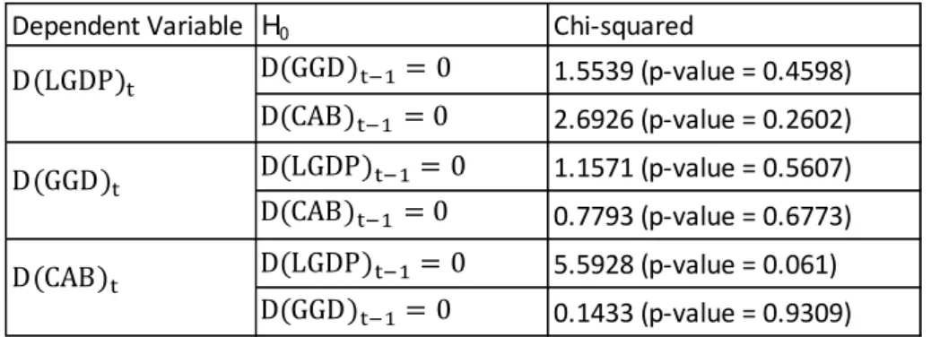
Table 4.9 – Granger causality

Table 4.9 above represents the results from the Granger Causality test. As is can be observed, for every relationship the p-values are above 0.05, which means that we do not have granger causality between the variables, or in other words, no short term relationships exist between the variables.

Dependent Variable H0 Chi-squared

1.5539 (p-value = 0.4598) 2.6926 (p-value = 0.2602) 1.1571 (p-value = 0.5607) 0.7793 (p-value = 0.6773) 5.5928 (p-value = 0.061) 0.1433 (p-value = 0.9309) − = − = − = − = − = − =

(42)

31

4.8. VECM with linear trend

Since many economists seem to agree in the fact that a quadratic trend when choosing the model is not the appropriate way to study cointegration, we opted for following our intuition by choosing the model with linear deterministic trend and intercept. The option to take on this model is explained by the fact that both Trace and Max-Eingenvalue tests being coherent on the number of cointegration vectors.

This model could be defined has:

∆ 𝑡 = 𝜇 + 𝜌 + 𝑝 𝑡 + ′ 𝑡− + 𝜏∆ 𝑡− + ∅ 𝑡+ 𝜀𝑡 (10)

In this model we have ̂ = (− ._.

− . ) and ̂ = ( − .

. )

Which means that in equilibrium we will have the following equation:

𝐿 𝑃𝑡− = + 𝑡𝑟 𝑛 + . 𝑡− − . 𝑡− (11)

Table 4.10 – Cointegration relationship with linear trend model

In contrast with the previous model, although the corresponding alpha being negative for LGDP, the t-statistic is not significant, which means that we should not use LGDP as our dependent variable.

Full results are presented in Annex A8.

Variables Alpha Std. Error t-Statistic D(LGDP) -0.0422 0.03 -1.3954

D(GGD) 1.0877 5.867 0.1854

D(CAB) -8.179 2.503 -3.268

Cointegration vectors =1, observations (n) = 34, Lags = 2. D= 1st differences.

Note: T-value (alpha/std. Error) should be higher then 1.96 in absolute value, in order for the variable to be significant at 5%

(43)

(44)

33

Conclusion

During the years of one of the biggest financial crisis of history, we have observed an uncontrollable accumulation of public debt, which lead to assuming that public debt and GDP may be related. The idea that GDP growth could have been affected by such levels, appeared empirically in 2010. Nowadays, authors assume that the high levels of public debt could be related at some point with slower GDP growth. However, these effects seem to vanish in advanced economies.

During this period, Portugal joined the European Union, adopted the Euro as a new currency and suffered an IMF bailout in the aftermath of the 2008 financial crisis. In this sense, we have used 37 yearly observations, to study the relationship between GDP, public debt and current account balance for the period comprehended between 1980 and 2016 for Portugal.

In order to test the long-term relationship between the variables we have used a VECM model. First, we have tested the stationarity of the variables, showing that all the variables are I (1). Then we used the lag length criteria tests in order to verify the number of lags to include in the model. The result of the test recommended two lags to include in the model. Afterwards the residuals tests proved that we do not have any issue with themselves. We have then used the Johansen cointegration test in order to verify if there is a long-term relationship between the variables, which was proved to exist. Additionally we run Granger causality test, to test for short-run causality. From the results of the test, we conclude that both current account and public debt could not cause GDP in the short-run.

In practical terms, the results of Granger Causality does not mean that Portugal could keep on increasing the public without endangering GDP growth rate since public debt is a burden to the country and the government limiting their political, economic and financial liberty increasing the volatility of the overall system.

After this time-series study further studies need to be developed to try to understand the impacts of public debt, given the fact that Japan, Italy, Greece and Portugal – just to name a few countries – have public debt levels that leave the financial markets nervous about the country’s future capacity to answer shocks.

At the same, variables that can have granger-cause relationship with GDP growth rate are still to be determined on a robust and statistical significance base, which makes us assume that further studies in this discussion will be moving in this direction.

(45)

34

One approach that will probably be repeated in further tests is the economic system panel analysis for granger-cause variables and benchmark of performance metrics, though countries unique systems are difficult to replicate and so a cluster analysis might fall in the trap of comparing incomparable countries.

Summing up, in Portugal, using a time-series approach, even though having a long-term relationship, public debt cannot explain GDP growth rate in the short-run.