Eurasian Journal of Business and Economics 2016, 9 (18), 99-112.
Government Debt Reduction in the USA and
Greece: A Comparative VECM Analysis
Gisele MAH
*, Itumeleng P. MONGALE
**, Janine MUKUDDEM-PETERSEN
***Abstract
The purpose of this paper is to estimate comparative debt reduction models for the USA and Greece using Vector Error Correction Model analysis and Granger causality test. The study provides an empirical framework that could assist in policy formulation for countries with high debt rates as well as those experiencing debt crises. The US model revealed a negative and significant relationship between general government debt and inflation as well as negative significance with primary balance. In Greece, the relationship between general government debts with primary balance is found to be positive and significant while negative and significant with net transfer from abroad. Granger causality is from general government debts to inflation in the USA and from primary balance to general government debts in Greece.
Keywords: Sovereign Debt, Vector Error Correction Model, Granger Causality, Greece, United States of America
JEL Code Classification:H62, H68, H71, C1, C32, C51
UDC:336.276(73+495)
DOI: https://doi.org/10.17015/ejbe.2016.018.06
*
Corresponding author. School of Economics and Decision Sciences, North-West University, South Africa. E-mail: [email protected]
**
University of Limpopo, South Africa. E-mail: [email protected].
1.
Introduction
Sovereign debt reduction has recently proved to be one of the most challenging macroeconomic policies while debt crises are a cause for concern in developed economies (Calitz, 2012). Many developed economies are currently reviewing their fiscal policy with the aim of cutting down rising debt to the ratio of Gross Domestic Product (GDP). In the past, these countries were able to sustain their economies while at the same time, assisting African countries to come out of their debts. It has been observed that sovereign debt crises in advanced economies is constantly on the rise with values more than those stated in the growth and stability path (Mah, Mukuddem-Petersen, Petersen & Hlathwayo, 2013). According to Reinhart and Rogoff (2013), the most popular and significant ways of reducing debt to GDP ratio are through fiscal austerity and restructuring measures, despite the fact that they slow down economic growth. Researchers such as Panizza, Strurzenegger and Zettelmeyer (2013) consider debt default as a measure of reducing rising government debt. On the other hand, Nelson (2013) maintains that governments normally have five major tools they use to address debt. These tools are: fiscal consolidation (spending reduction and/or increase in taxes); debt restructuring (reprogramming of the debt amount); inflation (increase in prices of goods and services); growth (increase in GDP output); and financial repression (increase in interest rates). Despite the fact that there are many ways of cutting down rising government debt, most governments in developed economies are implementing contractionary fiscal policies as a strategy to reduce debt. This phenomenon is widely observed in some economies in America and Europe.
Mencinger, Aristovnik and Verbic (2015) concede that the debate about the connection between economic growth and fiscal policy is still unsettled in academic literature and economic research due its complexity and critical importance. Several studies have been conducted in different parts of the world (such as the European Union, OECD, Latin America and the Caribbean) on the same issue (see Mencinger, Aristovnik & Verbic, 2014); Mencinger, Aristovnik and Verbic (2015); and (Chang, Fabiola & Carballo, 2011). The aim of this study is, therefore, to provide an empirical framework which might assist in policy formulation for countries with high debt rates as well as those experiencing debt crises by undertaking a comparative analysis of government debt reduction strategies in the USA and Greece. This paper will also add to existing literature by providing latest empirical evidence on the impacts of contractionary fiscal policies as well as other measures of reducing government debt.
framework is provided followed by a conclusion and recommendations for stakeholders.
2.
Literature Review
Rising government debt has negative effects on the economy of a country. Public debts are detrimental because they create a burden for future generations since taxes are bound to be raised. Another reason is that a high public debt has a potential to cause the economy to go bankrupt. This is based on S ith’s notion that a government should not get into deficit spending because it is not good for a nation even if the debt is domestic. In particular, Smith postulates that when a government borrows and has to repay the debt, this leads to an increase in taxation, a rise in the flight of domestic capital as well as the devaluation of the currency. Panizza and Presbitero (2012) maintain that sovereign debt seriously reduces the growth of a country towards wealth and prosperity because resources that could have been used by the private sector in a positive way, are transferred to government and used in unproductive activities. It is, therefore, recommended that government should not get into deficits except in cases of emergencies such as wars or natural disasters.
When government finances deficit through taxation, it reduces capital accumulation but not necessarily savings. Taxation may affect investment and the accumulation of new capital, but not the existing productive capital. When a government borrows to finance its deficit, there is a reduction in existing productive capital. Hence, borrowing has more negative effects on the economy as well as the amount of money borrowed by the government and crowds out private investment. This is because borrowed savings which maintains productive labour may be used for unproductive investment (Smith, 1776).
Ricardo (1951) concurs with Smith in the manner in which government spends on unproductive investments as well as the effects of government borrowing. Ricardo is of the opinion that public expenditure that is financed both through taxation and public borrowing, has the same effect. To him, government is expected to redeem its debt in future which can take place in a closed economy through taxation. In a closed economy, when government issues bonds and individuals buy them, that amount is the same as public deficit, hence the interest rate remains the same according to the rational expectation hypothesis. There is no crowding out of private investors and the total demands in the economy remains the same. In an open economy, when public debts are redeemed through sales of assets to international agents (due to inadequate income), government is bound to increase taxes.
maintains that when public debts increase, there is also a corresponding increase in interest rates and falling real wages. Willianson (2008) explains Ricardian Equivalence and the burden of government debt as a burden which must be paid off by taxing citizens in the future. At the individual level, debt represents a liability that redu es a i di idual’s lifeti e ealth. I pra ti e, go er e t a postpo e taxes needed to pay off the debt until long in the future, when the consumers who received the current benefits are either retired or dead.
Most governments borrow large sums of money which causes interest rates to increase. This may discourage private investors from borrowing. When government expenditure increases, aggregate demand also increases. This leads to an increase in income which causes demand for money to increase in the economy. If the supply of money is constant in real terms, interest rates will increase due to an increase in the demand for money. Higher interest rates discourage private investments and aggregate expenditures (Calitz, 2012). Some of the negative effects of government debt are as follows: it affects bond markets, the banking sector and balance of trade; and government debt may lead to an increase in interest rates, decrease in remittances and loss of i estors’ confidence (Mah, Mukuddem-Petersen, Petersen & Hlatshwayo, 2013).
As pointed out by Calitz, government debt causes future generations to pay interest rates and the debt capital while the debt was borrowed to finance the present generation. Debts also increase government expenditures and reduce the amount of money to be invested into productive activities. High government debts may lead to a decline in investor confidence relative to credit worthiness. It also increases interest rates since lenders demand a higher risk premium. Ultimately, higher levels of debt may also affect economic growth (Checherita & Rother, 2012).
Furthermore, Amo-Yartey, Narita, Nicholls, Okwuokei, Peter and Turner-Jones (2012) examined debt dynamics in the Caribbean. They maintain that debt can be reduced by strong growth and lasting fiscal consolidation efforts. They used panel data of 155 countries to analyse determinants of global large debt reduction from 1970 to 2009. Their variables were probability of large debt reduction, real GDP growth, cyclically adjusted primary balance, interest rate payment, debt to GDP ratios and inflation. The results revealed that globally, large debt reduction is caused by decisive lasting fiscal consolidation. Strong economic growth and high debt servicing costs are positively related to the probability of large debt reduction while inflation does not have any effect on debt reduction. The implementation of fiscal consolidation needs to be associated with tax policy and structural reforms.
All these arguments bear testimony to the fact that there is a need to reduce rising government debt which affects many economies.
3.
Research Methodology and Data
The approach by Hosseini
,
Ahmad and Lai (2011) was adopted in this study. These authors used two time series models to compare two countries employing annual time series data from 1970 to 2012. The USA and Greece were selected for this study because even though there are major economic differences between the two economies, the researchers were intrigued by the fact that they have responded differently to high levels of debt. In Greece, the increase in debt led to the implementation of austerity measures as a cure to the crisis while the USA implemented the fiscal cliff. The irony is that Greece seemed to be the most affected of the two economies to a level where it was unable to meet its budget goals. According to The New York Times (2016), the crisis led to a situation where most international banks and foreign investors had to sell their Greek bonds and other holdings. Data used for these models was obtained from various sources. General Government Debt (GDEBT), which is a dependent variable for the two countries, uses data from AMECO. Inflation rate (INF), Primary Balance (PB) and Net Current Transfers from Abroad (RNTRA) are the regressors with data from the World Data Bank. Finally, the fourth regressor of the models, which is the gross domestic product growth (GDPG), uses data from the World Economic Outlook of the IMF.The functional form of the comparative debt reduction model for the two countries is presented as follow:
t t t
t t
t INF GDPG PB RNTRA
GDEBT 01 2 3 4 (2)
and converted into natural logarithm form where equations 3 and 4 represent the debt reduction models for Greece and USA respectively.
(3)
t t t
t t
l
t lUINF lUGDPG lUPB lURNTRA
UGDEBT
l( )0 ( )2 ( )3 ( )4 ( ) (4)
t t t
t t
l
t lGINF lGGDPG lGPB lGRNTRA
GGDEBT
The empirical analysis begins with the unit root tests in order to show the effects of shocks on variables over time. The tests are also worthy in forecasting and in identifying if a regression is spurious (Asteriou & Hall, 2011). The Augmented Dickey-Fuller (ADF), Phillip Perron (PP) and Ng Perron (NP) tests were used in this study in order to obtain a confirmative test of stationarity. Subsequent to that, an appropriate lag length selection was done in order to obtain error terms that are normally distributed, homoscedastic and with no autocorrelation. According to Asteriou and Hall, each of the lag length selection criterion is inspected in order to get the model with the lowest values. In addition, Liew (2004) emphasises that AIC and the FPE lag length results are superior with observations of sixty and below while with observations above sixty, SC and HQ criteria are best in choosing the appropriate lag length.
Cointegration analysis which relies on an error correction model (ECM) was also used in the study such that the dynamic co-movement among variables and the adjustment process towards long-term equilibrium may be examined. In order to achieve this, the Johansen cointegration test with an unrestricted VAR with p-lags of Ytvector and of order q as stipulated by Harris (1995) was employed:
(5)
where represe ts a e tor × , Aiis a × para eters atri a d is an × error term. The advantage of this procedure is that it allows for the possibility of having more than one cointegrating relationship (Chang, Fabiola and Carballo, 2011).
After the cointegration analysis, the Vector Error Correction (VECM) Model was estimated. The model is a good measure of correcting disequilibrium of the previous period which has very good economic implications. It also solves the problem of spurious regression by eliminating trends from the variables when expressed at first difference. Furthermore, the error correction model has an important feature in that disequilibrium error term is a stationary variable. Hence, adjustments processes are involved that prevent the errors in the long run relationship from becoming larger (Asteriou and Hall, 2011). It also involves differencing variables of the study at first difference in an equation while adding a lagged error term to the equation. The VECM model of this study in the form
of variables integrated to the order one is represented as follows:
(6)
where t+1=1, 2, 3, ...T, k stands for the lags number included in the dependent variable ( ). The long run cointegrated coefficient matrix integrated to the order
one is represented as yt1 and the represents the combination of the long run
oi tegrated e tors β and the short run adjustment coefficients
(
)
. The error needs to be negative and statistically significant in order to bring about equilibrium.t p t p t
i
t
A
y
A
y
y
1
...
t
y
tP
O*
k
i
t t i t
t y y
y 1
t
The estimated model was taken through a battery of residual diagnostic and stability tests in order to verify if it met the assumptions of the classical linear regression model. This comprises of the Vector Error Correction (VEC) stability check followed by diagnostic tests such as serial correlation, heteroskedasticity and normality tests.
4.
Empirical Results and Discussion
The results and discussion of all empirical tests of the study are presented in this section. A 5% level of significance is chosen for this study.
4.1
Unit root tests
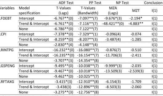
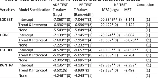
Results for the unit root test for both the USA and Greece are non-stationary at level (see appendices 1 and 2). Since the variables for both countries were found to be non-stationary at level form, there was a need to proceed to first difference. Results for the unit root tests are presented in Tables 1 and 2. The variables are stationary at first difference, that is, at I(1).
The overall conclusion is that all variables under consideration are integrated at the same order, that is, they are I(1) variables. Johansen cointegration analysis was then conducted in order to perform the lag length selection test.
Table 1: Results of ADF, PP and NP tests at first difference for the USA
ADF Test PP Test NP Test Conclusion Variables Modelspecification
T-Values (Lags)
T-Values (Bandwidth)
MZA
(Lags) MZT I(1) LFDEBT Intercept -6.767**(0) -7.097**(7) -9.676*(3) -2.194* I(1) Trend & Intercept -6.761**(0) -7.116**(7) -48.421**(0) -4.883** I(1)
None -6.786**(0) -7.122**(7) I(1)
LCPI Intercept -7.378**(0) -7.329**(1) -0.096(4) -0.074 I(1) Trend & Intercept -8.259**(0) -8.207**(3) -3.487(4) -1.285 I(1)
None -2.830**(4) -4.148**(4) I(1)
LRINTPG Intercept -16.232**(0) -16.080**(7) -0.876(7) -0.510 I(1) Trend & Intercept -16.235**(0) -16.154**(7) -11.706(3) -2.411 I(1)
None -3.707**(3) -14.354**(8) I(1)
LGSPENG Intercept -9.495**(0) -10.038**(7) -9.999*(3) -2.035 I(1) Trend & Intercept -9.467**(0) -10.018**(7) -13.509(3) -2.539(3) I(1)
None -9.462**(0) -10.025**(7) I(1)
LRFTAXG Intercept -3.415*(3) -12.910**(8) -6.154(3) -1.709 I(1) Trend & Intercept -3.438(3) -12.896**(9) -8.503(3) -2.060 I(1)
None -3.275**(3) -12.756**(8) I(1)
Table 2: Results of ADF, PP and NP tests at first difference for Greece
ADF TEST PP TEST NP TEST Conclusion Variables Model Specification T-Values(Lags)
T-Values (Bandwidth)
MZA(Lags) MZT
LGDEBT Intercept -7.068**(0) -7.046**(3) -20.3546**(3) -3.141 I(1) Trend & Intercept -6.996**(0) -6.990**(2) -20.122*(0) -3.122 I(1)
None -5.549**(0) -5.849**(4) I(1)
LGINF Intercept -7.139**(0) -7.145**(1) -20.074**(0) -3.067 I(1) Trend & Intercept -7.603**(0) -7.958**(4) -19.587*(0) -3.070** I(1)
None -7.225**(0) -7.232**(1) I(1)
LGGDPG Intercept -8.528**(0) -9.652**(4) -18.653**(0) -3.053** I(1) Trend & Intercept -5.059**(0) -5.059**(0) -18.838*(1) -2.761 I(1)
None -2.305*8(1) -3.995**(4) I(1)
RGNTRA Intercept -4.135**(0) -4.135**(1) -19.268**(0) -2.358* I(1) Trend & Intercept -3.501(8) -3.939*(1) -18.622*(0) -2.492 I(1)
None -4.246**(0) -4.245**(1) I(1)
* Reject H0: non-stationarity at a 5% level ** Reject H0: non-stationarity at a 1% level
4.2
Lag length selection test
Results of the Lag length selection test are presented in Table 3 and a lag length of 1 was chosen for both countries as suggested by most of the criteria. Furthermore, the Schwarz Information Criterion (SC) was considered due to its effectiveness in many model estimations and also because of its accuracy (Rust, Simester, Brodie and Nilikant, 1995).
Table 3: Selection of the lag length for the USA and Greece
USA
LAG LOGL LR FPE AIC SC HQ Conclusion
0 -228.646 NA 0.082 11.682 11.893 11.758 Not chosen 1 -69.181 271.089* 9.91e-05* 4.959 6.226* 5.417* Chosen 2 -43.338 37.473 0.000 4.917* 7.239 5.757 Not chosen 3 -24.920 22.10175 0.000 5.246001 8.624 6.467 Not chosen
GREECE
LAG LOGL LR FPE AIC SC HQ Conclusion
0 -288.078 NA 1.59134 14.653 14.865 14.730 Not chosen 1 -122.997 280.638* 0.001* 7.649* 8.917* 8.108* Chosen 2 -101.941 30.531 0.002 7.847 10.169 8.687 Not chosen 3 -73.206 34.482 0.002 7.660 11.038 8.882 Not chosen The * indicates the best lag selected by each criterion; sequential modified LR test statistic (LR); Final prediction error (FPE); Akaike information criterion (AIC); Schwarz information criterion (SC); and Hannan-Quinn information criteria (HQ).
4.3
Cointegration tests
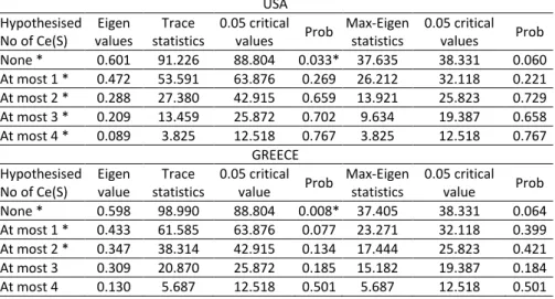
the trace statistics at none, until at most 4, are less than the 5% significance level and greater than the 5% critical value at none, hence the conclusion of one cointegrating equation is drawn. On the other hand, the Max-eigenvalue statistics are less than the 5% critical value at none, up to at most four cointegrating equations, hence the null hypotheses are not rejected and it is concluded that that there is no cointegrating equation. Therefore, the trace test indicates that there is one cointegrating equation while the Max-eigenvalue reveals no cointegrating equation for the US model.
Table 4: Results of Johansen cointegration tests for the USA and Greece
USAHypothesised No of Ce(S)
Eigen values
Trace statistics
0.05 critical values Prob
Max-Eigen statistics
0.05 critical values Prob None * 0.601 91.226 88.804 0.033* 37.635 38.331 0.060 At most 1 * 0.472 53.591 63.876 0.269 26.212 32.118 0.221 At most 2 * 0.288 27.380 42.915 0.659 13.921 25.823 0.729 At most 3 * 0.209 13.459 25.872 0.702 9.634 19.387 0.658 At most 4 * 0.089 3.825 12.518 0.767 3.825 12.518 0.767
GREECE Hypothesised
No of Ce(S)
Eigen value
Trace statistics
0.05 critical value Prob
Max-Eigen statistics
0.05 critical value Prob None * 0.598 98.990 88.804 0.008* 37.405 38.331 0.064 At most 1 * 0.433 61.585 63.876 0.077 23.271 32.118 0.399 At most 2 * 0.347 38.314 42.915 0.134 17.444 25.823 0.421 At most 3 0.309 20.870 25.872 0.185 15.182 19.387 0.184 At most 4 0.130 5.687 12.518 0.501 5.687 12.518 0.501 As far as Greece is concerned, the trace test in Table 4 also shows one cointegrating equation while the Max eigenvalue test indicates zero number of cointegrating equations. If this is the case, it is, therefore, concluded in this study that, there is a long run relationship among variables of the two countries. Lutkepohl,Saikkonen and Trenkler (2000) and Gujarati and Porter (2009) maintain that the trace test is better than the Max-eigenvalue test even though it may be highly distorted in small sample sizes.
4.4
VECM analysis
seems insignificant. It could, therefore, be reasonable for both governments to tolerate relatively higher levels of inflation in order to reduce their level of debts.
Table 5: Results of long-run and short run of VECM for the USA and Greece
Long Run Estimates for USA and GreeceVariables
USA GREECE
Cointergrating equation
Test
statistics Conclusion
Cointergrating equation
Test
statistics Conclusion LUDEBT (-1)
LINF (-1) - 0.312 5.067 (0.061)
Negative,
significant -0.018
0.603 (0.030)
Negative, insignificant LUGDPG (-1) 0.079 -1.689
(0.047)
Positive,
insignificant 0.003
-0.192 (0.015)
Negative and insignificant LUPB (-1) -2.495 7.140
(0.349)
Negative, significant
-0.596 12.020 (0.050)
Positive and significant LRUNTRA(-1) -0.001 0.245
(0.001)
Negative, insignificant
-0.007 3.189 (0.002)
Negative and significant
TREND 0.088 -7.665
(0.011)
Positive & significant
-0.028 3.196 (0.009)
Negative and significant
CONSTANT 72.468 Positive 16.970 Positive
Short Run Estimates for USA and Greece Error
Correction
D
Ludebt Conclusion
D
Lgdebt Conclusion COINTEQ1 -0.021 Negative error term -0.910 Negative error term TEST
STATISTICS
-0.294
(0.071) Insignificant error term
-6.783
(0.134) Significant error term R-SQUARED 0.365
36.5% variation is explained by the independent
variablesin USA
0.630
63% variation is explained by the independent
variables in Greece Standard errors in ( )
For short run estimates, both models show a negative coefficient of the error correction terms which indicates the speed of adjustment to the share of deviation from equilibrium corrected in a single period. A large absolute value of the coefficient equilibrium agents remove a large percentage of disequilibrium in each period, that is, the speed of adjustment is very rapid while low absolute values are indicative of a slow speed of adjustment towards equilibrium. This means in the short run, general government debt in the USA model run at -0.910 (91%) while the Greek model will run at a speed of about -0.021 (2%) to adjust back to equilibrium of the ear’s de iatio .
4.5
Diagnostic tests and stability analysis
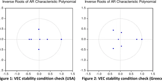
Figures 1 and 2 present results of stability tests in the USA and Greece respectively. Since all the unit roots lie inside the unit of the circle for both models, it is assumed that the estimated models are stable and acceptable in a statistical sense.
-1.5 -1.0 -0.5 0.0 0.5 1.0 1.5
-1.5 -1.0 -0.5 0.0 0.5 1.0 1.5
Inverse Roots of AR Characteristic Polynomial
-1.5 -1.0 -0.5 0.0 0.5 1.0 1.5
-1.5 -1.0 -0.5 0.0 0.5 1.0 1.5
Inverse Roots of AR Characteristic Polynomial
Figure 1: VEC stability condition check (USA) Figure 2: VEC stability condition check (Greece)
5.
Concluding Remarks
relationships established in both countries is in line with empirical studies (such as Bildirici and Ersin, 2007; and Sbrancia, 2011).
Based on the results, it is recommended that the US government should reduce its debt by increasing primary balance (between gross national income and gross national expenditure). The more positive the primary balance is, the more amount of debt likely to be reduced. Similarly, Greece can also reduce its debts by decreasing primary balance and increasing net current transfer since they display a negative relationship.
References
Agnello, L., Castro, V., & Sousa, R. (2013). What determines the duration of fiscal consolidation program? Journal of international Money and Finance, 37, 113-134. https://doi.org/10.1016/j.jimonfin.2013.05.012
Alesina, A. F., & Ardagna, S. (2009). Large changes in fiscal policy: taxes versus spending. NBER working paper.
Amo-Yartey, C., Narita, M., Nicholls, G., Okwuokei, J., Peter, A., & Turner-Jones, T. (2012). The challenges of fiscal consolidation and debt reduction in the Caribbean. Working paper. IMF.
Asteriou, D., & Hall, S. (2011). Applied Econometrics (2nd ed.). New York: Palgrave Maccmillan.
Bildirici, M., & Ersin, O. (2007). Domestic debt, inflation and economic crisis: A panel cointegration application to emerging and developed economies. Applied Econometrics and International Development, 7(1), 33-47.
Calitz, E. (2012). Public debt and debt management. In P. C. Black, Public Economics (4 ed., pp. 323-348). Cape Town, South Africa: Oxford University Press.
Chang, C., Fabiola, C., & Carballo, S. (2011). Energy conservation and sustainable economic growth: The case of Latin America and the Caribbean. Energy policy, 39, 4215-4221. https://doi.org/10.1016/j.enpol.2011.04.035.
Checherita, C., & Rother, P. (2012). The impact of high and growing government debt on economic growth, an empirical investigation for area. European Economic Review Journal, 56, 1392-1405. https://doi.org/10.1016/j.euroecorev.2012.06.007.
Dinca, G., & Dinca, S. (2013). The impact of public debt upon economic growth. International Journal of Education and Research, 1(9).
Gujarati, D., & Porter, C. (2009). Basic Econometrics (5th ed.). Boston: McGraw Hill International Edition.
Heylen, F., Hoebeeck, A., & Buyse, T. (2013). Government efficiency institution and the effects of fiscal consolidation on public debt. European journal of political economy(31), 40-59. https://doi.org/10.1016/j.ejpoleco.2013.03.001.
IMF. (2013). Sovereig de t restru turi g re e t develop e ts a d i pli atio for the fu d’s legal and policy framework. Washington, DC: International Monetary Fund. Retrieved September 2015, from www.imf.org.
Liew, V. (2004). Which lag length selection criteria should we employ? Economics bullentin, 3(33), 1-9.
Lutkepohl, H., Saikkonen, P., & Trenkler, C. (2000). Maximum Eigen value versus trace test for the cointegration rank of a VAR process. Econometrics Journal, 4(2), 287-310. https://doi.org/10.1111/1368-423X.00068.
Mah, G., Mukuddem-Petersen, J., Petersen, M., & Hlatshwayo, L. (2013). Causes, consequence and cures of the Eurozone sovereign debt crisis. In M. Petersen, Economics of debt. New York: Nova Science Publisher.
Me i ger, J., Aristo ik, A., & Ver ič, M. 4 . The i pa t of gro i g pu li de t o
economic growth in the European Union. Amfiteatru Economic, 16(35), 403-414.
Mencinger, J., Aristovnik, A., & Verbic, M. (2015). Revisiting the Role of Public Debt in Economic Growth: the Case of OECD Countries. Inzinerine Ekonomika-Engineering Economics, 26(1), 61–66. https://doi.org/10.5755/j01.ee.26.1.4551.
Mill, J. (1848). Principles of political economy with some of the applications to socail philosophy (7 ed.). London: Longmans, Green and Co.
Nelson, R. (2013). Sovereign debt in Advance Economies: Overview and issues for congress. Congressional Research service. 75 -700.
Panizza, U., & Presbitero, A. F. (2012). Public debt and economic growth: Is there a cause effect. Polis working papers.
Panizza, U., Strurzenegger, & Zettelmeyer. (2013). International government debt. In G. Caprio, The evidence and impact of financail globalisation (pp. 239-254). London: USS: Elsevier.
Reinhart, C., & Rogoff, K. (2013). Financial and sovereign debt crisis: Some lessons learn and those forgotten. 13, 266.
Ricardo, D. (1951). On the Principles of Political Economy and Taxation (Vol. 1817). Cambridge: Cambridge University Press.
Rust, R., Simester, D., Brodie, R., & Nilikant, V. (1995). Model selection criteria: An investigation of relative accuracy, posterior probabilities and combinations of criteria. Management science, 41(2), 322-333. https://doi.org/10.1287/mnsc.41.2.322.
Sbrancia, M. (2011, December 5). Debt and inflation during a period of financial repression. Job Market Paper.
Sheikh, M., Muhammad, Z., & Khadija, T. (2010). Domestic debt and economic growth in Pakistan: An Empirical Analysis. Pakistan journal of Social Science, 30(2), 373-387.
Smith, A. (1776). The wealth of Nations. New York: Random House.
The New York Time. (2016, June 17). Explaining Greece's Debt Crisis. Retrieved June 22, 2016, from www.nytimes.com.
Von Hagen, J., & Strauch, R. (2001). Fiscal consolidation: Quality, economic conditions and sucess. Public Choice, 109, 327-346. https://doi.org/10.1023/A:1013073005104.
Appendices
Appendix 1: ADF, PP and NP tests at level form for the USA
ADF TEST PP TEST NP TEST Conclusion
Variables Model specification
T-Values (Lags)
T-Values (Bandwidth)
MZA
(Lags) MZT
LUDEBT Intercept -0.494(1) 0.263(2) -2.313(1) -0.670 Non stationary Trend & intercept -2.466(1) -1.557(3) -17.584(1) -2.862 Non stationary
None 1.136(1) 1.663(3) Non stationary
LUINF Intercept -2.968*(1) -2.850(2) -11.748*(0) -2.369* Stationary, I(0) Trend & intercept -4.502**(0) -4.299**(5) -18.603*(0) -3.047 Stationary, I(0)
None -1.136(0) -0.976(13) Non stationary
LUGDPG Intercept -5.109**(0) -4.964**(7) 19.884**(0) -3.153 Stationary, I(0) Trend & intercept -5.0771**(0) -4.914**(7) -20.121*(0) -3.167* Stationary, I(0)
None -1.833(1) -2.285*(2) Stationary, I(0)
LUPB Intercept -0.904(0) -0.850(9) 0.909(0) 0.786 Non stationary Trend & intercept -2.461(0) -2.589(2) -10.095(0) -2.217 Non stationary
None 2.507(0) 3.707(9) Non stationary
LRUNTRA Intercept -3.351*(0) -3.259*(2) -12.677*(0) Stationary, I(0) Trend & intercept -4.162*(0) -4.132*(1) -15.057*(0) -2.733 Stationary, I(0)
None -3.384**(0) -3.293**(2) Stationary, I(0)
* Reject H0: non-stationarity at a 5% level ** Reject H0: non-stationarity at a 1% level
Appendix 2. ADF, PP and NP tests at level form for Greece
ADF TEST PP TEST NP TEST Conclusion
Variables Model specification
T-Values (Lags)
T-Values (Bandwidth)
MZA
(LAGS) MZT
LGDEBT Intercept -0.733(0) -0.726708(1) 1.00848(1) 1.04528(1) Non stationary Trend & intercept -1.333(0) -1.296(2) -3.894(0) -1.356(0) Non stationary
None 3.075(1) 3.336(2) Non stationary
LGINF Intercept -1.074(1) -1.117(2) -2.512(1) -0.984 Non stationary Trend & intercept -3.153(0) -3.140(5) -4.837(1) -1.447 Non stationary
None -0.609(1) -0.680(1) Non stationary
LGGDPG Intercept -3.330*(0) -3.299*(0) -13.805*(0) -2.389 Stationary, I(0) Trend & intercept -3.517(0) -3.537*(3) -15.479(0) -2.712 Non stationary
None -3.049**(0) -2.936**(3) Stationary, I(0)
LGPB Intercept -1.651(0) -1.651(0) -0.698(2) -0.381(2) Non stationary Trend & intercept -0.322(0) -0.322(0) -1.760(0) -0.678(0) Non stationary
None -3.721(0) -3.587**(1) Non stationary
LRGNTRA Intercept -1.618(0) -1.688(2) -4.263(0) -1.460 Non stationary Trend & intercept -5.857**(8) -2.025(2) -7.830(0) -1.815 Non stationary
None -1.365(0) -1.380(1) Non stationary