621
Abstract
Geologic modeling is an important step in determining the benefits and final pit dimensions for mining operations. Geostatistical models and distance-based functions are the main methods used to estimate the grade behavior. However, these two meth-ods, despite their similar mean values, differ in spatial variability. The objective of this article is to prove, by comparing the two methodologies, that models with different spatial variability using the Lerchs-Grossmann algorithm will output subtly different final pit dimensions and scheduling. Furthermore, with the direct block schedule (DBS), these differences can be considerable. The tests compared the methodologies using the following three models: inverse distance (ID), ordinary kriging (OK) and turning bands simulation (TBS). The results demonstrate that the Lerchs-Grossmann algorithm is only slightly sensitive to the spatial variability of the grade; however, DBS requires the model populations to be better defined because of its greater sensitivity to spatial variability.
keywords: Mine Planning, Geostatistics, Geologic Modeling, Direct Block Scheduling,
Lerchs-Grossmann. Luiz Alberto Carvalho1
Felipe Ribeiro Souza2
Leonardo Soares Chaves3
Beck Nader4
Taís Renata Câmara5
Vidal Félix Navarro Torres6
Roberto Galery7
1Mestre em Tecnologia Mineral, Universidade
Federal de Minas Gerais - UFMG, Escola de Engenharia, Programa de Pós-Graduação em Engenharia Metalúrgica, Materiais e de Minas, Belo Horizonte – Minas Gerais – Brasil.
2Professor-Assistente, Universidade Federal do
Mato Grosso - UFMT, Instituto de Engenharia, Várzea Grande - Mato Grosso - Brasil. [email protected]
3Pesquisador, Instituto Tecnológico Vale,
Ouro Preto – Minas Gerais - Brasil. [email protected]
4Professor-Doutor, Universidade Federal de Minas
Gerais - UFMG, Escola de Engenharia, Departamento de Engenharia de Minas, Belo Horizonte – Minas Gerais – Brasil. [email protected]
5Pesquisadora, Instituto Tecnológico Vale,
Ouro Preto – Minas Gerais - Brasil. [email protected]
6Pesquisador, Instituto Tecnológico Vale,
Ouro Preto – Minas Gerais - Brasil. [email protected]
7Professor-Titular, Universidade Federal de Minas
Gerais - UFMG, Escola de Engenharia, Departamento de Engenharia de Minas, Belo Horizonte – Minas Gerais – Brasil. [email protected]
Impact of grade distribution
on the final pit limit definition
http://dx.doi.org/10.1590/0370-44672017710150
1. Introduction
Determining the lithology and grade distribution in a deposit is highly relevant to the mineral industry. The spatial distri-bution of the samples directly influences the estimation of resources and reserves (NERY, 1995). The reliability of the geo-logical spatial distribution, its shape and grade distribution have important effects on later stages of a project. However, when a geostatistical approach is applied, the following typical problems can occur (JOURNEL and HUIJBREGTS, 1989):
- Global and local estimation: esti-mation methods that have local accuracy, usually employing interpolation methods, produce results that “smooth” the values, causing a variation of the phenomena as a whole. In contrast, global methods, usually involving simulations, have the opposite effect, resulting in good overall definition with a loss of local accuracy (FURUIE, 2009).
- Supporting effect: the estimation process is completed by generating blocks with grade distribution, with separate es-timations for each block of the model. The definition of the block dimensions has a great influence on the estimation since the definition is performed based on informa-tion obtained by drill holes with much smaller dimensions than the estimated block. This situation requires the definition of the best block dimension to ensure the reliability of the resource estimation for the data (NERY, 1995).
- Data distribution: it is common to have clustered data in space, either due to intentional choice or to an unavoidable need at the moment the sample is obtained. These clustered data cause a bias in the resource estimation because the data do not accurately represent the study region. To overcome this problem, there are several ungrouping methods, such as influence polygons, moving windows, mean kriging, etc. (CORNETTI, 2003; SOUZA, WEISS,
et al., 2001).
These problems can lead to mine planning errors, such as differences be-tween the estimated and actual data, larger block estimates for actual drilling blocks that exceed equipment capacity, and increased mining costs due to as-sumptions of different rock types than are actually present. It should be noted that the estimation methods are not free of errors due to the existing fundamental errors in the various steps that make up the entire process (GRIGORIEFF, COSTA and KOPPE, 2002); however, the method attempts to minimize errors. Generally, homogeneous deposits present good results for interpolation methods, such as kriging and inverse distance (ID). Simulations are used to circumvent the smoothing problem and provide variability of the deposit that may be more representative of reality than the values estimated with another method (JOURNEL and HUIJBREGTS, 1989). However, these simulations are not error free (OLEA, 1999) and do not provide a representative scenario but, rather, a set of equally likely scenarios.
The ID method is a very popular spatial interpolation method based on the premise that the points in any pair of points have a relationship with each other; this re-lationship is inversely related to the distance between their positions (LU and WONG, 2008). Kriging is the general name given to linear regression techniques that minimize the variance of estimates, variances that were defined in an earlier experimental semivariogram model (OLEA, 1991). Geo-statistical simulation techniques attempt to generate several simulated scenarios based on an algorithm and do not present the smoothing data problem; therefore, the use of this technique is one possible way to avoid the existing problem in kriging. The turning band simulation (TBS) method simplifies the multidimensional space prob-lem using one-dimensional simulations and extends them to 2D or 3D space (AFZAL,
ALHOSEINI, et al., 2014).
The classical methodology for final pit definition applies the Lerchs-Gross-mann (LG) algorithm “to draw the contour of an open pit in a way to maximize the differences between the total value of the exploited mineralization and the total cost of mining the ore and waste” (LERCHS and GROSSMANN, 1965). The result of the algorithm is an optimum final pit; how-ever, it does not consider the time required for the extraction of each block, which is necessary to divide the pit into phases and, in a later stage, conduct production plan-ning (GOYCOOLEA, MORENO and RIVERA, 2013). Direct block scheduling (DBS) has evolved (JÉLVEZ, MORALES,
et al., 2016), enabling the algorithms to
work by generating pits under various physical and operational constraints. The major difference is the consideration of the extraction time to determine the values of the blocks, which is more representa-tive of reality, mainly due to the attempt to perform a determination of the pit considering operational constraints that commonly occur but are not considered in LG, such as stockpiling and multiple destination possibilities.
In industry, spatial variability does not receive proper attention; instead, the average values are considered, especially for the grade values. During mine planning, mining higher-graded regions can antici-pate revenues and increase the net present value (NPV) of a project. This is one of the bases of DBS, which considers the period of each block extraction to calculate the expected income.
Existing methods for generating the geological model and the pit make clear the relevance of studying the combination between these methods and their different results to determine the best combination between model generation and pit deter-mination techniques that will produce the minimum error to meet user objectives.
Literature review
Spatial estimates were typically per-formed via the ID technique, in which weights are assigned to the samples as an inverse function of the distances between the samples and the points to be estimated. The power number (p) can assume any in-teger value, most commonly 2 (BABAK and DEUTSCH, 2009). However, this method has great limitations (SRIVASTAVA, 2013); for example, it does not allow the variation
of weights based in other information, it does not consider the possibility of redun-dant samples, it generates errors due to the division by zero when the distance is zero, and it does not provide a mechanism to evaluate the reliability of the results.
Currently, estimates are made mostly via the kriging (RAVÉ, JÍMENEZ-HOME-RO, et al., 2014) method, which provides
effective solutions compared to the
623 easily satisfied assumptions, simple data
requirements and variogram implementation function (OLIVER and WEBSTER, 2014). The variogram is a theoretical function of the random study process obtained by an analysis of the data values for different distances in a certain direction. With the variogram function, kriging solves a set of linear equations, known as the kriging system, which contains semivariants of the function.
The TBS method is a stochastic spa-tial simulation that uses a nonlinear data transformation for the Gaussian domain (MATHERON, 1973). The method is con-sidered an approximative algorithm due to its random runs, in which the distributions are close to the multivariate Gaussian distri-bution of the input data, since the simulated fields are non-ergodic (FURUIE, 2009). This methodology works with a reduction in the dimensional space; in other words, it uses data in two or three dimensions, simpli-fies them to a one-dimensional space and
performs several independent simulations (FURUIE, 2009).
The optimal final pit definition is typically defined based on the block value of the geological input model. The LG algorithm is mathematically based on the representation of the problem by graphs G = (V, A), defined as a collection of the set V of elements Vj (j = 1, 2,..., n) called nodes of G, with a set A of pairs of elements of x, called arcs or branches of the graphs. Each block corresponds to a node and receives a “weight” that is its value. The algorithm then constructs a graph from the base of the operation, defining “strong” and “weak” branches. The branches are created from the bottom of the pit to the surface, defining the optimal contour of the pit. The pit contains the highest possible sum of block “values,” respecting the constraints such as general slope stability and blocks of precedence (CARMOS, CURI and SOUSA, 2006). The major issue with the algorithm is that it does not consider time when assigning the block
values; therefore, the generated optimum pit is an optimum instant pit. After the final pit is defined by the LG algorithm, it is neces-sary to determine the production sequence, called pushbacks, to determine the sequence of mining according to the operational ca-pabilities of the project.
The DBS algorithm attempts to over-come the main LG issue, and it generates the most valuable pit considering the time of extraction for each block, its various desti-nation possibilities and the production con-straints. The greatest difficulty with these new methods is the need to use heuristics to achieve a solution, which does not guarantee an optimal final result (RAMAZAN, 2006). Techniques such as a tabu search, Lagrange decomposition and fundamental tree are used as tools for the development of these algorithms. Generally, all techniques are based on the same principle to maximize the project net present value subject to restric-tions that may vary according to the project requirements and the intent of its creators.
2. Methodology
Resource estimation
A database of drill holes from an iron ore mine was used in this study. The mine is located in the iron
quadrilateral region in the state of Minas Gerais. The database contains geo-referenced information from drill
holes, and a summary of the random variable iron grades is provided in Table 1.
Variable Minimum (%) Maximum (%) Mean (%) Standard deviation (%)
Iron 5.40 62.62 45.72 11.72
Table 1 Summary of iron samples.
To conduct the study of the reserve, three resource models were created. The first model was obtained with the ID technique with a power value of 2. The second model applied OK with search
ellipsoids with the parameters obtained from the semivariogram analysis. The third model was based on 25 simulations using the TBS method with data from the search ellipsoid. For all models, a
minimum of 4 samples and a maximum of 12 were chosen for the estimation of each block. The block size was chosen based on operational factors and the experience of researchers from similar projects.
Resources modeled by kriging
The data were analyzed and validat-ed using SGeMs (Stanford Geostatistical Modeling Software). It was necessary to
decluster the data to obtain the experi-mental semivariogram. Figure 1 shows the optimized result of the declustering
process with the values at 1280 meters in the X- and Y-directions as well as 18.5 meters in the Z-direction.
The declustered data were used to determine the experimental variograms used to build the theoretical model. The
main direction determined was N40°, and the secondary direction was the per-pendicular direction (D-90). A summary
related to the variography stage is shown in Table 2 and Figure 2. The best fit was based on the spherical model.
Adjustment data Value
Range X 600 m
Range Y 450 m
Range Z 130 m
Sill 80
Nugget Effect 15
Table 2
Search ellipsoid data for ordinary kriging and inverse distance method.
Figure 2
Adjustment variogram for N40° according to the spherical model.
Resources modeled by inverse distance
The construction of the model based on the ID used the same parameters for the
search ellipsoid as in the kriging modeling (Table 2). A power value of 2 was used in the
estimation, which is based on the deposit stratification and smooth grade transition.
Resources modeled by turning bands simulation
The data and spatial analysis deter-mined with the kriging method were used on the TBS. For this simulation, a
Gauss-ian transformation of the grade data was necessary (Figure 3). The variogram with normalized iron grades is shown in Figure
4, and the variographic parameters were reanalyzed to determine the new search neighborhood (Table 3).
Figure 3
Histogram of Fe Gaussian grades.
Figure 4
Adjusted variogram of
625
Adjustment data Value
Range X 650 m
Range Y 380 m
Range Z 150 m
Sill 0.55
Nugget Effect 0.22
Table 3 Search ellipsoid data for turning bands simulation.
Model 1st component 2nd component Global
Mean (%) Std. Dev. (%) Mean (%) Std. Dev. (%) Mean (%) Std. Dev. (%)
ID 40.0 4.0 58.0 6.0 44.84 8.85
OK 39.0 6.0 59.0 3.5 44.53 10.45
TBS 44.0 7.0 64.0 5.0 44.18 10.57
Table 4 Mean and standard deviation of the generated models.
Figure 5 Block models from ID, OK and TBS.
Production sequencing
As reported in the resource estima-tion topic, 3 block models were developed according to different methods. The ID, OK and TBS methodologies resulted in models with different means (Table 4), variability and spatial distribution (Figure 5). Accord-ing to (GOYCOOLEA, MORENO and RIVERA, 2013), DBS is more sensitive to changes in the benefit function; in the pres-ent study, to change the benefit function,
different grades were used from the three models. To define the benefit function, it is necessary to calculate the likely revenue and mining cost of each block. The benefit func-tion model used is represented in Equafunc-tions (1), (2) and (3).
(1) Benefit Function = Block Value – Block Costs
(2) Block Value = Recovered Material x Price
(3) Block Cost = Mined Material x Sum of Costs per Block.
For the pit definition by LG and DBS, the input parameters of Tables 5 and 6 were used. The final pit limit study for the LG methodology was conducted using the Mi-cromine software , while the scheduling was done using Whittle software choosing the best case situation for pushbacks, and DBS was performed using the Simsched software.
Parameter Value
Dilution 0%
Mine recovery 100%
Sales Price 55 US$
Mine Cost (Ore and Waste) 2.59 US$/t
Administrative Cost 0.63 US$/t
Process Cost 5.85 US$/t
Sales Cost 10.13 US$/t (Product)
Cut-Off Rich Ore 52%
Cut-Off Poor Ore 30%
Production Target 200 Mt ROM/Year
Discount Factor 10%/Year
Parameter Value
Vertical Advance 40 m
Horizontal Advance 70 m
Operational Base 50 m
Pit Base 50 m
Strip Ratio None
Grade Control None
Slope Angle 40º Table 6
Operational input data for DBS and LG.
3. Results and discussion
The models generated in the pre-vious section were used to delineate the final pit and for production sequenc-ing. The LG method was applied only for the ID and OK models since it is not possible to use simulated block models in the classical methodology.
For the DBS, it was possible to use all three models. A statistical sum-mary of the grade distribution of these models is provided in Table 4. These results illustrate that all the models presented two distribution families called components and that the
aver-age grade of the simulations presented an overestimation of the data when compared to the models generated by the two other methods. The different models presented different results for grade, NPV and the period in which the blocks should be mined.
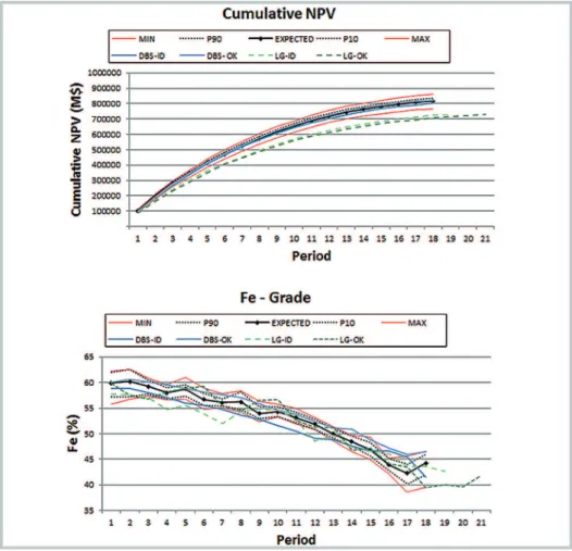
Figure 6
Results of cumulative NPV and Fe grade tests.
Figure 6 shows that the difference between the grade curves reached by DBS is almost constant, and the grade level of OK is higher. The same figure indicates that the grade curve that represents se-quencing by the LG method oscillates more for the two models. According to Table 4, the OK scenario presents a greater global standard deviation than the ID model, but the spatial variability of the model was not considered as a decisive
fac-tor for the variability of planning grades. The fact that the standard deviation dif-ference was small did not decisively cause intense iron grade fluctuations. However, the two deposits presented intense oscilla-tion when submitted to the LG methodol-ogy. The ID in both cases (LG and DBS) remained below the P10 curve. The P10 curve represents the 10% probability that the scenario would occur when compared to the simulated model. Consequently, it
can be concluded that the ID generated a low realization probability scenario during mining operations, even when the average and standard deviations were close to those of other models.
627 population of 60% is more voluminous in
order to increase both the mean planning grades. In both methodologies, the OK
model generated a mining plan closer to the most likely scenario. DBS is able to analyze each block individually; therefore,
it was able to select blocks with higher grades in earlier periods in comparison with LG.
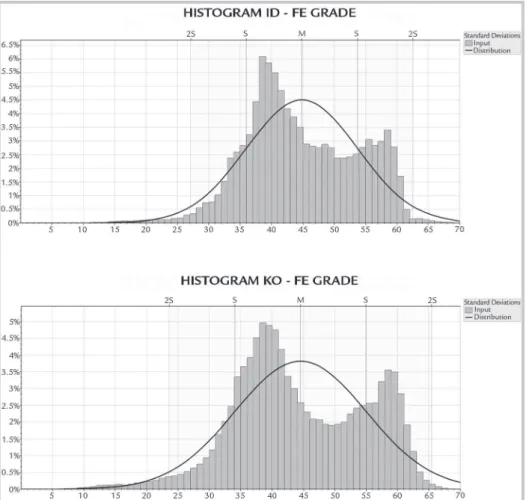
Figure 7 Histograms of block models (ID and OK).
The higher initial grades reached by the DBS made it possible to achieve higher NPV with this methodology,
even when the higher-graded blocks were not grouped in the same region. Achieving selectivity or richer blocks
in the initial periods is more difficult for the LG algorithm according to (SOUZA, 2016).
Comparison Percentage of blocks mined in different periods (%)
ID - SDB x TBS - SDB 19.05
OK - SDB x TBS - SDB 15.09
ID - LG x TBS - SDB 27.95
OK - LG x TBS - SDB 27.90
Table 7 Comparison between mining block periods of different models.
After the different methodologies were verified to have generated different results according to the standard grade deviation, Table 7 was constructed. This table counts the number of mined blocks in different periods other than the simulated scenario. The simulated
scenario was adopted as a reference considering the different probabilities of geological grades. The results show that, as shown in Figure 6, the differ-ence between ore populations does not dramatically affect the LG methodology; therefore, the blocks mined by ID and
OK are almost the same in comparison to the simulated model. However, the better defined populations made DBS for the OK model more consistent with the simulated models. Thus, the better defined the populations in the block models, the more accurate the DBS.
4. Conclusion
The methods for generating a geo-logical model differ considerably, includ-ing differences in their mathematical basis and execution. The present study evaluated the impacts caused by different methods for obtaining the block model on mine planning steps by employing
the deterministic method via LG and stochastic simulation in DBS. The results show that with the classical methodology, a difference up to 27.95% exists in mine scheduling regarding the timing of when different blocks should be mined. In the classical deterministic method (LG) the
OK model, whose populations are better delimited, presented lower grade fluctua-tions. Due to the greater block selectivity, DBS presented a higher average grade. The model based on the ID method generated an average grade close to P10, which is a low-probability scenario that likely underestimates the reserve potential. The
LG methodology was revealed to be less sensitive to the block population variabil-ity, justifying a common practice in mine planning and comparing models only by mean grades. In LG, there is no intense selectivity of these different populations. Using DBS, it is necessary to analyze the individual populations because changes
in spatial distribution have great influence on mine scheduling. Deposits with well-defined and numerous populations tend to present higher NPV results under the DBS methodology. The greater the variability and number of different populations in a deposit, the farther the response of the LG methodology is from the likely scenario.
Acknowledgments
The authors would like to thank the Programa de Pós-Graduação em Engenharia Metalúrgica, Materiais e de Minas (PPGEM), Coordenação
de Aperfeiçoamento de Pessoal de Nível Superior - Programa de excelência acadêmica (CAPES-PROEX), Conselho Nacional de Desenvolvimento
Cientí-fico e Tecnológico (CNPq), Fundação de Amparo à Pesquisa do Estado de Minas Gerais (FAPEMIG) and Instituto Tecnológico Vale (ITV).
References
AFZAL, P. et al. Outlining of high quality coking coal by concentration–volume frac-tal model and turning bands simulation in East-Parvadeh coal deposit, Central Iran. International Journal of Coal Geology, p.88-99, 2014.
BABAK, O., DEUTSCH, C. V. Statistical approach to inverse distance interpolation.
Stochastic Environmental Research and Risk Assessment, p.543-553, 2009.
CARMOS, F. A. R., CURI, A., SOUSA, W. T. D. Otimização econômica de explota-ções a céu aberto. Revista Escola de Minas, Ouro Preto, p.317-321, 2006.
CORNETTI, M. A. O impacto do uso de ponderadores de dados agrupados na Geoestatística. Campinas: Universidade Estadual de Campinas, 2003. p.99.
(Masters Dissertation).
FURUIE, R. D. A. Estudo comparativo de métodos geoestatísticos de estimativas e simulações estocásticas. São Paulo: Universidade Federal de São Paulo, 2009.
p.183. (Masters Dissertation).
GOYCOOLEA, M., MORENO, E., RIVERA, O. Direct optimization of an open cut Scheduling Policy. Proceedings of APCOM, p.424-432, 2013.
GRIGORIEFF, A., COSTA, J. F. C. L., KOPPE, J. O problema de amostragem manual na indústria mineral. Revista Escola de Minas, Ouro Preto, v. 55, n.3.
p. 229-233, 2002.
JÉLVEZ, E. et al. Aggregation heuristic for the open-pit block scheduling problem.
European Journal of Operational Research, p.1169-1177, 2016.
JOURNEL, A. G., HUIJBREGTS, C. J. Mining geostatistics. San Diego: Academic
Press , 1989.
LERCHS, H., GROSSMANN, L. F. Optimum design of open-pit mines. Canadian Mining and Metallurgical Bulletin, Montreal, p.17-24, 1965.
LU, G. Y., WONG, D. W. An adaptive inverse-distance weighting spatial. Computers & Geosciences, p.1044-1055, 2008.
MATHERON, G. Principles of geostatistics. Economic Geology, p.1246-1266, 1963.
MATHERON, G. Les variables régionalisées et leur estimation. Paris: Masson,
1965. p. 305. (Monograph).
MATHERON, G. The intrinsic random functions and their aplications. Advances in applied Probability, p.439-468, 1973.
NERY, M. A. C. O problema da estimativa de recursos minerais no estudo da exiquibilidade de lavra. Campinas: Universidade Estadual de Campinas, 1995.
p. 113. (Masters Dissertation).
OLEA, R. Geostatistical glossary and multilingual dictionary. [S.l.]: Oxford
University Press, 1991.
OLEA, R. A. Geostatistics for engineers and earth scientists. [S.l.]: Kluwer Academic
Publishers, 1999.
OLIVER, M. A., WEBSTER, R. A tutorial guide to geostatistics: computing and mo-delling variograms and kriging. Catena, p.56-69, 2014.
RAMAZAN, S. The new fundamental tree algorithm for production scheduling of open pit mines. European Journal of Operational Research, p.1153-1166, 2006.
629 Received: 19 October 2017 - Accepted: 19 February 2018.
(GPGPU) to accelerate the ordinary kriging algorithm. Computers & Geosciences,
Tarrytown, v. 64, p. 1-6, 2014.
SOUZA, F. Sequenciamento direto de blocos: impactos. limitações e beneficios para aderência ao planejamento de lavra. Belo Horizonte: Universidade Federal de
Minas Gerais, 2016. (Masters Dissertation).
SOUZA, L. E. et al. Impacto do agrupamento preferencial de amostras na inferência estatística: aplicações em mineração. Revista Escola de Minas, Ouro Preto, v. 54,
n.4, p.257-266, 2001.
SRIVASTAVA, M. Geostatistics: a toolkit for data analysis, spatial prediction and risk ma-nagement in the coal industry. International Journal of Coal Geology, p. 2-13, 2013.