Integration in the Brazilian telecommunication industry:
The case of Vivo and TIM
Filipe Barros
152112308
June 2014
Advisor: Peter Tsvetkov
Programme:
Master of Science in Business Administration
Major in Corporate Finance
Abstract
The telecommunications sector in Brazil has been facing a particular attention from international groups during the last decade. All four main players in Brazil are controlled by global telecom players and several strategic moves have taken place during the past few years in Latin America. This is the case of Telefónica ownership in Vivo, Telecom Italia participation in TIM, the recent merger between Oi and Portugal Telecom, among several asset divestures throughout Latin America countries from both Telefónica and Telecom Italia.
Many analysts and investment bankers have suggested that a possible sell of TIM from Telecom Italia is likely to occur due to high leverage ratios from the parent company. The company has divested in several Latin American and European operations in order to reduce debt, but, the leverage continues to increase.
We foresee that an acquisition of TIM by Vivo would completely change the industry in Brazil and that the overlap between both players would create synergies above the value of TIM. We forecast a standalone valuation for Vivo and TIM of BRL 56.2 Billion and BRL 26.5 Billion, respectively, and a merged firm enterprise value of BRL 113.8 Billion, corresponding to an expected synergies amount of nearly BRL 31.2 Billion.
Nevertheless, the Brazilian regulator could impose several restrictions to the merger, since the combined firm would have market shares above 70% in several states, and, as a result, we expect that an asset by asset sale would be the most appropriate scenario in reality.
The case of Vivo and TIM II
Acknowledgements
The author would like to thank Professor Peter Tsvetkov for the guidance and availability during the development of the thesis; to Pedro Palos, Miguel Salgado and Daniel Pimentel for the insightful knowledge on Telecoms and data provided; to Francisco Valério for being my 3rd floor buddy, with whom I had numerous discussions on methodologies and critical issues and, in general, to all my friends and family for the constant motivation and support.
I
NDEX
0. INTRODUCTION ... 1 1. LITERATURE REVIEW ... 2 1.1. COST OF CAPITAL ... 2 1.1.1. CAPM ... 2 1.1.2. Risk-Free rate ... 3 1.1.3. Beta ... 31.1.4. Market risk premium ... 5
1.1.5. Cost of debt ... 6
1.1.6. WACC ... 6
1.2. VALUATION METHODS ... 8
1.2.1. Note on Free Cash Flow method ... 8
1.2.2. Discounted Cash Flow method using WACC ... 8
1.2.3. Adjusted Present Value ... 9
1.2.3.1.Free Cash Flow valuation at unlevered cost of equity ... 10
1.2.3.2.Leverage side effects valuation ... 10
1.2.4. Multiples valuation ... 11
1.3. VALUATION IN EMERGING MARKETS ... 13
1.3.1. Why is emerging market valuation so important? ... 13
1.3.2. Proposed solutions ... 13
1.4. MERGERS AND ACQUISITIONS ... 15
1.4.1. Why M&A happens? ... 15
1.4.2. Why is cross-border M&A important? ... 15
1.4.3. Does M&A pay? ... 16
1.4.4. Payment methods ... 16
1.4.5. How to avoid the synergy trap ... 17
2. INDUSTRY REVIEW AND MARKET ASSESSMENT ... 19
2.1. GLOBAL TELECOM TRENDS ... 19
2.2. DATA TRENDS ... 21
2.3. TELECOM OPERATORS TRENDS... 23
2.4. ECONOMICS AND DEMOGRAPHICS OF BRAZIL ... 25
2.5. THE TELECOMMUNICATIONS SECTOR IN BRAZIL ... 26
2.6. VIVO COMPANY REVIEW ... 29
2.6.1. Revenues ... 29 2.6.2. Costs ... 30 2.6.3. Capital expenditures ... 30 2.6.4. Net Debt ... 31 2.7. TIMREVIEW ... 32 2.7.1. Revenues ... 32 2.7.2. Costs ... 33 2.7.3. Capital Expenditures ... 34
The case of Vivo and TIM IV
2.7.4. Net Debt ... 35
2.8. REVENUE AND COST DRIVERS ... 36
2.8.1. Revenue Drivers ... 36 2.8.2. Cost Drivers ... 37 3. VIVO VALUATION ... 39 3.1. INTRODUCTION ... 39 3.2. FCFF PROJECTIONS ... 39 3.2.1. Revenues ... 39 3.2.1.1.Mobile revenues ... 40
3.2.1.2.Fixed and handset revenues ... 41
3.2.2. Costs ... 43
3.2.3. Depreciations, amortizations and CAPEX ... 44
3.2.4. Working capital ... 45
3.2.5. Debt and interest tax shields ... 46
3.3. VIVO VALUATION USING THE APV APPROACH ... 47
3.4. SENSITIVITY ANALYSIS ... 49
3.4.1. Bull-Bear scenarios ... 49
3.4.2. Sensitivity to individual variables ... 50
3.4.3. Sensitivity to the discount rate and growth rate ... 50
3.5. RELATIVE VALUATION ... 51 3.6. CONCLUSIONS ... 52 4. TIM VALUATION ... 53 4.1. INTRODUCTION ... 53 4.2. FCFF PROJECTIONS ... 53 4.2.1. Revenues ... 53 4.2.2. Costs ... 55
4.2.3. Depreciations, amortizations and CAPEX ... 56
4.2.4. Working Capital ... 57
4.3. TIM VALUATION USING DISCOUNTED CASH FLOW APPROACH WITH WACC ... 58
4.4. SENSITIVITY ANALYSIS ... 59
4.4.1. Bull-Bear scenarios ... 59
4.4.2. Sensitivity to individual variables ... 60
4.4.3. Sensitivity to the discount rate and growth rate ... 61
4.5. RELATIVE VALUATION ... 61
4.6. CONCLUSIONS ... 62
5. PARENT COMPANIES REVIEW ... 63
5.1. TELECOM ITALIA ... 63
5.2. TELEFÓNICA ... 65
6. THE SYNERGIES ANALYSIS ... 68
6.2. SYNERGIES ANALYSIS ... 71
6.2.1. Cost synergies ... 71
6.2.2. Revenue synergies ... 74
6.2.3. CAPEX synergies ... 75
6.2.4. Incremental cash flows with merger ... 76
6.2.4.1.Incremental gains ... 76
6.2.4.2.Incremental expenses ... 76
6.2.5. Synergies summary... 77
6.2.6. Synergies split analysis ... 79
7. THE MERGED COMPANY AND THE DEAL ... 80
7.1. THE FINANCIALS WITH SYNERGIES ... 80
7.1.1. Revenue ... 80
7.1.2. Costs and EBITDA ... 80
7.1.3. Depreciations and Amortizations ... 82
7.1.4. EBIT ... 82
7.2. THE DEAL ... 84
7.2.1. Structure of the acquisition ... 84
7.2.2. Discount rate ... 86
7.2.3. Merged Firm Valuation ... 87
7.2.4. Synergies valuation and shareholder’s gain ... 89
7.2.5. Value created and “Meet the premium line” ... 91
7.2.6. Sensitivity analysis ... 92
7.2.6.1.Bull-Bear scenarios ... 92
7.2.6.1. Sensitivity to Premium, Stock issuance and discount rate ... 93
7.2.7. Regulatory constraints ... 95
8. CONCLUSIONS ... 98
APPENDIX ... 99
The case of Vivo and TIM VI
I
NDEX OF
F
IGURES
FIGURE 1–MOST WIDELY USED VALUATION METHODS ... 12
FIGURE 2–ACQUISITION VALUATION FRAMEWORK ... 17
FIGURE 3–MEET THE PREMIUM LINE ... 18
FIGURE 4–CORRELATION BETWEEN GDP PER CAPITAL AND PENETRATION ... 19
FIGURE 5–MOBILE SUBSCRIBERS PER CONTINENT... 20
FIGURE 6-GLOBAL BROADBAND EVOLUTION ... 21
FIGURE 7–GLOBAL DATA CONSUMPTION ... 21
FIGURE 8–NEW DIGITAL PARADIGM ... 22
FIGURE 9–A BUSINESS MODEL FOR TELECOM OPERATORS ... 23
FIGURE 10–NEW CHALLENGES FOR TELECOM OPERATORS ... 24
FIGURE 11–DEMOGRAPHICS OF BRAZIL ... 25
FIGURE 12–BRAZILIAN GDP EVOLUTION ... 25
FIGURE 13–MOBILE,3GCONNECTIONS AND BRAZILIAN MOBILE PENETRATION ... 26
FIGURE 14-MARKET SHARE PER OPERATOR ... 27
FIGURE 15–AVERAGE REVENUE PER USER PER OPERATOR ... 27
FIGURE 16–FIXED CONNECTIONS AND INTERNET USERS... 28
FIGURE 17-VIVO REVENUES PER PRODUCT ... 30
FIGURE 18–COST ANALYSIS ... 30
FIGURE 19-VIVO CAPITAL EXPENDITURES ... 31
FIGURE 20-VIVO NET DEBT ANALYSIS ... 31
FIGURE 21–TIMREVENUES PER PRODUCT ... 33
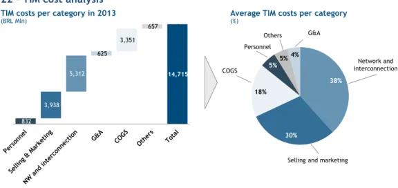
FIGURE 22–TIM COST ANALYSIS ... 34
FIGURE 23–TIM CAPITAL EXPENDITURES ... 35
FIGURE 24–TIM NET DEBT ANALYSIS ... 36
FIGURE 25–NUMBER OF SUBSCRIBERS PER EMPLOYEE PER COUNTRY ... 38
FIGURE 26–VIVO STOCK PRICE EVOLUTION ... 39
FIGURE 27–VIVO REVENUES PER CATEGORY ... 40
FIGURE 28–VIVO MOBILE REVENUE DRIVERS ... 41
FIGURE 29–VIVO MOBILE REVENUES FORECAST ... 41
FIGURE 30–VIVO FIXED AND HANDSET REVENUE DRIVERS ... 42
FIGURE 31–VIVO FIXED AND HANDSET REVENUES ... 43
FIGURE 32–VIVO COSTS DRIVERS ... 44
FIGURE 33–VIVO OPERATIONAL COSTS ... 44
FIGURE 34–VIVO D&A AND CAPEX FORECAST ... 45
FIGURE 35–VIVO WORKING CAPITAL ... 46
FIGURE 36–VIVO BEAR –BULL SCENARIOS ... 49
FIGURE 37–VIVO INDIVIDUAL SENSITIVITY ANALYSIS ... 50
FIGURE 38-VIVO MULTIPLE ANALYSES ... 51
FIGURE 39–VIVO ENTERPRISE VALUE COMPARISON ... 52
FIGURE 40–TIM STOCK PRICE EVOLUTION ... 53
FIGURE 41–TIMREVENUE DRIVERS ... 54
FIGURE 43–TIM COST DRIVERS ... 56
FIGURE 44–TIM OPERATIONAL COSTS ... 56
FIGURE 45–TIMD&A AND CAPEX FORECASTS ... 57
FIGURE 46–TIM WORKING CAPITAL ... 57
FIGURE 47–TIM CAPITAL STRUCTURE AND COST OF CAPITAL ... 59
FIGURE 48-BEAR –BULL SCENARIOS ... 60
FIGURE 49-TIM INDIVIDUAL SENSITIVITY ANALYSIS TO THE ENTERPRISE VALUE ... 60
FIGURE 50-TIM MULTIPLE ANALYSIS ... 62
FIGURE 51–TIM ENTERPRISE VALUE COMPARISON ... 62
FIGURE 52–TELECOM ITALIA STOCK COMPARISON WITH FTSEMIB AND S&P500 ... 63
FIGURE 53-TELECOM ITALIA REVENUES AND EBITDA MARGIN ... 64
FIGURE 54–HISTORIC DIVESTURE OF TELECOM ITALIA ... 64
FIGURE 55–TELEFÓNICA GROUP STOCK COMPARISON WITH IBEX35 AND S&P500 ... 65
FIGURE 56–TELEFÓNICA GROUP REVENUES AND EBITDA MARGIN ... 66
FIGURE 57–TELEFÓNICA FOOTPRINT AND REVENUES PER CONTINENT ... 67
FIGURE 58–SYNERGIES SUMMARY BETWEEN ZON AND OPTIMUS MERGER ... 68
FIGURE 59–SYNERGIES SUMMARY BETWEEN VIMPELCOM AND ORASCOM ... 69
FIGURE 60-SYNERGIES SUMMARY BETWEEN NETIA POLAND ACQUISITION OF CROWLEY AND DIALOG ... 69
FIGURE 61-SYNERGIES SUMMARY BETWEEN VIVO AND TELESP MERGE ... 70
FIGURE 62–COST SYNERGIES OVERVIEW ... 71
FIGURE 63–NUMBER OF BTS PER OPERATOR PER STATE ... 73
FIGURE 64–REVENUE SYNERGIES PER CATEGORY ... 75
FIGURE 65–CAPEX SYNERGIES SUMMARY ... 75
FIGURE 66–GAINS WITH BTS SOLD ... 76
FIGURE 67–FIRST 4 YEARS OF SYNERGIES AND INTEGRATION COSTS OVERVIEW ... 77
FIGURE 68–SYNERGIES SPLIT PER CATEGORY ... 78
FIGURE 69–REVENUES OF MERGED COMPANY WITH SYNERGIES ... 80
FIGURE 70–COSTS OF MERGED COMPANY WITH SYNERGIES... 81
FIGURE 71–EBITDA COMPARISON WITH AND WITHOUT SYNERGIES ... 81
FIGURE 72–DEPRECIATIONS AND AMORTIZATIONS OF MERGED FIRMS ... 82
FIGURE 73–EBIT COMPARISON WITH AND WITHOUT SYNERGIES ... 83
FIGURE 74–DEAL STRUCTURE ... 84
FIGURE 75–TELECOM OPERATORS DEBT LEVELS FOR DEVELOPED AND EMERGING MARKETS ... 86
FIGURE 76–PRESENT VALUE OF SYNERGIES AND BREAKDOWN ... 89
FIGURE 77–DIFFERENCE IN FREE CASH FLOW TO THE FIRM WITH AND WITHOUT SYNERGIES ... 90
FIGURE 78–SYNERGIES SPLIT AND SHAREHOLDER’S RETURN PER SHARE ... 91
FIGURE 79–VALUE CREATED TO VIVO SHAREHOLDERS ... 91
FIGURE 80–MEET THE PREMIUM LINE FOR THE MERGER ... 92
FIGURE 81–BULL-BEAR SCENARIOS FOR THE MERGED COMPANY ... 93
FIGURE 82–NUMBER OF SUBSCRIBERS PER OPERATOR PER COUNTRY ... 96
FIGURE 83–HHI CONCENTRATION AND EBITDA MARGIN PER COUNTRY ... 97
The case of Vivo and TIM VIII
I
NDEX OF TABLES
TABLE 1-VIVO DEBT AND INTEREST TAX SHIELDS FORECAST ... 46
TABLE 2-VIVO FREE CASH FLOW FORECAST ... 47
TABLE 3-COST OF EQUITY AND DEBT ... 48
TABLE 4–VIVO VALUATION AND PRICE PER SHARE ... 48
TABLE 5–VIVO SENSITIVITY ANALYSIS TO THE EQUITY DISCOUNT RATE AND LONG-TERM GROWTH RATE ... 51
TABLE 6–TIM FREE CASH FLOWS TO THE FIRM FORECAST ... 58
TABLE 7–TIM VALUATION USING DCF-WACC APPROACH ... 59
TABLE 8-TIM SENSITIVITY ANALYSIS TO THE COST OF AND LONG-TERM GROWTH RATE ... 61
TABLE 9–PERSONNEL SYNERGIES ... 71
TABLE 10-SELLING AND MARKETING SYNERGIES ... 72
TABLE 11–GENERAL AND ADMINISTRATIVE SYNERGIES ... 72
TABLE 12–COST OF GOODS SOLD SYNERGIES ... 72
TABLE 13–NETWORK AND INTERCONNECTION SYNERGIES ... 74
TABLE 14– INCREMENTAL EXPENSES SUMMARY ... 77
TABLE 15-SYNERGIES SPLIT PER OPERATOR PER CATEGORY ... 79
TABLE 16–DEAL STRUCTURE AND MAIN CALCULATIONS ... 85
TABLE 17–NEW DEBT WITH MERGER AND EXPECTED ITS ... 86
TABLE 18–DISCOUNT RATES OF NEW MERGED FIRM ... 87
TABLE 19–FREE CASH FLOW TO THE FIRM OF THE MERGED FIRM WITH SYNERGIES... 88
TABLE 20–APV VALUATION FOR THE MERGED FIRM ... 88
TABLE 21–SENSITIVITY ANALYSIS TO THE PREMIUM PAID ... 94
TABLE 22-SENSITIVITY ANALYSIS TO THE PERCENTAGE OF STOCK PAYMENT TO TELECOM ITALIA ... 94
TABLE 23-SENSITIVITY ANALYSIS TO THE COST OF EQUITY ... 94
TABLE 24–REVENUE SHARE PER BRAZILIAN STATE ... 95
TABLE 25–MOODY’S PROBABILITY OF DEFAULT IN 10 YEARS ... 99
TABLE 26–LOSS GIVEN DEFAULT BY INDUSTRY ... 99
TABLE 27–VIVO PROFIT AND LOSSES MAP ... 100
TABLE 28–TIMPROFIT AND LOSSES MAP ... 101
TABLE 29–MULTIPLE ANALYSIS FOR VIVO –INDIVIDUAL DATA (AS A % OF VIVO VALUES) ... 102
TABLE 30–MULTIPLE ANALYSIS FOR TIM–INDIVIDUAL DATA (AS A % OF TIM VALUES) ... 102
TABLE 31–MERGED FIRM PROFIT AND LOSSES MAP WITH SYNERGIES ... 103
TABLE 32–OPERATIONAL SYNERGIES PER CATEGORY ... 104
L
IST OF ABBREVIATIONS
%CostS Percentage of Cost synergies
%RevS Percentage of Revenue synergies
∆ Variation
2G/3G/4G second generation/ third generation / fourth generation
ANATEL Agência Nacional de Telecomunicações (Brazilian Regulator)
APV Adjusted present value
ARPU Average Revenue per User
BC Bankruptcy Costs
Bln/Mln Billion/Million
BRL ISO code for Brazilian Real
BTS Base Transceiver station
CADE Conselho Admnistrativo de Defesa Económica
CAGR Compound Annual Growth Rate
CAPEX Capital Expenditures
CAPM Capital Asset Pricing Model
CASH&CE Cash and Cash Equivalents
CDS Country Default Swap
COGS Cost of Goods sold
D&A Depreciations and Amortizations
DCF Discounted Cash-Flows
EBIT Earnings before Interests and Tax
EBITDA Earnings before interests, taxes, depreciations and amortizations
EUR ISO code for Euros
EV Enterprise Value
FCFE Free cash flow to the Equity
FCFF Free cash flow to the Firm
FTTH Fiber-to-the-home
G Growth rate
G&A General and Administrative
GDP Gross Domestic Product
The case of Vivo and TIM X
IM Instant messaging
ITS Interest tax shields
LTE Long term evolution – term used in telecommunications
M&A Mergers and acquisitions
MBB Mobile broadband
M&S Marketing and Selling
MOU Minutes of Usage
MRP Market Risk Premium
NPV Net Present Value
NW&I Network and Interconnection Costs
NWC Net Working Capital
OPEX Operating expenditure
OSS/BSS Operations support system / Business support system
PER Price-to-earnings ratio
PV of ITS Present value of interest tax shields
Quad Play Term for a bundled service with television, internet, fixed and mobile voice
Rd Cost of Debt
Re Cost of Levered Equity
Rf Risk-free rate
Ru Cost of Unlevered Equity
S&D Sales and Distribution
SH Shareholder
Sub Subscriber
T Tax Rate
TI Telecom Italia
Triple Play Term that represents a bundled service with Television, Internet and Fixed phone
TV Terminal Value
USD ISO code for US Dollars
VAS Value added services
VoIP Voice over IP
The case of Vivo and TIM 1
0.
Introduction
Mergers and Acquisitions have been a pillar in the Telecommunications industry in the past few years. In the last decade, the industry has spent an impressive USD 1.5 Trillion on Telecom M&A deals, driven by the need of market consolidation and higher competitiveness. The last decade has faced an enormous disruption in terms of technology and communications capacity: from the introduction of the first mobile phone, to mobile broadband, through technologies such as 2G, 3G and more recently LTE, and, finally, the expansion of fiber, allowing people to browse the internet as never before and downloading entire HD movies in a matter of seconds, telecom operators have suddenly faced a strong need of high investments that were not possible if M&A did not occur.
As a result, as we have seen and we expect, M&A deals will continue to occur in the future in order to surpass all these high investment needs, and, at the same time, continue battling other disruptive competitors that have emerged, such as Google, Apple or Facebook, which are also entering in the communications industry and could become a major threat to all operators.
The telecom landscape in Brazil has been an interesting case study. Several global telecom groups have invested in the past few years in Brazilian telecom operators, given its high growth potential. This is the case of Telefónica ownership in Vivo, América Móvil stake in Claro, TIM Participações subsidiary of Telecom Italia and, more recently, Portugal Telecom stake in Oi, which, 2 years after, resulted in a merger between both. Moreover, Brazil is a 200 million people country where mobile communications are expanding at a rapid pace, from only 59% penetration in 2007 to more than 140% in 2013, and where GDP growth has been growing at an astonishing 3.6% over the past decade and is expected to keep growing at 2.5% in the long-term.
In our dissertation, we will simulate a possible acquisition of TIM Participações by Vivo. This lies on the fact that Telecom Italia is facing high capital pressure and has been increasing their debt to unsustainable levels. As a result, as predicted by many analysts and investment bankers, a sale of TIM is more than expected and, additionally, a Brazilian market consolidation is expected in order to improve in-country infrastructure and achieve OPEX and CAPEX synergies.
We have forecasted a Vivo enterprise value of BRL 56,211 Million and TIM Participações total enterprise value of BRL 26,451 Million, corresponding to total price per share of BRL 48.39 and BRL11.25, respectively. We forecast an expected premium paid of 40% over TIM value, resulting in a combined valuation of BRL 113,823 Million with expected synergies of nearly BRL 31,161 Million.
The dissertation is, therefore, structured in the following way. Firstly, we will present the literature review that bases our analysis, secondly, we will look at the telecommunications industry globally and in Brazil. Then, we will look at Vivo and TIM’s standalone valuations, followed by a small review of the parent companies (Telefónica and Telecom Italia) and a detailed analysis on the achievable synergies with the merger. Finally, we will perform the deal and look at the new forecasted financials of the merged entity.
1. Literature Review
In this first section we will briefly discuss the main drivers for valuing a company and provide a brief guidance for valuation of synergies. We will start by explaining the cost of capital, followed by an introduction to different valuation methods, a review of valuation methods in emerging markets, and, finally, a discussion on the mergers and acquisitions topic.
1.1. Cost of capital
According to Koller et al. (2010), when we value a company, we have to take into consideration the opportunity cost that investors face when investing in a certain asset instead of another with a similar risk and return. According to Myers et al. (2011), intuitively, all other things equal, we should demand higher rate of returns for riskier projects and lower rates of return for the opposite case.
Koller et al. (2010) states that there are three different methods to estimate the cost of equity: the Fama-French three factor model, the arbitrage theory model (APT) and, the most commonly used, the Capital Asset Pricing Model. Most practitioners use the CAPM model due to its simplicity in computing the Beta and getting a rough estimate of the cost of capital. As a result, we will follow the CAPM method.
1.1.1. CAPM
The Capital Asset pricing model was developed based on Markowitz’s theory (1959) of the mean-variance model. According to the author, investors chose its investment strategy according to two main guidelines: minimizing the variance of a portfolio, given the expected return, while maximizing the expected return, given its variance.
Following this baseline idea, Sharpe (1964), Lintner (1965) and Treynor (1961) introduced the CAPM theory. According to them, the expected return should follow a linear function, as described below.
(1) ( )
Where Rf represents the expected return of a risk-free asset, [Rm – Rf] represents the market risk
premium and the βim the Beta of the market or the stock’s sensitivity to the market. As a result, Sharpe (1965) argues that the return of an asset corresponds to the sum of the risk-free rate (corresponding to the time value of money) with the risk premium (which is the simply the market risk premium multiplied by the firm’s beta).
However, only one decade after the finding of CAPM, many authors started arguing about the verifiability of the CAPM model. Roll (1977) argues that the CAPM has never been truly tested, while Stambaugh (1982) finds that that CAPM is not sensitive to portfolios beyond common stock. Moreover, Lakonishok (1994) and Fama and French (1996) show that the average returns are not positively correlated to the Betas, while Fama and French (2004) outlines the failures imposed by the CAPM across different empirical studies.
Nevertheless, as argued by Damodaran (2002), the method is still the most intuitive and simplest method to be used by practitioners, compared to alternative solutions such as APT or Fama-French
The case of Vivo and TIM 3 three factor model. In addition, Kaplan and Ruback (1995) find that there is no significant improvement from using a different approach than the traditional CAPM and that “those techniques are both useful and reliable”.
As a result, we will not investigate alternatives to the CAPM and we will base our analysis with the CAPM.
1.1.2. Risk-Free rate
Koller et al. (2010) defines risk-free rate “as the return of a portfolio that has no covariance with the market”. This means that a risk-free rate is a rate that has no risk of financial losses such as long-term government bonds or a government treasury Bill from developed countries such as US or Germany.
As a result, we can relate the risk-free rate as the time value of money since this rate is almost
riskless (Cornell and Green 1991), but the question about which maturity to use arises.
According to Koller et al. (2010), ideally we should use a risk-free rate with the same maturity time but in fact, the most commonly used risk-free rate is the 10-year government bond. In case of US valuations, the recommended risk-free rate is the 10-year US government bond yield whereas in case of a European valuation, the 10-year German Eurobond is the most appropriate. In the case of emerging markets, however, the cost of equity is slightly more difficult to calculate.
In emerging markets the concept of riskless investments in government bonds it’s not true anymore. As explained by Koller et al. (2010), the risk-free rate assumes that the investment in government bonds needs to be accessible and actively traded, thus, in the case of emerging markets, this might not be the case. In addition, emerging market’s government bonds may be traded in foreigner currency such as US Dollars or Euros, so the availability of a local risk-free rate is even more difficult due to lack of liquidity of the local currency. As a result, as we can understand, the main assumptions of the risk-free rate are not present in emerging markets, and therefore, it has to be inferred using a different method.
Koller et al. (2010) suggests one practical and easy way to arrive to an emerging risk-free rate: by starting with a common 10 year government US T-bill and then, adjusting the rate with the inflation rate difference between both countries. Using this approach, we will arrive to a reasonable estimation of the risk-free rate in emerging markets that is closer to the reality, as represented in the formula below:
(2) ( ) ( )
( )
1.1.3. Beta
The Beta is the slope of the capital asset pricing model, or in other words, it is the systematic risk between the asset and the market. In order to calculate the Beta, we start by estimating a raw beta using the regression presented below.
This formula estimates the covariance between the stock return and the market return in order to understand how correlated the stock is with the market (Ross, 1978). As a result, a Beta higher than 1 indicates a higher risk than the market and a beta lower than 1, the opposite.
According to Koller et al. (2010), three major guidelines are considered when estimating the raw beta: (1) The estimating period must be of at least 60 observations, (2) the regressions must be done using monthly returns and (3) the regression must be compared to a well-diversified market index such as the S&P 500 or the MSCI world Index.
Moreover, it is a good practice to use the peer group or industry comparable to adjust the Beta. Koller et al. (2010) argues that companies in the same industry face similar operational risks and similar capital structures, thus, it is recommended to compare our raw beta with the industry median raw beta and understand if we need to adjust the Beta to become more comparable to our peer group.
Finally, Blume (1975) states that “estimated beta coefficients tend to regress towards the grand mean of all betas over time” so high risky companies tend to lower their risk over time and approximate from one. He finds two reasons for this – (1) the riskiest projects may tend to become less risky over time and (2) new projects may be less risky than the previous ones due to management reluctance to accept risky projects. As a result, Beta smoothing is nowadays a standardized process to reduce the possible extreme observations when calculating the raw beta. As used by Bloomberg, the formula (4) will be used on that account.
(4) ( ⁄ ) ( ⁄ ), where
On a different note, an important measure for us to define is the difference between the levered and the unlevered cost of capital.
Hamada (1972) wrote a paper where he explains the difference between using a levered and an unlevered Beta. While the levered Beta takes into account the leverage of the firm, the unlevered eliminates the debt effect. As a result, as we will see further, this distinction is extremely important for the APV valuation method, where we will separate the valuation between the unlevered firm value and the financial side effects. As a result, following the work from Harris and Pringle (1985) and Hamada (1972), they present the formula below:
(5) ( )
Where the Beta levered is made of the beta unlevered and leverage side effects. However, Hamada (1972) refers that the value of tax shields equals to multiplication of debt with the tax rate, and thus, many authors such as Damodaran (1994) or Koller et al. (2010) proposes an unlevering method that assumes that the Beta of debt equals to zero, since there is no correlation between the stock market and the risk of debt payments. Furthermore, Koller et al. (2010) states that “the finance
literature does not provide a clear answer about which discount rate for tax benefit of interest is theoretically correct” and, as a result, the authors say that “we leave to the reader’s judgment to decide which approach best fits his or her situation”.
The case of Vivo and TIM 5 Concluding, Damodaran (1994) and Koller et al. (2010) presents an unlevering method that assumes a Beta of Debt equals to zero:
(6) ( ( ) ( ))
In our dissertation, as with many practitioners, we will use formula (6) in order to unlever the Beta for the adjusted present value methodology.
1.1.4. Market risk premium
The Market risk premium (MRP) might be one of the most important and also difficult topics to conceptualize.
MRP represents the additional reward an investor has by adding risk to the investment. Thus, it is the excess return that one investor receives by investing in a risky asset, and the weight given is measured by the Beta.
According to Fernandez (2004), there are three different designations for this matter: (1) The required MRP, (2) the historical MRP and (3) the expected MRP. The first concept is the required rate of return by an investor, and thus, not necessarily what the market is rewarding, the second is an estimation based on historical data and, thus, less important in our case. And third, the expected MRP, which represents the difference between the stock market return and the risk free asset. The CAPM assumes that the required MRP and the expected MRP is the same and so, this will represent our MRP.
Additionally, Damodaran (2013) considers three main approaches to calculate the market risk premium: (1) surveys to investors (2) the historical market risk premium, where MRP is computed by annualizing the difference between expected returns and government bonds and (3) using the implied approach, where the MRP is calculated based on equity prices or “risk-premiums in non-equity markets”.
However, the calculation of the MRP is not unanimous and depends on the estimation window used. As a result, many authors have presented similar results for the value of the MRP: Van Horne (1992) recommend between 3 and 7%, Damodaran (2011) recommend 6%, Claus and Thomas (2001) recommend 3% to 4% and Koller et al. in his latest edition of 2010 presents a MRP between 4.5% and 5.5%.
According to Damodaran (2013), the author suggests a simple way of calculating the correct MRP for markets without AAA ratings. Starting with a mature market risk premium (e.g.: USA, 5% market risk premium), we have to add the estimated default spread for the country in question. The author suggests extracting the sovereign rating for the country from Moody’s and, by using the rating-based default spread, we should multiply it by the relative standard deviation between stocks and bonds from the specific country (7)
(7) ( )
1.1.5. Cost of debt
The cost of debt is the cost owning interest-bearing liabilities. Firms use debt to finance themselves and to reduce the amount of tax payables. However, as proven by Barclay (1995) and Berk and DeMarzo (2007), different industries may have different levels of debt to value, suggesting that the asset tangibility (Bradley et al., 1984 and Mackie-Mason, 1990) and the business risk (Bradley et al., 1984) impact the level of debt used.
Modigliani and Miller (1958) stressed the importance of debt in the calculation of the Weighted Average Cost of Capital since different levels of debt can have an impact on the final cost of capital of a firm. The author suggests that firms with different levels of debt are subject to different levels of financial risk and, thus, different interest rates. In general, assuming everything else equal, the higher the leverage level, the higher the cost of debt.
Most firms can obtain interest-bearing liabilities by two main sources: through traditional bank loans or by issuing debt in the stock market such as bonds or securities. The first source of financing usually calculates the interest based on the default spread of each company’s ratings, after including the risk free rate (8).
(8)
However, global firms such as Vivo or TIM sometimes may have access to international financing at better terms than even the country government bonds. As a result, in the Brazilian case, although the 10-year yield rate is between 9% and 12%, both operators are able to get outside financing at lower rates than the Brazilian government bonds.
1.1.6. WACC
After explaining the concepts of cost of equity and cost of debt, we can now explain the Weighted Average Cost of Capital. As the name suggests, the Weighted Average Cost of Capital is the rate at which we discount cash-flows, proportionally weighted by the capital structure of the firm.
(9) W ( )
Modigliani and Miller (1958) were the first authors to introduce the prevailing knowledge on capital structure, which was then developed by other authors such as Myers (1974) and adjusted by Miles and Ezzel (1980).
The WACC method, as criticized by Luehrman (1997), relies on one single capital structure for the perpetuity, where financing costs follow the same risk, thus, excluding the existence of different costs of debt, covenants or collaterals that may influence the risk of different loans. The same author also refers the tax as one weak element of the WACC approach since it assumes one single tax environment, and thus, becoming a weak method for multinational firms.
Likewise, Kaplan and Ruback (1995) points out that the WACC approach assumes that the capital structure of the company is relatively stable across periods and if the company is committed to maintain a constant capital structure, then it is reasonable to use this approach.
The case of Vivo and TIM 7 Nevertheless, most practitioners still use the WACC approach in case the company maintains a relatively stable capital structure since it is the easiest way of calculating the firm value.
In the case of telecom operators, where technology shifts are constant and many players are now introducing new technologies such as fiber, more enterprise solutions and so on, many new investments in infrastructures make the assumption of constant capital ratio difficult to obtain. As a rule of thumb, the typical telecom firm should not be valued using a WACC discount factor if it is evident that the company is not maintaining a stable capital structure. Nevertheless, as we will see in both valuations, TIM Participações has a stable capital structure, and so, it is reasonable to assume the WACC approach to discount the cash flows.
1.2. Valuation methods
After reviewing the concepts on discount factors, we will now explain three different methods for valuing a company: the discounted cash flow method, using the WACC approach, the adjusted present value and the relative valuation. We will start by explaining a brief introduction to the free cash flow method, followed by the three valuation methods.
1.2.1. Note on Free Cash Flow method
Starting with the Free Cash flow (FCF), the FCF is the total cash that is available for Equity or Debt holders. Each firm need to compute these FCF’s to compute its valuation because firms deduct non-cash items from the P&L (e.g.: Depreciations and amortizations) and may also invest in new assets which are not taken into consideration in the P&L. Moreover, sometimes firms need to invest in working capital, since the time of the purchase is not the same of the time of the cash received. As a result, according to Koller et al. (2010), Free Cash Flow to the equity is defined as the total cash flow available to equity holders (10), while Free Cash flow to the Firm is the total cash flow available for both Debt and Equity holders (11).
Kaplan and Ruback (1995) and Schweser (2012) present two distinctive ways of calculating the Free Cash Flows: starting from the net income and from EBIT. In theory, these two formulas arrive to the same result, but following different approaches. As a result, we can calculate Free Cash Flow to Equity (8) and Free Cash Flow to the Firm (9) according to the expressions below:
(10.1) FCFE = Net Income + D&A– ∆Net Working Capital – CAPEX + Net Debt
or
(10.2) FCFE = EBIT*(1-tax rate) + D&A - ∆Net Working Capital – CAPEX + Net Debt
(11.1) FCFF = Net Income + D&A + Interest*(1-Tax) - ∆Net Working Capital – CAPEX
or
(11.2) FCFF = EBIT*(1-tax rate) + D&A - ∆Net Working Capital – CAPEX
When looking to each formula we understand that the subtraction “D&A – CAPEX” can be somehow related in the long-term since if there was any investment in CAPEX, at a certain point in time, the D&A would start reducing due to low value of firm’s assets. Kaplan and Ruback (1995) states that when computing the terminal value and “assuming a growing perpetuity”, in order for the firm to continue its operational activity in the future, “capital expenditures should be at least as large as
depreciation and amortization”.
1.2.2. Discounted Cash Flow method using WACC
As already discussed before, the WACC-based DCF method assumes a constant capital ratio that many authors state that is not realistic. Nevertheless, many practitioners still use this method due to its simplicity and easiness for the calculation of discount factor.
The case of Vivo and TIM 9 As we can see by formula 10 presented above, the enterprise value comprises an explicit period forecast and a perpetuity growth rate assumption. Starting with the time frame, we must select a specific explicit period that is not too short or too long. We must take into consideration future investments that the company is doing and forecast any incremental revenues or costs that may arise. For example, in cyclical companies, a forecast of the whole cycle period is fundamental for an accurate valuation, or if the country is facing a downturn or economy boost, we should forecast a timeframe that reaches a stability period for the company. As a rule, the forecasted explicit period must ensure that the firm will reach a stability period and no more significant changes are expected in the future.
On the other hand, the perpetuity growth rate is also a key point, when making a valuation. According to Young et al. (1999), the terminal value can represent “80% to 90% of the market value
estimate” so, inferring the right long-term growth rate is essential.
Damodaran (2008) argues that the growth is “the driver of future cash flows and by extension the
value of these cash flows” but stressed that the type of growth is also key, since investing in more
risky projects also increases the cost of capital, thus, reducing the firm value.
In a different line of thought, Chan et al. (2003) studied the long-term growth rate and points that “following superior growth in profits, competitive pressures should ultimately tend to dilute
future growth” and, as a result, “earnings growth is, in general, unpredictable”. Furthermore, the
authors concludes that the median estimation of growth rate is close to the Gross Domestic Product evolution and suggests that “It is difficult to see how the profitability of the business sector over
the long term can grow much faster than overall gross domestic product”, suggesting that in the
long term, a firm should not grow more than the expected gross domestic product evolution. As a result, many practitioners follow the same approach, where the long term growth rate should follow the expectations of the economy. We will follow the same approach for the calculation of Vivo and TIM valuations.
1.2.3. Adjusted Present Value
The Adjusted Present Value method (APV), firstly introduced by Myers (1974), appeared as an alternative method to the traditional method of Weighted Average Cost of Capital, where it assumes that the firm will maintain a constant Debt-to-value ratio. In fact, although the WACC method could be adjusted on a year-over-year basis, the process can become complex, especially when it comes to the assumption of a constant debt-to-value ratio in perpetuity.
As a result, the adjusted present value method pretends to measure the value of cash flows separately, distinguishing the value as if the company was all-equity-financed and then, valuing the present value of the interest tax shields. According to Luehrman (1997), the APV method unbundles both parts as described in the formula below:
1.2.3.1. Free Cash Flow valuation at unlevered cost of equity
As already described above, the APV separates the valuation into the unlevered value of operations and the value created by tax shields, but which discount rates should we use when calculating each part of the equation? The free cash flows can be obtained according to the method described by Kaplan and Ruback (1995) and the cost of equity, using the CAPM approach, as suggested by Sharpe (1964), Lintner (1965) and Treynor (1966).
Nevertheless, the CAPM uses a levered Beta, since the estimation of the Beta comes from levered firms. As a result, in order to use the correct cost of equity, as proposed by several authors such as Ruback (2002) or Modigliani and Miller (1963), we should unlever the Beta, using formula (6) or the correspondent formula below, if assumed a Beta of Debt different from zero:
(14) ( )
1.2.3.2. Leverage side effects valuation
According to Luehrman (1997), “interest tax shields arise because of the deductibility of interest
payments on the corporate tax return”, this means that, a firm may benefit if they use debt, since
it can reduce the amount of tax paid. However, at the same time, as firms become more levered, the benefits of tax shields may offset with additional costs due to increased leverage. If debt holders suspect that a firm may enter in financial distress, financing costs increase due to higher bankruptcy costs.
Although the interest tax shields represent the biggest contributor to the leverage side effects, Luehrman (1997) also suggests several types of financial effects such as subsidies, hedges or issue costs.
But how should we discount these financial side effects? There has been a debate on which rate to use. Some authors suggest it should be used the cost of debt, while others argue that the tax shields are slightly more uncertain than debt payments, so the rate should be adjusted upwards. Ruback (2002), however, suggests that the discount rate used for the tax shields should be the cost of Debt.
The last step in the valuation, when using this method, is to estimate the value of the bankruptcy costs (BC). These costs are related with direct and indirect costs associated in the case of bankruptcy such as attorney fees, claims and possible compensations to suppliers, employees and even the government. Damodaran (1996) suggests an easy way to calculate the BC based on the bond rating of each firm. Based on a studied made by Altman and Kishore (1998), the credit rating of a company gives a good indication of the default risk of a company. As a result, for instance, a company with a rating of BBB has a default probability of 2.3%.
(15)
Furthermore, the costs of bankruptcy are usually a difficult value to estimate since it depends on several variables such as the social impact of bankruptcy, the creditor’s loss and all losses to all stakeholders of the firm. Although this assumption did not have the proper attention in the finance books, many banks, investors and shareholders depend a lot on how to quantify the expected loss in
The case of Vivo and TIM 11 case of default. Schuermann (2004) made a study where the author calculates the expected loss given default per industry. For instance, in the case of the communications industry, the average recovery is 53% of the firm value, thus, the expected costs of bankruptcy are 47% (see appendix for average recovery per industry).
Concluding, the bankruptcy costs, as proposed by Damodaran (1996), can be computed, using the formula above, where the probability of default is based on the rating1, then the costs of bankruptcy are usually a percentage of the unlevered firm value (in our case will be 47%), and, finally, the unlevered firm value is the total unlevered firm value.
1.2.4. Multiples valuation
In the last two chapters, we have discussed two valuations methodologies that are commonly used by investors and scholars. However, most of the times, a more simple method to measure the value of a firm is the relative valuation, where investors select comparable companies to value the firm in question.
According to Goedhart (2005), “A properly executed multiples analysis can make financial
forecasts more accurate” since it can position a DCF or APV valuation with the respective industry.
In the last two chapters, we have discussed valuation methods that are based on cash flows and on discount rates, but at this point, it is important to refer an important method that helps investors guide their valuations and extract meaningful and efficient insights.
Koller et al. (2010) argues that a multiple valuation, when computed accurately, is an important tool to understand how the market is valuing each company, prove the feasibility and plausibility of the forecasts and to understand the expectations of the market in that industry and firm.
The same author suggests three main steps to calculate multiples - choosing the right multiple, being consistent with the calculation and choosing the appropriate peer group.
Using the right multiple is a key step in order to make a reliable valuation. The EV-to-EBITDA is argued by several authors to be good performance indicator since it is less vulnerable to changes in capital structure or non-operational cash-flows (i.e.: depreciations and amortizations, one-time gain or losses or debt payments can vary from firm to firm and distort analysis) when compared with other multiples as price-to-earnings ratio or the PEG ratio.
Fernandez (2001) presents three main multiples bundles: multiples based on company’s capitalization, based on company’s value and based on growth.
The most common multiples based on company’s capitalization are the price-to-earnings ratio, price-to-cash-earnings2, price to sales, price to book value, price to levered cash flow and others that relate price with operational data such as customers, output or units sold. Secondly, multiples based on company’s capitalization are, for instance, EV to EBITDA, EV to sales or EV to unlevered free cash flow. Finally, according to Fernandez (2001), PER to earnings per share growth or EV to EBITDA growth are the most common multiples used under the growth category.
1 See appendix
Figure 1 show the most widely used valuation methods, according to Fernandez (2001), in a study made by Morgan Stanley Dean Witter’s analysts. Surprisingly, most practitioners prefer PER and EV to EBITDA multiples, while the DCF approach is only used by slightly more than 20% of the survey. This may be caused by the easiness and efficiency that the multiples method offer, when compared with free-cash flow approaches.
Figure 1 – Most widely used valuation methods
Furthermore, Koller et al. (2010) argues that being consistent in the calculation of multiples is crucial since very often investors make mistakes on the calculation of the enterprise value or EBITDA. As suggested by Koller et al. (2010), enterprise value must only include assets that contribute to EBITDA and exclude items such as excess cash or nonconsolidated subsidiaries. When computing peer group multiples, we must exclude from enterprise value all values that do not generate cash flows to the core business.
The last but not the least, according to Koller et al. (2010), choosing the peer group can be the most challenging part of the analysis since investors have to use judgement to select a group of companies that best represent our firm. Critical thinking is essential in this step and the author suggests that the investor must answer key questions in order to understand differences across ratios such as company products, competitive advantages, economies of scale, growth capacity and so on. As suggested by Goedhart (2005), the selection must have similar expectations in terms of ROIC and growth.
Once all these assumptions and peer group formation are met, the valuation using multiples is simple and easy to perform. It is simply the multiplication of the peer group multiple by the operational indicator. The formula below illustrates with the EV-to-EBITDA multiple.
(16) (
The case of Vivo and TIM 13
1.3. Valuation in emerging markets
Although valuation in developed markets seems to converge in a certain agreement between practitioners and scholars, the topic reveals more ambiguity when we value firms in emerging markets.
Many authors have suggested several solutions to the topic such as James and Koller (2000), Bekaert et al. (2003), Damodaran (2003), among others.
1.3.1. Why is emerging market valuation so important?
Bruner et al. (2002) present several reasons to explain why emerging markets valuations are usually more difficult to estimate and why it has gathered so much attention in the past few years. Firstly, since practitioners and scholars still didn’t find any “consensus” for a general practice, it has been strongly debated to achieve a common solution. Issues such as how to define a “risk probability” on factors such as war, corruption or expropriation and how to value the right cost of capital are examples of how investors disagree on the right methodology.
Secondly, the emerging countries are no longer outside the investor’s horizons since the capital flows to and from emerging markets are getting bigger and bigger and, currently, there are more portfolios formed by emerging stocks. Moreover, there is a need to better evaluate these assets since the right methodology can have a great impact even in social causes (the higher the transparency, the easier it is for investors to enter in emerging markets).
Finally, the last but not the least, emerging markets are much different from developed countries, since several areas present additional risks, compared to developed countries. These countries face additional risks such as liquidity, expropriation, corruption, information asymmetry, high volatility or accounting transparency. In fact, these factors represent the majority of the difficulty when discount cash flows. For instance, investors need to add a premium to the risk of corruption and control from official entities, or to the lack of transparency in the accounting procedures in emerging markets. Therefore, practitioners and scholars have spent a significant time in finding the best way to calculate all these risks.
Additionally, the author also reflects about the difference between local and global companies valuations. The author states that global firms obtain a significant portion of revenues, supplying resources and even financing from outside markets in developed countries, thus, these companies should have a different cost of capital from the local firms, where the whole business depends on the country risk. As a result, it is common for global firms to have a lower cost of equity or Weighted Average Cost of Capital from the government yields.
1.3.2. Proposed solutions
As mentioned previously, there is not a consensus on how to value an emerging market valuation, but several suggestions from several different authors.
Koller et al. (2010) suggest a an average valuation based on three different methodologies. The first method, suggests computing a probabilistic model that takes into account each risk such as war, expropriation, liquidity risks, among others. Then, the author suggests building a model that
only adds a country risk premium in the cost of capital and, finally, by using trading multiples from the peer group.
Alternatively, James and Koller (2000) suggest that adjusting an emerging market valuation must come from two different sources: the numerator (free cash flows) and the denominator (discount factor). The free cash flows must take into consideration risks of information asymmetry, cash flow volatility or even war. On the other hand, the discount factor must also add a risk premium to consider other factors such as expropriation or high stock market volatility. Therefore, a probabilistic evaluation is considered the most solid method for the valuation, since it provides a weighted valuation, depending on several scenarios and provide a deep understanding of where value might be destroyed or not.
Additionally, in the same line of thought, Damodaran (2003) proposes a three step approach to adjust the valuation in emerging markets. Firstly, the author suggests adjusting the scale to reflect any difference in accounting procedures, then we should control for country risk, and, we can use country ratings or default spreads as a proxy for added risk for the company (17). Finally, an adjustment to control for interest rates and inflation must be also taken into consideration in case the valuation is being done in a different currency from the source of cash flows.
(17) ( )
Concluding, although there is not a consensus on the right way of calculating an emerging market valuation, several authors suggest some similarities on which approach to use. As a result, since the Brazilian economy had a relevant growth in the past few years, we believe that Brazil is in between an emerging market economy and a pre-developed country. Thus, a valuation that follows a probabilistic approach based on several country risks such as war, expropriation, corruption, etc. seems to be exaggerated. We will base our valuation according to the recommendations made by Damodaran, where the author includes a country risk premium in the cost of capital in order to adjust for the risks of an emerging market.
The case of Vivo and TIM 15
1.4. Mergers and Acquisitions
1.4.1. Why M&A happens?
Mergers and Acquisitions are an important topic of discussion in today’s business environment. As technology evolves, different industries gain more strength or new opportunities for new businesses arise, there are always opportunities for new mergers and acquisitions to occur. Mitchell and Mulherin (1996) argue that, most of the industry takeover activity is actually driven by economic shocks like technological innovations or demographic shifts. Moreover, DePamphilis (2012) presents several reasons behind this phenomenon.
Since some industries depend a lot on fixed costs (IT, R&D, infrastructures, etc.), economies of scale is a plausible reason for M&A. By increasing the sales volume, it consequently reduces the dollar amount of the fixed costs per unit sold and, as a result, the merged company might become more competitive.
Diversification is also another key reason since it allows an increase in growth opportunities of both companies. A recent example of this was the merger between Zon and SonaeCom, where the merger allowed the company to start selling bundled products (Quad play3). Moreover, it can be a good move in case a company want to shift the core product line.
Strategic realignment is also another cause for M&A. It allows companies to make fast adjustments in their business that would be, if developed internally, more difficult and time consuming to implement.
The author also suggests market power as an important driver for M&A, since it may increase their market share, profitability and, possibly, reduce the competitor’s strength.
Additionally, DePamphilis (2012) also presents another type of causes for M&A as managerialism (managers augmenting their sphere of influence and power), tax (if one company is accumulating losses, it can offset with a profitable acquirer) or even misevaluation (when investors value a certain company above or below the true value).
In the case of TIM and Vivo, the main reason for the acquisition will be a technological innovation, combined with the opportunity for synergies in CAPEX investments, OPEX savings and strengthening market power in the Brazilian market.
1.4.2. Why is cross-border M&A important?
On a different perspective, Zenner et al. (2008) reflects about the new era of cross-border M&A. The author refers that more often mature market global firms are turning their strategy to emerging markets in a search for additional wealth and future growth. They suggest several reasons for this event such as Globalization, diversification and deregulation.
The first reason comes as a natural evolution of the world economy, where people are increasingly more connected through better communications, transports and information technologies. Secondly, Zenner et al. (2008) suggest diversification since firms are pursuing new sources of
growth as well as new ways of reducing the sovereign risk of their local economies. And finally, deregulation, because it is being increasingly common to see emerging markets to leave a protectionist approach and to let the free flow of capital and goods trade freely.
This is exactly the case of Telefónica Group and Telecom Itália, where both telecom groups have had significant investments in Latin America due to deregulation and risk diversification. Telefónica group a footprint of more than 20 countries, with a special focus on Latin América, with presence in 15 countries and more than 190 million subscribers.
1.4.3. Does M&A pay?
In a different perspective, many authors have suggested that M&A sometimes does not pay off since the premium paid for the acquisition offsets any possible revenue or costs savings that may arise.
Several authors and respectable magazines4 have raised questions whether M&A really pays or not. Dennis Mueller (1980) states that “the firms themselves are performing no better on average than
they would have been in the absence of the mergers” and Narayanan et al. (1992) concludes that
acquiring companies don’t realize significant returns.
Bruner (2003) suggests several arguments where M&A pays or not. On one hand, the author refers the expected synergies as the most important factor influencing the M&A success or failure. This may come under the form of business restructuring or economies of scale gaining’s.
On the other hand, “glamour acquiring” does not pay since these companies may be overvalued with empirical evidence of -17% abnormal returns (Rau and Vermaelen, 1998). Bruner (2003) refers that paying with stock is costly, whereas with cash is neutral due to investors temptation to time the announcement when the stock price is high and also that M&A with the objective of building market power may not be a good source of value addition, as empirically proven by Stillman (1983) and Eckbo (1983).
Ruback (1997), together with You et al. (1986) also found that managers equity participation was lower when bidders returns were lower (zero or even negative), suggesting that when managers have more at risk, more value is created.
Regarding M&A cyclicality, DePamphilis (2012) highlights 7 waves of M&A and identifies two major explanations for this phenomenon: industry reaction to “shocks”, such as deregulation, and the emergence of disruptive technologies. Additionally, the author explains that these waves follow common economic patterns such as high GDP growth rate, declining interest rates and bull stock market, proposing that it is during these periods that most mergers and acquisitions happen and it should continue in the future.
1.4.4. Payment methods
M&A is mostly financed either with stock, cash or a mix between both. Bruner (2004) synthetises some conclusions from several studies related with the type of payment used. Usually, target companies have significant positive returns in both payment scenarios, but, in absolute terms there
4 Business Week wrote an article where they show that out of 302 major M&A deals from 1995 to 2001, 61% lost
The case of Vivo and TIM 17 are slightly differences. When cash payments occur, target returns are significantly positive, whereas when stock payments occur, target returns are also positive but lower than with cash.
On the other hand, acquirer’s returns, in the announcement day, are significantly negative with stock payments and null or slightly positive with cash payments, as showed by Loughran and Vijh (1997).
Bruner’s findings are consistent with market timing theory, where managers time the stock purchases when the price is low and sell stock when the price is high (Baker and Wurgler 2002). As briefly explained before, acquirers may have a tendency to time the stock issuance when the price is high since managers are able to raise more money with less stock issuance. Consequently, the market reacts negatively since it may indicate that the company is timing the issuance and the price is adjusted downwards. However, Korajczyk et al. (1991) suggest that managers, knowing this, tend to announce equity issuance when the market is most informed (usually followed by information releases) in order to reduce information asymmetry and reduce possible downwards stock reaction.
Bruner (2004) also refers LBOs, earnouts and collars as alternative payment methods in M&A deals. In LBOs, it is expected that large operational efficiencies and CAPEX reductions are obtained to compensate the increased amount of debt payments. Secondly, earnouts are a good clause to ensure feasibility of future performance commitments and, thirdly, collars exist as a deal cancelation option or deals restructure to prevent possible risks.
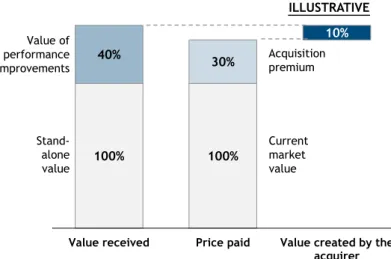
1.4.5. How to avoid the synergy trap
One of the main reasons for managers and investors to fall in the synergy trap is by not being able to oversee the above-the-premium price they pay for a deal. As illustrated by Koller et al. (2010), the value created by the acquirer is illustrated in the figure below, where if the acquirer is able to generate enough synergies above the premium paid to the business, he will be able to create value.
Figure 2 – Acquisition valuation framework
Koller et al. (2010) suggest that the value creation depends on two major factors: the performance improvements (or synergies) and the premium paid to the target company. As a result, we can compute the value created by the acquirer in the following way:
100% 100%
40%
30%
10%
Value received Price paid Value created by the acquirer Stand-alone value Value of performance improvements Acquisition premium ILLUSTRATIVE Current market value
(18) ( ) ( )
Hence, this formula will give us the foundations for the computation of the “meet the premium
line“(MTP) as suggested by Sirower and Sahni (2006). The MTP line is a helpful tool to understand if
investors are paying too much for the business and if they are being too optimistic.
Sirower and Sahni (2006) presents a formula that combines both efforts in costs and revenue synergies with the current profit margin and premium paid, thus, creating a frontier where the investor can “avoid the synergy trap”:
(19)
( )
In the example in figure 3, the authors have computed a scenario where a certain company is willing to pay a premium of 35% for a business with 18% profit margin. As a result, the amount of synergies generated to pay off the investment needs to be above the blue line.
Figure 3 – Meet the premium line
Let’s look, for instance point 1. In this point, the synergies are 8% cost efficiency gains and nearly 7.5% for revenue increases, which, by modifying formula (17), we see that the amount of synergies are above the premium paid.
) ⇔ ( )
⇔
On the other hand, case 2 and 3 don’t generate enough synergies for the premium paid, therefore, investors should “avoid the synergy trap”.
Furthermore, Sirower and Sahni (2006) suggest that firms are much better reducing costs than increasing revenues due to competitor’s response or customer’s reaction to the merger. As a result, following previous studies and benchmarks made by the authors, a 10% decrease in costs and 10% increase in revenues comes as a reference in calculating both types of synergies. As explained by Sirower and Sahni (2006) , when setting the parameters by the acquirer, the plausibility box helps investors to better triangulate and understand if they are being too optimistic on cost reductions or in revenues enhancements. 0% 3% 5% 8% 10% 0% 10% 20% 30% 40% 50% 2 1 3 %Syne rCo sts %Revenhanc ILLUSTRATIVE Plausible zone
The case of Vivo and TIM 19
2. Industry review and market assessment
The telecommunications industry is a broad market that throughout the past century has suffered numerous shifts. From the invention of the fixed voice line, the first steps in the world wide web, the mobile phone and lastly, the high speed broadband, it has enabled people to communicate more, better and change information faster. This industry was one sector where the companies had to adjust their business plans, invest huge amounts of money and keep innovating.
This chapter will be divided into five main categories: an introduction to the main telecom macro trends, data trends, the Brazilian market and the macro trends, how the telecom sector in Brazil is evolving and what we expect the Brazilian market to be in the next couple of years and, finally, a deep dive into Vivo and Tim service providers. We will conclude with a brief description of the revenue and cost drivers.
2.1. Global telecom trends
In this first chapter, we will take a look to the telecom landscape. How countries are evolving in the telecom space, take a brief look at the different rhythms per region, how the 2010’s decade is reshaping the telecom industry and what should be the next challenges and improvements for operators that want to boost their competitiveness.
Using data from wireless intelligence from February 2014, we have computed the correlation between GDP per capita at purchasing power parity and country penetration. As we can see in figure 4, purchasing power is a strong indicator of mobile penetration with an explanation power of 53%.
This correlation suggests that the higher the economic growth and development, the higher the propensity for mobile phone acquisition. The African continent is still the region with the lower mobile penetration, followed by the Americas (with the exception of US and Canada) and then the Asia and Pacific. On the other hand, Europe shows already a high penetration of mobile phones with almost all countries with penetrations above 100%.
Figure 4 – Correlation between GDP per Capita and penetration
Finland USA Brazil Mexico Argentina Portugal R² = 53% 10,000 20,000 30,000 40,000 50,000 60,000 0% 50% 100% 150% 200% 250% Africa Americas Asia Pacific Europe Middle East GD P p er ca p it a (U SD PP P ) Country penetration (%) Source: Wireless inteligence