Recommendation systems and other analytic methods

(1)

2019

UNIVERSIDADE DE LISBOA

FACULDADE DE CIÊNCIAS

DEPARTAMENTO DE ESTATÍSTICA E INVESTIGAÇÃO OPERACIONAL

Recommendation Systems and Other Analytic Methods

Ana Patrícia Martins Gonçalves

Mestrado em Matemática Aplicada à Economia e Gestão

Trabalho de Projeto orientado por:

Maria Teresa Alpuim

(2)

i

Acknowledgement

I would firstly like to thank my internship tutor, Ricardo Galante, for all the support, knowledge and trust that I have received in the begging of my professional path. Truly inspired me to always learn more and stay curious.

To my professor, Maria Teresa Alpuim, responsible for this project, thank you for all the motivation and support for coming in this new challenge.

To my family, thank you for the endless support along my 23 years. For always encouraging me to pursue what I like and for giving me the foundations of a good education.

To my friends, my second family, who accompanied me along this project and to whom I was able to share my experiences and laugh in good and bad times, I wouldn’t be the same person without being surrounded by you, with special attention to Mariana and Pedro.

To all my colleagues in SAS, I thank you for being so welcoming and making me feel part of the SAS family. With a special thanks to Bruna for sharing a first work experience with me in a new environment.

To the company where I did this project, thank you for all the opportunities given to me along this process, in particularly, the Pre-Sales Global Academy I attended in North Carolina, USA for roughly six months. It was a truly rewarding experience, on personal and professional levels. I was able to participate in a Data for Good project regarding the water access optimization in Central African Republic, which was a real example of how analytics can be used to help people.

(3)

ii

Abstract

In this report we will explain the fundamentals of Recommendation Systems and other analytical methods giving a more insightful vision on the analytical part. The goal is to give the reader an overall context on the topic, so it becomes comfortable to talk about it and the surrounding context. To start, we are giving an overview on the Analytics Life Cycle, because we need to understand what the steps are, to be able to move forward. After, there is also an insightful chapter about one of the hot topics nowadays is Machine Learning, therefore we will detail it a way that you can be familiarized with the basic approaches it takes. More to the core of the project, we talk about Recommendation Systems and which are the approaches taken to achieve them, which are the methods. Since models need data to be significant, we give a view on how we gather information for most recommendation systems, since it is a more specific case. Once we have the model, how do we know if it is good or not? There is always an evaluation metric, a way of knowing if an analytic model is performing well and accurately enough. Later, we talk about statistical bias. This is particularly important in the sense that, even though have a lot of data, if it is not independent, it will not provide clear and truthful insights. Giving that this is a report based on machine learning algorithms, other models are addressed as well: Decision Trees and Clustering.

Here at SAS, we say that when curiosity meets capability, progress is inevitable. Working with data can be difficult, from data cleansing to data model deployment, goes a long way. It is our mission to provide tools for data manipulation, that are easy for all to handle.

(4)

iii

Resumo

Neste relatório de projeto vamos explicar os fundamentos de Sistemas de Recomendações e outros métodos analíticos dando uma visão mais direcionada para a parte analítica. O objetivo é dar ao leitor um contexto geral sobre o tópico, de forma a que esteja à vontade com a linguagem associada. Para começar, vamos dar uma visão geral sobre o Ciclo Analítico, pois é necessário entender quais são os passos a dar para podermos avançar neste. Seguidamente, é também escrito um capítulo sobre um dos tópicos do momento, Machine Learning, portanto será descrito com algum cuidado para o leitor ficar familiarizado com as metodologias principais ligadas a esta abordagem. Mais direcionado para o ponto principal do projeto, falaremos sobre Sistemas de Recomendação e quais as abordagens utilizadas para o sucesso destes, quais os métodos. Visto que os modelos necessitam de dados para serem significantes, abordamos também como vamos realmente reunir os dados necessários para utilizar nestes. Uma vez tendo o modelo, é necessário avaliar se este é bom ou não. Existe sempre uma métrica para tal avaliação, uma forma de compreender se o modelo está a prever bem ou com a precisão suficiente. Mais tarde, falamos sobre enviesamento estatístico. Este tópico é bastante importante na medida em que é algo muitas vezes não é discutido e que por essa mesma razão, por vezes, pode levar a resultados errados, que não correspondem à realidade. Sendo este projeto baseado em algoritmos de

Machine Learning, outros modelos importantes são também explicados: Árvores de Decisão e Clustering.

No SAS, é usual dizermos que quando a curiosidade se junta à capacidade, o progresso é inevitável. Trabalhar com dados pode ser difícil, desde a limpeza destes até ao deployment, vai um longo caminho. É a nossa missão fornecer ferramentas para manipulação de dados, de forma acessível a todos.

(5)

iv

List of Figures

Figure 1 Data vs Oil ... 8

Figure 2 Analytics Life Cycle ... 9

Figure 3 Measures of Association Rules ..……….…..17

Figure 4 Market Basket Analysis Network Diagram ... 20

Figure 5 Market Basket Analysis Zoom-In Diagram ... 21

Figure 6 Full Decision Tree with SAS VA ... 25

Figure 7 Node in a Decision Tree in SAS VA ... .26

Figure 8 Path in a Decision Tree in SAS VA ... 26

Figure 9 Clustering subdivisions ... 27

Figure 10 Agglomerative Hierarchical Clustering ... 27

Figure 11 Divisive Hierarchical Clustering ... 28

Figure 12 K-Means Clustering vs Fuzzy C-Means Clustering ... 28

Figure 13 Example Dataset Plot ... 29

Figure 14 Example Clustering ... 29

Figure 15 Centroid in Clustering ... 29

Figure 16 Optimized Centroids ... 30

Figure 17 Euclidean Distance ... 30

Figure 18 Manhattan Distance ... 31

Figure 19 Cluster Polylines ……… 32

(8)

vii

List of Tables

Table 1 Incomplete Client Database Example by DataRobot ... 12

Table 2 Complete Client Database Example by DataRobot... 13

Table 3 Market Basket Analysis Dataset... 19

Table 4 Market Basket Analysis Results ... 20

Table 5 Sparse Data in Ratings ... 22

Table 6 User Ratings Patterns Example ... 22

Table 7 Movie ratings about features example ... 23

Table 8 Feature preferences example ... 23

Table 9 Calculated Ratings Matrix Example ... 23

Table 10 Random Features and Items Ratings ... 24

Table 11 Results of Ratings from Random Values ... 24

Table 12 Retail Dataset ... 31

Table 13 Cluster Summary ... 32

Table 14 Centroids Summary ... 33

Table 15 Iterations History ... 33

(9)

8

1. Introduction

Oil is no longer the most lucrative commodity in the world. This idea is becoming more and more popular as the years go by. Some years ago, questions related to oil regulations were the ones being addressed. If we look at today’s scenario, new questions about data regulations are appearing every day. This is mainly because when there is a very popular source of income, big companies take the opportunity and explore the most they can. Data is the new oil, but oil needs to be refined, and so does data.

Figure 1 Data vs Oil

In this report we show how data can be refined and used for better automatization. All this refinement will be done with the help of SAS Software, to assure better performance in time and quality. The order of the topics was chosen to give the reader a guided path end to end.

This project intends to give a clear idea on how recommendation systems work. To achieve that, there is some adjacent topics that should also be known. The project had a strong business-oriented approach, in the sense of making theorical things practical. Alongside with learning about the analytical methods, several customer meetings were also attended. It was a way to get an insight on how theory meets reality. We had some advances about recommendation systems, so that after a few months past the internship, it was customer ready. The other methods mentioned, such as Clustering and Decision Trees were also a very important part of how we can explain the patterns of data, in an intuitive way, to provide value to the customer. One great lesson taken from this is that there are no perfect models, but we need to make them as better as possible and this is acceptable since not everything lies by the same patterns. If we can take value from using Analytics, we are on a good track. It is a matter of improving and gathering more data (more materials) to work with it. Working with data needs resilience, and that is what a Data Scientist should have. Here at SAS, we try to make things more efficient and optimized, for the working team.

(10)

9

2. SAS Analytics Life Cycle

“But what is data? At its most general form, data is simply information that has been stored for later use.” (Nelson, 2019)

SAS covers the full analytics life cycle: Data, Discovery and Deployment. To work with data and make use of it, it is necessary to be able to do something end to end and for that, it’s always fruitful to combine all the tools in one interface, to facilitate and save time. Starting with the first step, Data, which is the foundation of the cycle, where it all starts. We need to retrieve data from different data sources, and this can sometimes cause problems because of different formats coming together. SAS Software can get data from multiple data sources such as Hadoop, Oracle Databases or Excel Worksheets. Once all the data are retrieved and transformed in SAS data sets, it is time to move to the second step,

Discovery. This phase is where our creative and exploratory sense takes part. Once the data is explored and analyzed, it is time to determine what changes or adjustments need to be done, such as, for example, handling missing values. The more statistical part follows, creating models that aim to produce data driven decisions about future actions. Let us say that we want to predict the probability of a customer churn, based on previous data bout this type of event. It is possible to train a model so that it can identify new clients for whom the same event is going to take place, in this case, to identify if the customer is going to churn. Once the model is defined, it must be put in production to be useful, and this corresponds to the last step of the process, Deployment. This is the phase where most open source software fails,

since it is not efficient neither in time nor scalability.

Figure 2 Analytics Life Cycle

“We are already overwhelmed with data; what we need is information, knowledge, and wisdom.” Dr.

John Halamka, CIO Beth Israel Deaconess Medical Center

How can we then handle the data to obtain insights? It is a process, so we have several phases to reach our goal. Below, we will look at the three foundations of Analytics.

(11)

10

2.1. Descriptive Analytics

“What has happened?”

In this first phase, we summarize raw data and make it interpretable for people. It is the most basic process of pattern discovery where we start looking for possible causes for the output data. Most of basic statistics are within this category, as for example, sums and averages. “Use Descriptive Analytics when you need to understand at an aggregate level what is going on in your company, and when you want to summarize and describe different aspects of your business.” (Descriptive, Predictive, and Prescriptive Analytics Explained, 2019)

It is so common to do this every day in most organizations that we do not usually put a label on it. A simple real-life example is their use in retail. Every day, there is a need to do reports on inventory, sales, costs among others. This is fundamental to assess the success of the business. If we can have a clear view on what is happening, we can adjust points to get better, at a very high-level approach. And this does not need any special algorithms, it is simply a visual display of what has happened. Take the example of a descriptive tool that we use through most of our lifetime. Bar charts are a simple but powerful visual tool. A frequencies analysis, which is the foundation of a bar chart, is usually learned in elementary school, however, it is one of the data scientist procedures used in fairly every area.

2.2. Predictive Analytics

“What could happen?”

For this second phase, we use statistics to try to understand future outcomes. As it is known, there are no perfect predictive models but still, if they are significantly good, it serves as an advantage.

Predictive Analysis is based on probabilities, while Descriptive Analysis is based on real historic data. When working with probabilities, an error is always associated, and the real effort is to try to minimize this error as much as possible and for that purpose there are various metrics that can help us understand the quality of the predictions. “Use Predictive Analytics any time you need to know something about the future or fill in the information that you do not have.” (Descriptive, Predictive, and Prescriptive

Analytics Explained, 2019). This will be the main point in recommendation systems, where we must predict ratings for user/item interactions that did not happen yet.

2.3. Prescriptive Analytics

“What should we do?”

For the third and final phase of what we are addressing, the analytics should provide advice on the best solution for the case under study. This is a very important step because Prescriptive Analytics attempts to quantify the outcome resulting from the use of a certain predictive model. We already have the model, now we want to know what is the best way to use it, how to put it “in production”? This is the final step on the analytics process: to be able to make decisions based on our findings.

(12)

11

3. What is Machine Learning?

This is a very common term in the current times since the technologic revolution is getting more and more considerable and companies need to adapt to the enormous volumes of data that are gathered every day. For that, we have the urge to turn unstructured data into value in terms of knowledge. How do we keep up with this evolution, this growing data gathering? It would cost more time and money if a company’s employees did all the analysis from scratch. Machine Learning is the solution, since it is a set of rules, procedures and fundaments, that allow machines (computers) to act and make decisions in a way that they are constantly learning from their “mistakes”, their errors. It differs from the explicit programming of a task, where the outcome is set, and the process procedures and parameters are static. So, in Machine Learning, the more data it comes along the way, the more accurate the model will be.

On another take, we can see machine learning as a system that can modify its behavior automatically according to the data that it is being fed with. This modification of the behavior is built on a set of logic rules that are ways of measuring how we can achieve the defined goal, that is, the target. Again, these rules are based on the acknowledgment of patterns in the data. As an example, imagine that someone writes a word, that has two means, in a search engine. Which one should be one prioritized? Based on the user historic, the system can determine what is more relevant, or what has been searched before, in a similarity sense.

Bottom line, what we want to do is extract information from our data to create smarter business decisions. The Analytics Life Cycle has the data ingestion and preparation, explorations and modeling for new predictive models. There is an urge to make this automated, because there are no feasible resources to do everything manually. Machine Learning is more necessary in the modeling part, but it is also present along all the process.

3.1. Unsupervised vs Supervised Machine Learning Algorithms

3.1.1. Supervised Learning

This is the most used type of machine learning algorithms. It relies on input variables (independent variables) and an output variable (dependent variable), which can be called as the “target”. The name of this algorithm derives from the process of which the machine learns to make predictions. We know beforehand the correct output (the dependent variable), therefore when the algorithm produces predictions on the training data, it knows whether the predictions are correct or wrong. So, it works as a teacher, in the sense that the model uses the independent variables, determinates their parameters, to achieve a value (dependent variable) and if the predicted result is not good (if it is significantly different from the observed value), then the model learns that the parameters should be reevaluated so that the predicted value is as close as possible to the observed value, i.e., to generate the smallest possible residual. This process stops when there is a good level of the model performance.

In a more practical way, an example of a supervised learning method is the logistic regression, which models the probability of a classification problem with only two outcomes, e.g. pass or fail (0 or 1) in an exam, taking into consideration the effect of other variables, which may be discrete or continuous. This method is a variation of the linear regression model, which relates a continuous variable with other variables, discrete or continuous.

(13)

12

3.1.2. Unsupervised Learning

The main difference from the above type of machine learning algorithm consists in the lack of a dependent variable (an output variable). The main purpose for the use of unsupervised learning is to discover hidden structure/distribution of data so that we can aggregate it in groups and further analyze it. We can also differentiate the types of problems considered in this method, i.e., Clustering and Association, being the first one used when there is a need to aggregate groups based on the data (very common in retail, to identify the different types of customers), and the second used to discover rules that relate data within the set (often used to find out what kind of products should be displayed closely in a shelf, since the customer that buys X tends to also buy Y). Clustering techniques will be mentioned along the report.

3.1.3. Semi-Supervised Learning

This type of learning is used when there is a considerable amount of input data and only some of it is labeled. It is a middle term between the two learning methods seen above, which is beneficial in the way that most real-world situations fall into the sparsity of information and there is a need to overcome those “data problems”.

A common example is when it comes to detect a fraud in banking transactions. Imagine we have a lot of accounts from customers and some we know that there is fraud, but others we don’t. Some of the data will remain unlabeled (with a missing value in the target variable), as you can see in Table 1 below.

Table 1 Incomplete Client Database Example by DataRobot

A way to handle this problem is to use a semi-supervised learning algorithm to fill the missing values and after, to train again the model with the “complete” dataset, as in Table 2.

(14)

13

Table 2 Complete Client Database Example by DataRobot

Now, we have a more complete dataset, however it is not totally accurate since we are working with predictions only. Semi- Supervised Learning methods are then an approach to complete a data set that does not have all observations with a label or target value.

4. Statistical bias

When collecting data, there is a special importance when it comes to selecting a random sample that can portrait the population in study, so that we avoid statistical bias that influence the future predictions and give a misconception of the model outcome. In this chapter we show, in a simple way to understand, some examples of statistical bias.

4.1. Survivorship Bias

It is a cognitive bias that happens when we try to infer a decision based only on past successes ignoring past failures. The predictions would then be too “generous”, not really portraying the reality.

A very important discovery related to this type of bias happened during the II World War. Abraham Wald, a mathematician saved many lives by creating an aircraft repair recommendation system. Instead of relying only on the data regarding the airplanes that came back damaged after being send out to the war, he took special attention to the ones that actually did not come back, and in fact, those last ones were the most important because it meant that they were more affected by the damages (to the point that they did not survive to come back to the base). So, to suggest where to repair or where to reinforce the aircraft, Wald noticed that the places where the aircraft that returned base were less damaged, were probably the ones that should be taken in more consideration for the future planes to send out. Thus, the airplanes that were hit in the parts that the ones that returned home were not, did not make it to count as case to take in account for the future recommendations. This problem is a very good example of how we should consider the data that we receive and the adjacent data that it is not directly explicit (referring to the case of the airplanes that didn’t come back and were not considered for the future events).

(15)

14 << U.S. Navy, in 1943: “We want to estimate the conditional probability that a plane will crash, given that it takes enemy fire in a particular location, in light of the damage data from all other planes. This will allow us to personalize survivorship recommendations for each model of plane. But much of the data is missing: the planes that crash never return.” >> (Polson & Scott, 2018)

4.2. Selection Bias

This is the most general form of bias. It indicates that we are working with a specific subset that does not represent the whole population. It can happen, when collecting only the data that is easy to access, leaving the “odd” cases uncounted. Take the example of sending a survey about a magazine, only to the readers of that magazine. Well, normally if the customers read/pay the magazine, it means they like it in the first place, otherwise that would not happen. This way, we are already narrowing our population and not portraying the most general case.

4.3. Recall Bias

This error is purely “human”. When asked for a survey, one might not remember his/her experience with the product or service with such precision. Take the example of the meal you ate 4 days ago. You probably have an idea on what it was and whether it was good or bad, but if you were asked to rate that meal on a 1 to 10 scale, how precise would you be? Recall bias is then, the error of not remembering with precision when answering a survey.

5. Recommendation Systems

What is the importance of providing support in decision making? More than ever, we live in a time where there are plenty of choices for everything you want to buy. Is that a good thing? It might be apparently beneficial for the costumer, but it is not for the seller. Let’s see an example from a study named When Choice is Demotivating: Can One Desire Too Much of a Good Thing? This was an experiment where there were two stands of jam on two different days. One stand had 24 different jams while the other had just six. The stand with the most variety only sold the jam to 3% of the customers who visited. The stand with the least variety sold the jam to 30% of the customers who visited. The difference of 3% to 30% is quite considerable when it comes to retail. Let us look at the reality in many sectors, such as the entertainment one. When someone turns on the television, the choices of a show to watch are “innumerous”. And since data, especially big amounts of data are now viewed as extremely

(16)

15 valuable, companies take (or plan to take) the most advantage of it to gain value. Now, let us see some numbers to really take consciousness of what is happening:

• At Netflix, 2/3 of the movies watched are recommended

• At Google, news recommendations improved click-through rate (CTR) by 38% • For Amazon, 35% of sales come from recommendations

When well implemented, recommendation systems are extremely valuable to a company. However, they cannot perform well if there is not enough data (this is the case for any model in machine learning, but some are more sensible to it). Why is that? People usually say that knowledge comes from

experience, and in fact, that is the case for model making. We should always remember that the more records/observations/information we have, the easier is to identify patterns, predict events, and ultimately to have a higher accuracy in the data-driven decisions we are taking. This is so because, for example, trends can be a one-time deal and if we infer something only based on, let’s say, last year trend, the predictions will be not, by any means, reliable. Before we jump on any model making, there should be an extra consideration on having enough data, in quantity and variety, to work with.

5.1. Data Used in Recommendation Systems

There are different types of data that are clearly useful when building a recommendation system and

we will describe four of them, being among the more frequently used.

5.1.1. Rating data

Rating data refers to the evaluations/ratings the user makes, and it can take different forms such as negative/positive comments (discrete variable) or high/low ratings (continuous variable).

5.1.2. Behavior Pattern Data

Behavior Pattern Data refers to what the user did unconsciously when shopping. This can take many forms such as, duration of browsing, click times, refresh of webs, selection, copy, paste, bookmark and even download of web content. It relates to the user’s interest and hesitations when looking for something, with the intent of shopping.

5.1.3. Transaction Data

Transaction Data is the most quantifiable and direct type of data that can be gathered. It can be the purchasing date, the purchased quantity, the price or even the discount on the item.

(17)

16

5.1.4. Production Data

Production Data refers to the details involved in an item. Let us say that for movies, the production data consists in the actors, the topic, the release time, the price of the set and the director, among others. It is the set of features inside the product.

5.2. Information Gathering

To build a model, we need to have data to work with. For this case, if we talk about recommendations, it is expected that our dataset will have at least three variables: the user identifier (client), the items (products) which the user ranked, and, of course, the ranking given by the user to the item. Other variables can also be taken into consideration, however, in a more straightforward approach, the essentials are really the ones written above. Since not every user bought every item, therefore, did not rank every item, we can have some missing values in those user-product rankings. To tackle that issue, when it comes to make mathematical operations, there is a method suitable to handle those missing values, Factorization Machine. We will address it later in this report.

5.2.1. Explicit Feedback

This is, as the name implies, the most straightforward way to collect ratings from the user’s profile. This is achieved usually through forms or platforms used for gathering data introduced by the user. Also, a point worth to refer is that the interests of a user can be achieved through their “favorites”, being an explicit form as well.

This type of information gathering can, sometimes, present some problems. Imagine the last time you bought something online. After the purchase, you were probably asked to rate the transaction and most probably, you did not have the time or the patience to do it. In fact, it can be very hard to persuade a customer to review an item after he bought it. Also, some people are very reticent to provide personal information for something that is not necessary, so more complex forms discourage their filling. Lastly, we have no guaranty that the information gathered is correct or corresponds to the truth, we just assume it.

5.2.2. Implicit Feedback

In this type of feedback, it is mandatory to observe the interactions the user had with the system. These interactions can be, for example, the time of visualization and the selected items. Based on historic records of the user’s interactions, we can find some behavior patterns that will be used to predict the customer interests. Contrary to the previous feedback type, here we do not need to ask anything to the customer, which is an advantage. On the other side, one limitation is that we can only get positive feedback, because every interaction is considered an interest of the customer. Therefore, it is not that clear to find what items are considered bad, instead of neutral.

(18)

17

5.2.3. Hybrid Feedback

Finally, this type of feedback combines both Explicit feedback and Implicit feedback, to get the strengths of each one and minimize their weaknesses. An example of this is allowing the user to provide explicit feedback only when he expresses interest (through implicit feedback).

5.3. Filtering Techniques

5.3.1. Association Rules

Association Rules recommend items based on their place along with different products. If we buy two products together, they are linked in the same transaction. The association rules between an item X and an item Y, can be measured based on support (s) [1], which consists on estimation of the probability of buying X and Y simultaneously, knowing that a buying was made and confidence (c) [2], which consists on the estimation of the probability of buying Y, given that X was bought. To translate this concept into an equation, we have:

𝑠 =𝑛𝑢𝑚𝑏𝑒𝑟 𝑜𝑓 𝑡𝑟𝑎𝑛𝑠𝑎𝑐𝑡𝑖𝑜𝑛𝑠 𝑐𝑜𝑛𝑡𝑎𝑖𝑛𝑖𝑛𝑔 𝑋 𝑎𝑛𝑑 𝑌 𝑡𝑜𝑡𝑎𝑙 𝑛𝑢𝑚𝑏𝑒𝑟 𝑜𝑓 𝑡𝑟𝑎𝑛𝑠𝑎𝑐𝑡𝑖𝑜𝑛𝑠 [1] 𝑐 =𝑛𝑢𝑚𝑏𝑒𝑟 𝑜𝑓 𝑡𝑟𝑎𝑛𝑠𝑎𝑐𝑡𝑖𝑜𝑛𝑠 𝑐𝑜𝑛𝑡𝑎𝑖𝑛𝑖𝑛𝑔 𝑋 𝑎𝑛𝑑 𝑌 𝑛𝑢𝑚𝑏𝑒𝑟 𝑜𝑓 𝑡𝑟𝑎𝑛𝑠𝑎𝑐𝑡𝑖𝑜𝑛𝑠 𝑐𝑜𝑛𝑡𝑎𝑖𝑛𝑖𝑛𝑔 𝑋 [2]

5.3.2. Content-Based Filtering

This technique is based on the analysis of the attributes of items to generate predictions. The recommendation here is made based on the user profiles with features from the content of the items that the user ranked before. So, content-based filtering is based on item similarity and not on user similarity.

5.3.3. Collaborative Filtering

This technique is used for content that cannot be described properly by metadata such as movies or tv shows. It consists on creating a user-item matrix, made of preferences for items by users. Then, matches users with relevant interests through calculations regarding similarities between the users’ profiles. Those users create a group called neighborhood. After that, a user receives recommendations

(19)

18 to the items that he has not yet ranked. Basically, this type of filtering uses user similarity instead of item similarity.

5.3.4. Hybrid Filtering

This technique consists in using different recommendation types of filtering, to get some improvements from using one technique only.

5.4. Evaluation of a Recommendation System

Once the variables and the model are chosen, we need to divide the users of our data set in two sets. The first one is the training set, which consists in the data used to first train the model, discover patterns and associations between the items. This training set usually consists of 80 percent of all the data we have. The other 20 percent is used to test how the model performs on new observations, unseen ratings, in our case. This last data set is called test set and it is used to simulate how it would work in a real context. We test now different users and see whether the suggestions/recommendation are accurate with the actual rating. Firstly, we hide the result, in this case, the ratings that we want to predict, and after we evaluate if the predictions match with the real ones that were hidden. Ideally, we want the predicted to be the same as the actual. The way that we compare those is with root mean squared error (RMSE), a measure of the differences between values, the predicted and the actual. A RMSE of zero would mean a perfect fit but, that is very uncommon. For that, we should give preference to a lower RMSE, as close to zero as possible. The lower it is, the more accurate.

5.5. Approaches to create the model

In this chapter, we will present two approaches used in recommendation systems, namely, Market Basket Analysis and Factorization Machine. Note that these are not the only possible ways, as there are many other complex methods to obtain the same goal. Why did we choose these two? They will be the focus since Market Basket Analysis is the most traditional approach and Factorization Machine is the most modern approach. We can then see how one has the fundaments and the other has also the solution for the gaps in the previous.

5.5.1. Market Basket Analysis

This is an analytical method often used to search similarities between the purchase of items. It consists in association rules, to better predict which products will likely be bought together. For retailers, this is the goal when it comes to cross-sell (selling an additional product to a usual customer). For example, if somebody buys cereals, then the likelihood of them also buying milk is high. This approach

(20)

19 is mostly based on frequencies, that is, the amount of times people buy the products together, as in the example presented in Figure 3.

Figure 3 Measures of Association Rules

The way to evaluate if a rule (e.g. buying product X, implies buying product Y) is relevant is based on three measurements: Support, Confidence and Lift. The first two were already explained in section 4.3.1. The only new concept here is Lift. This value is a way to measure the importance of a rule and it can only take positive values, with the value 1 corresponding to the case where X and Y are

statistically independent. Values less than 1 mean that X and Y have a negative correlation and bigger than 1, that they have a positive correlation.

Although most times we hear about this approach regarding retail sales, it can also be used for telecommunications and insurance, for example. For the first one, it is mostly used to reduce churn (customers in risk of not being a customer in the future) rates in the way that one can identify which products are being bought together and which profiles can we target to retain those customers by providing a better customer experience. In insurance, we can more easily detect fraud by analyzing the profile of claims being reported. It is easier to inspect whether a pattern of claims is uncommon, to further compare with other similar cases.

5.5.2. Market Basket Analysis Use Case

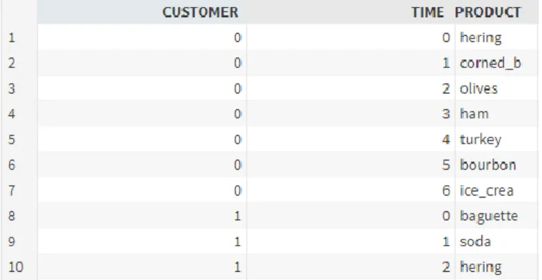
For this use case, we will look at data from a supermarket (purchases), for a certain number of months. Since we are dealing with data illustrating individual purchases, there is a need for it to be transactional, with one row for each observation, for each purchase. In the following sample of a dataset, we have three columns (variables): Customer, which represents the transaction ID; Time, corresponding to the time of the purchase and Product, being the description of the item purchased. A part of the dataset mentioned can be seen in Table 3.

(21)

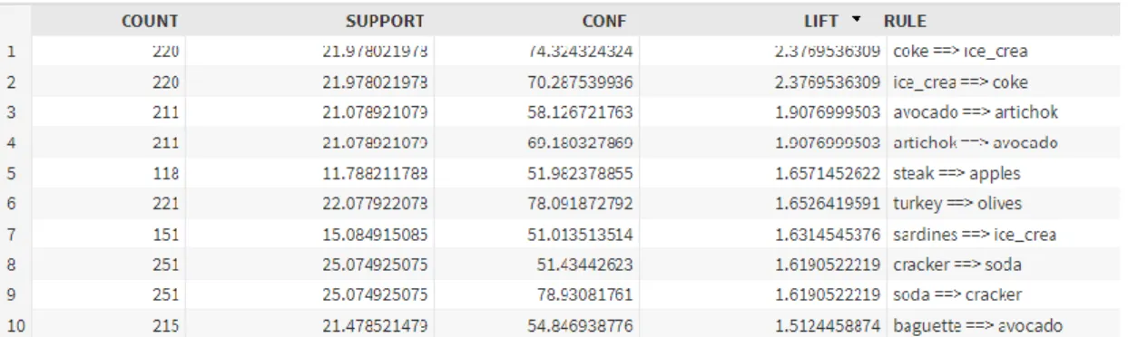
20 The actual algorithm is then called using a SAS procedure (a group of SAS statements that call and execute a procedure, a PROC step) named MBANALYSIS, which has intellectual property owned by SAS. This procedure is going to produce several Association Rules using the lift metric, to assess whether a rule is significant or not. Table 4 shows an output of the top ten association rules (measured by the lift).

From the analysis of table 4, we can see that, for example, avocado and artichoke appear together 211 times, with a lift of approximately 1.9. This last number means that if a customer buys avocado, he is 1.9 times more likely (than customers who do not buy avocado) to also buy artichoke. In that case, the rules associated with those items go both ways (the ones who buy avocado are more likely to also buy artichoke as the ones who buy artichoke are also more likely to buy avocado) but that is not always what happens. To illustrate that, we can also see that customers who buy steaks are 1.65 times more likely to also buy apples. However, this probability is not the same for the opposite case. Steaks imply apples but apples do not imply steaks, in the same way.

The challenge now relies on evaluating all these rules from a large database. The best way to visualize it is by doing a network diagram using SAS Visual Analytics, shown by figure 4.

Figure 4 Market Basket Analysis Network Diagram Table 4 Market Basket Analysis Results

(22)

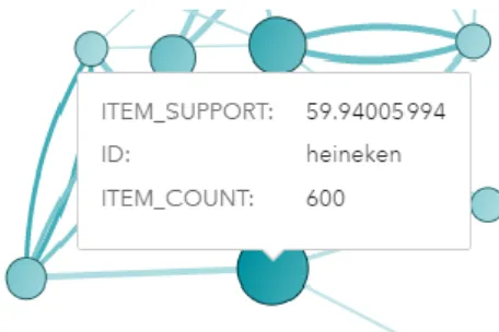
21 The size of the circles indicates the item count (the number of purchased items of that kind), the bigger the circle, the bigger amount of those items purchased. The circles color represents the item support (see chapter 4.3.1.), the darker it is, the higher support it has. Now, for the arrows connecting the items, the color represents the lift (the darker it is, the higher the lift) and the width represents how many times those purchases were made. Figure 5 shows an example where we can see that the heineken item was bought 600 times and that it was purchased in 59.9 percent of all those times.

Figure 5 Market Basket Analysis Zoom-In Diagram

Factorization machine (explained in the next topic) is more focused on the user/client and Market Basket Analysis is more focus on the item. So, we can combine both by seeing which product is more appropriate to a specific user and then, by seeing the items similarity (in terms of patterns of the buying), try to upsell some other products.

5.5.3. Factorization Machine

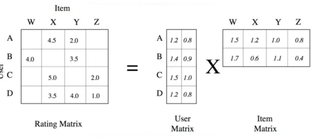
Factorization Machine is a supervised machine learning technique. The major advantage of this method relies on the power of reducing dimensionality problems by doing matrix factorization. In fact, it can be used on both classification or regression problems (categorical or continuous variables, respectively). In our main subject, recommendation systems, the amount of data necessary to perform well is tremendous. However, even though the combination of user and items is very large, not all users classify every item, so there are a lot of missing values in the process. The matrices table 5 illustrate the situation addressed before.

(23)

22

Table 5 Sparse Data in Ratings

Here, what we want to predict are the missing ratings. The affinity between users and items is modeled as the inner product between two vectors of features, one for the user and another for the item. These features are known as factors. We should associate the latent features that determine how a user rates a movie. In SAS, we can simply choose this method in a drag and drop interface (see Appendix), so that the modeling part is not an issue.

What challenges come with this? In real life, data are not static in the sense that people’s needs, and preferences are in constant change. To take those factors in account, it is important to use algorithms incorporating a time decay function and acknowledge the existing offer bias.

To make it clearer, let us look at the following new matrix in table 6, with information about how each user (Kelli, John and Martha) rated each movie (M1, M2, M3 and M4). This kind of matrix with no missing values is what we want in the end. But for this explanation, the following will help understands how the columns and lines work together. For example, Kelli rated M1 with 2 points.

Table 6 User Ratings Patterns Example

According to the table 6, we can see that there are a few dependencies among columns and/or rows, such as, Kelli and Martha have given the same ratings to the same movies. This does not mean that they are the same person, but it means that their taste is very similar. Another example is M2 and M4, once these two columns have the same values and yet, it does not mean that those two movies are the same, but they might be very similar, and people gave them very similar ratings. Now, how do we discover more underlying dependencies in the matrix? The answer is factorization matrix.

First, what is factorization? Imagine you have the number twenty-four and you also know that six times four is twenty-four. Six and four are small numbers but the product of them is a “big” number. This is the foundation of the factorization concept, where we have a large complicated matrix of ratings, in our case, and we want to decompose it into two smaller matrices.

So, the ratings matrix is given, and our task is to create two smaller ones whose product is the original one. This can be achieved by using features, so for example, when it comes to movies, one can have features like the following ones: Is it comedy? Is it action? Does it have luxury cars? Does it have boats? Is Ryan Gosling in there? It can almost be anything. To simplify, we will take the example of

M1 M2 M3 M4

Kelli 2 5 5 5

John 4 3 1 3

(24)

23 only two features: comedy and romance. The dot product is a way to guess a rating based on how much a user likes comedy and romance and how much a movie contains comedy and romance.

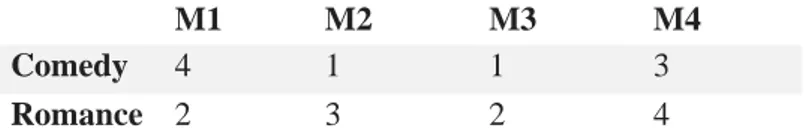
Now, let us also look at a matrix (table 7) containing the ratings for each movie, according to the features: comedy and romance. And another (table 8) containing users’ preferences to the features we are studying.

Table 7 Movie ratings about features example

Table 8 Feature preferences example

Taking Maria as an example, we know by table 8, that she likes comedy movies but does not like romance ones. Since movie M2 has a rating of one for comedy and a rating of three for action, we can start our inference. What we do here is adding the ratings correspondent to the features that the user likes. In this case, since Kelli does not like romance, the predicted rating is 1 because we are only taking in account the movie rating on comedy. If she liked romance as well, the rating would be 1 plus 3, which would be four. Basically, we are going to add the corresponding ratings that appear as a “yes” from the users’ preferences. Taking “Yes” as 1 and “No” as 0 in Features Preferences Matrix, we can now get the product matrix of the table 8 (considering it with ones and zeros, as mentioned above) with the table 7, which is the table 9 below.

Table 9 Calculated Ratings Matrix Example

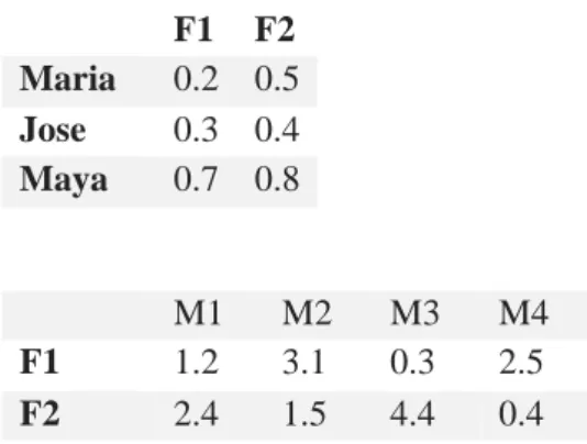
How do we get to find those two matrices of user features and items features? As in many problems, we start with random values until we get better and better results that will provide an appropriate value of reality. To exemplify, we could start with the random values for feature 1 (F1) and feature 2 (F2) as in tables 10. Remember that features can be, for example, the type of movie, comedy or romance. M1 M2 M3 M4 Comedy 4 1 1 3 Romance 2 3 2 4 Comedy Romance Maria Yes No Jose No Yes

Maya Yes Yes

M1 M2 M3 M4

Maria 4 1 1 3

Jose 2 3 2 4

(25)

24

Table 10 Random Features and Items Ratings

The result of multiplying the two matrices in table 10 is the matrix in table 11 below.

Table 11 Results of Ratings from Random Values

Now that we have our values, how can we evaluate if those predictions are accurate? That is where the error function gets into the picture. The computer program uses the error function to measure the accuracy of the predictions produced by this matrix product. Using the movies example, we will compare now the produced matrix with the original one, in other words, compare the values of table 11 with the values of table 9.

As we can see, the predicted rating of Maria about M1 is 1.44 (table 11), however the actual rating given is 4 (table 9). To measure this among all the other ratings we can do a simple calculation of the prediction error, namely,

Error = (actual – predicted)2

and this way, identify the more inaccurate predictions. This information will be fed into the algorithm and the way to decrease this error is by using another method called Gradient Descent which will work with the derivates of the error. However, this method goes beyond the scope of this project and will not be discussed here.

SAS also has a procedure that does Factorization Machine. However, the algorithm is intellectual property, so it cannot be shared here. Bottom line, our goal with this method is to get the full matrix with predictions for the missing values. The way to know whether our predictions of the missing values are accurate is by testing if the predictions on the values which exist, correspond to the real ones. If those do, then our features matrices have good values for the later multiplication of them, to get the desired ratings/user values.

F1 F2 Maria 0.2 0.5 Jose 0.3 0.4 Maya 0.7 0.8 M1 M2 M3 M4 F1 1.2 3.1 0.3 2.5 F2 2.4 1.5 4.4 0.4 M1 M2 M3 M4 Maria 1.44 1.37 2.26 0.7 Jose 1.32 1.53 1.85 0.91 Maya 2.76 3.37 3.73 2.07

(26)

25

6. Other Analytic Models Using SAS

6.1. Decision Tree

We will see a brief overview of this very popular method. Let us start with a general perspective:

have you ever seen a flow chart? A flow chart is a set of options that are made based on the previous option taken. If there is no loop, we can imagine a flow chart being a decision tree. In a decision tree you have branches and nodes which represent different things. The branches are the connections between the nodes and all the connections are derived from the root node (the first one with the overall information, not split in segments). In a decision tree, the path from the root node to the final node to be analyzed is the decision. This ultimate decision involves all the middle tier decisions that led to that. To make this clearer, let us think about a use case regarding a bank deciding whether they should give or not a loan to a specific customer.

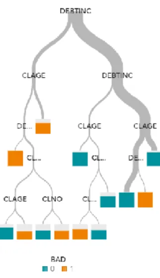
For the decision tree below, the independent variables to consider are DEBTINC (Debt to Income ratio), CLAGE (Credit Line Age), CLNO (Credit Line Number) and the dependent variable is BAD (determining whether the loan will be payed (1) or not (0). Note that for this example, knowing in detail each of the variables is not crucial for the explanation. The decision tree is formed by nodes chosen according to their importance to the model outcome. Our example, figure 6, illustrates a simple decision tree. With this, the first splits will be the ones with the most important variables, i.e., the ones influencing more the dependent variable. In the figure 7 we can see that DEBTINC is the most relevant variable for this case, being the first split in the process. Different branches come up and if we want to select a specific path, it allows to discover all the splits made to get to that point, figure 8.

(27)

26

Figure 7 Node in a Decision Tree in SAS VA

Figure 8 Path in a Decision Tree in SAS VA

Why is this method so popular among data scientists? Interpretability is key and this privileges that important quality. Decision trees present a clear path of the possibilities one can take, when going level by level to decide. They often mimic the human level thinking, so it is simple to understand the data and make realistic interpretations. They are not one of the called “black box methods”, where you can only see the result, not the process and steps that took you to get there.

How can we compare Decision Trees and Regression? These two methods have some similarities where target values are associated with multiple input values to create an association and predict new target values based on new input values. Both these methods aim to show a relationship between inputs and a target, they are not processed the same way. “Regression works by manipulating an entire matrix of information that contains all the values of all the inputs against the target and that attempts to compute an optimal form of the relationship that holds across the entire data set. Decision trees proceed incrementally through the data. Because of this approach, a decision tree might find a local effect that is very interesting and would be missed by regression.” (deVille, Barry; Neville, Padraic).

(28)

27

6.2. Clustering

This is one of the unsupervised machine learning algorithms. The goal of this method is to group similar points (data) in a way that we can discover underlying patterns and infer at groups of similar features. We can divide clustering in hierarchical and partitional. A brief overview of these methods will be given, with more emphasis on the most used algorithm. Within Hierarchical and Partitional, we can even subgroup again in other 2 groups, as seen in the figure 9 below.

Starting with the Hierarchical Clustering, this method uses a tree like approach. Within this class of algorithms, Agglomerative Clustering takes a “bottom up” approach, since it starts with each observation being a cluster and then, step by step, it merges those clusters into increasing larger ones. An example can be seen in figure 10, considering that each circle represents a cluster and the numbers represent observations.

Clustering

Hierarchical

Agglomerative Divisive

Partitional

K-Means Fuzzy C-Means

6 7 8 9 5 4 3 2 1 1 2 3 4 5 7 8 9 1 2 3 4 5 1 2 3 4 5 6 7 8 9

Figure 10 Agglomerative Hierarchical Clustering Figure 9 Clustering subdivisions

(29)

28 On the other way around we have Divisive Clustering, which uses a “top down” approach. It starts with a super cluster containing all observations and then the method splits the previous clusters in successively smaller clusters. A similar example to the one presented in the other type of Hierarchical Clustering is presented in figure 11.

Moving now to the Partitional Clustering, as it is the case of K-Means Clustering where the observations are divided into a previously defined number of clusters, the “k”. In this process, each observation belongs to exactly one cluster, not several. As this is, probably, the most common way of performing Clustering, we will explain it further along

The other Partitional Clustering technique mentioned is Fuzzy C-Means. This is very similar to K-Means in the way that it joins observations that have similarities among each other. The difference is that in this method, one observation can belong to two clusters or more, instead of just one, as in the case of K-Means.

Now that we have a view on what those methods consist of, let us look in more detail to K-Means Partitional Clustering. Take the example where we have a dataset with x and y coordinates, x corresponding to leg length and y corresponding to arm length. We are analyzing athletes and our goal

1 2 3 4 5 6 7 8 9 1 2 3 4 5 6 1 2 3 4 5 7 8 9 1 2 3 4 5 7 8 9

Figure 11 Divisive Hierarchical Clustering

(30)

29 is to cluster this data using k-means. Figure 13 shows a plot using a few observations just to exemplify the goal.

We will separate these datapoints into two clusters (figure 14). For the first one chosen (orange circle), we can see that it has players with a long arm and short legs. For the second one (blue circle), it is visible that the players there have a short arm and long legs.

So, how does this work? Firstly, two centroids are assigned randomly (represented by a triangle and a diamond in the illustration in figure 15, on the left). Then, the Euclidean distance (for example) is used to find which centroid is closest to each data point. Those points are then assigned to the correspondent centroid (illustration below, on the right).

Figure 13 Example Dataset Plot

Figure 14 Example Clustering

(31)

30 The next step is to actual optimize the initial clusters, so that those centroids are the in the central position of each cluster. This process is repeated so that the distance of the data points in the clusters to the centroid is as low as possible, as seen in Figure 16.

Going back to the problem of how to measure the distance between points, how can we do it? We need to evaluate the similarity between each pair of points or dissimilarity (how different they are from each other). This creates a distance matrix where we can assess what is the best pairing we can do to minimize distances. The most common methods of calculating distances in clustering are Euclidian distance and Manhattan distance.

The Euclidian distance is the simple straight line between two points, in the Euclidian space. The formula to calculate it is presented below, and figure 17 represents this distance in a system of axis,

𝑑𝑒𝑢𝑐(𝑎, 𝑏) = √∑(𝑎𝑖 𝑛

𝑖=1

− 𝑏𝑖)2 where a=(a1,a2,...,an) and b=(b1,b2,...,bn).

The Manhattan distance is the sum of the absolute value of the differences of the horizontal and vertical components. Like the Euclidian distance, the formula and the graphical representation for observations with n components are given below and in figure 18.

(a1, a2)

(b1,b2)

Figure 16 Optimized Centroids

(32)

31 𝑑𝑚𝑎𝑛(𝑎, 𝑏) = ∑|(𝑎𝑖 − 𝑏𝑖)|

𝑛

𝑖=1 where a=(a1,a2,...,an) and b=(b1,b2,...,bn).

6.2.1. Use Case

A very common use case in retail is targeting customers for better marketing campaigns. For this case we have a data set containing some information about customers of a specific retail company. The variables involved here, for every customer in the data set, are: Gender, Geographic Region of their address, Loyalty Status of their loyalty card, Affluence Grade (the average number of times they visited the shop in their region, per month), Age, Total Spend (the average amount of money spent in the shop of their region, per month). For this case, we used 15000 observations. The table 12, below, shows a sample of those observations.

Table 12 Retail Dataset

(b1,b2)

(a1, a2)

(33)

32 Now, what we want to do is group those customers in clusters so that we can target them as groups, in a more efficient way than just a general campaign, for example. To do that, we can use SAS Visual Statistics to, in a very user-friendly approach, drag and drop, see what the optimal clusters are. By default, the number of clusters given is five. Below, we can see in figure 19 a representation of the distribution of the customers within the clusters. Each color represents a different cluster and the lines along represent the path the cluster takes. For example, cluster number 5, in yellow, gives us the following information for its group of customers: both genders are in it but predominantly more females than males (we know the frequency of each category by looking at the thickness of the lines), the geographic region associated is mainly South East, the more common loyalty status is Gold, the affluence grade is medium and the age goes for older customers.

Figure 19 Cluster Polylines

Once we understand the paths, we can look on the cluster’s information/summary, as it follows in table13. For cluster 5, we have used 3472 observations/customers, the minimum Euclidean distance from an observation to the centroid is around 0.0192, the maximum Euclidian distance from an observation to the centroid is around 10.167, the cluster more similar to this one is cluster 3, the centroid Euclidian distance from cluster 3 to cluster 5 is around 2.75, the average Euclidian distance between observations and the centroid is around 1,67.

Table 13 Cluster Summary

Doing a further analysis on each centroid of the clusters, we can see are the predominant features, or if we are talking about continuous variables, what is the average of those. For example, in the table 14. Below, we can see that the centroid in cluster 5 is mainly about females, in the Midlands, with the loyalty status Gold, an average of 10.46 times Affluence Grade, average of 64 years old and average of 5829.8 Total Spend per month.

(34)

33

Table 14 Centroids Summary

The process of choosing the centroid was made iteratively. Since we want the want the minimum distance possible between observations and their correspondent centroid, below in table 15, we have a sample of the iterations made before achieving the best location for the clusters and centroids.

Table 15 Iterations History

Ultimately, we are now going to know which cluster is directed to each cluster. That is our main goal, knowing that we can target now similar customers (each cluster) according to their different features. For example, the table 16 below is a sample of where each customer is now allocated, when it comes to the determined clusters.

(35)

34

7. Conclusions

This project was a very rewarding experience, aside from the technical part learned, and the business knowledge acquired was, in my perspective, the most valuable. It is very important to understand the value of data in all phases, from data gathering to prescriptive actions or strategies based on advanced analytics techniques. In the case of market basket analysis, studied with more detail in this project, knowing which items are bought together, or the likelihood for that to happen is crucial to have a better shelf management, increase cross-sell and by doing that, increase revenue. On another take, if we have a challenge with sparse data, using factorization machines can be the solution. This, since when working with recommendation systems we face a lot of missing values and there is a need to fill those gaps with predictions of recommendations for the specific user/item pair in order to make recommendations regarding those combinations. Besides these two methodologies more oriented to recommendation systems (market basket analysis in a less focused approach and factorization machines in a more personalized and specific approach to a broader range), in this project I also learned about decision trees and clustering techniques. Regarding the first, the major advantage is to be a white box method, meaning that it is very intuitive and transparent along the process. The use of this method allows to understand the path to the accuracy of predictions we want to achieve, and which variables and values are relevant for outcome predicted. Last but not less important, the final topic was clustering. This methodology is probably one of the most usual ones among retail, commonly used for marketing campaigns. It was very insightful to see how a wide variety of customers has similar patterns that can be used to create targeted advertisements. In a time where information and data are abundant, it is crucial to have tools to handle it. Also, I could understand the technical knowledge alone is not very useful as it must be combined with the so-called soft skills. To create a balance between the two types of knowledge is the key for nowadays business environment. I learned a lot from both sides, and I value them equally.

(36)

35

8. Bibliography

(19, July 19). Retrieved from SAS: https://blogs.sas.com/content/hiddeninsights/2017/09/18/platform-architecture-for-ai-analytics-lifecycle/

(19, July 19). Retrieved from The Economist: https://www.economist.com/leaders/2017/05/06/the-worlds-most-valuable-resource-is-no-longer-oil-but-data

(19, July 19). Retrieved from https://towardsdatascience.com/a-gentle-introduction-on-market-basket-analysis-association-rules-fa4b986a40ce

(2019, June 6). Retrieved from Level Cloud: https://www.levelcloud.net/why-levelcloud/cloud-education-center/advantages-and-disadvantages-of-cloud-computing/

(2019, July 29). Retrieved from SAS: https://www.sas.com/en_us/customers/sobeys.html

(2019, January 2). Retrieved from https://ac.els-cdn.com/S1110866515000341/1-s2.0-

S1110866515000341-main.pdf?_tid=14d43c94-897f-498b-9b7e-c035ca5ae3ab&acdnat=1542902017_c6422e6355d351abd6c6f99d6b9ae020

(2019, September 16). Retrieved from DataRobot: https://www.datarobot.com/wiki/semi-supervised-machine-learning/

Alecrim, E. (2019, July 3). Technoblog. Retrieved from https://tecnoblog.net/247820/machine-learning-ia-o-que-e/

Choudhary, A. (2019, February 3). Retrieved from Analytics Vidhya: https://www.analyticsvidhya.com/blog/2018/01/factorization-machines/

Descriptive, Predictive, and Prescriptive Analytics Explained. (2019, January 10). Retrieved from Halo:

https://halobi.com/blog/descriptive-predictive-and-prescriptive-analytics-explained/

Khan, S. (2019, September 23). Retrieved from Quora: https://www.quora.com/What-is-the-difference-between-k-means-and-hierarchical-clustering

Kramer, A. (2019, September 19). Retrieved from

https://blogs.sas.com/content/sgf/2018/01/17/visualizing-the-results-of-a-market-basket-analysis-in-sas-viya/

Nelson, G. S. (2019, June 1). Retrieved from SAS:

https://www.sas.com/storefront/aux/en/spanlctkt/70927_excerpt.pdf

Pendergrass, J. (2019, June 6). SAS. Retrieved from

https://support.sas.com/resources/papers/proceedings17/SAS0309-2017.pdf Polson, N., & Scott, J. (2018). AIQ. Bantam Press.

Reddy, C. (2019, September 16). Retrieved from Medium:

https://towardsdatascience.com/understanding-the-concept-of-hierarchical-clustering-technique-c6e8243758ec

Saggio, A. (2019, July 12). Into the world of clustering algorithms: k-means, k-modes and k-prototypes.

Retrieved from AMVA4NewPhysics:

https://amva4newphysics.wordpress.com/2016/10/26/into-the-world-of-clustering-algorithms-k-means-k-modes-and-k-prototypes/

Simon, J. (2019, September 1). Retrieved from Medium: https://medium.com/@julsimon/building-a-movie-recommender-with-factorization-machines-on-amazon-sagemaker-cedbfc8c93d8

(37)

36