Scaling returns: a constant volatility strategy
Ana Filipa Moiteiro Andrade Ferreira
152412029
Abstract
This dissertation shows that scaling asset value-weighted returns from the S&P 500 index increases the Sharpe ratio of the portfolio from 0.19 to 0.62. The average Sharpe ratio for twelve value-weighted industry portfolios similarly increases from 0.39 to 0.72. Maintaining a constant level of volatility over time proved to hedge the investors risk and we show that using this constant measure of volatility over time, which corresponds to the historical measure of average volatility for the S&P 500 index, yields results robust across different indexes, sub-samples, across industries and for different sample restrictions. Robustness was also tested for recession and expansion periods, with the results being stronger for the latter. Finally, we compute a winner minus loser momentum strategy where the Sharpe Ratio of the strategy increases from 0.28 with raw returns to 0.65 with scaled returns.
Supervisor: Professor José Faias
Dissertation submitted in partial fulfilment of the requirement for the degree of International MSc in Finance, at Católica Lisbon School of Business and Economics, August 2015
Acknowledgments
Writing this Dissertation was undoubtedly one of the biggest challenges I faced so far in my life. Being able to do so required a great amount of effort and dedication and to be able to achieve such result I cherish and am thankful for all the help and support I received from several people along the way.
First I would like to express my gratitude to my supervisor, Professor José Faias. Thank you, above all, for your patience, dedication, constant availability as well as great feedback you gave me and, most importantly, for always pushing me to achieve my full potential.
Additionally, I want to express my sincere thank you to my colleagues from the Transaction Advisory Services department at EY for all the support and understanding throughout the last months. Likewise, I acknowledge “Fundação para a Ciência e Tecnologia” for financial support under the project PTDC/EGE-GES/120282/2010.
I also thank Ana, Alex, Afonso Diégues and Afonso Gonçalves. For being an essential part of my path at Católica during the last two years, your never-ending support and meaningful friendship somehow, I am sure, made this dissertation easier to write.
Finally, I would like to mention my family. For always believing in me and for constantly inspiring me to perform better and to put 100% of myself in everything that I do. Without any of you this Dissertation would not have been possible.
Table of Contents 1. Introduction ...1 2. Data ...3 3. Scaled returns ...6 3.1. Methodology ...6 3.2. Results ...8 4. Industry momentum ...14 5. Robustness tests ...18
5.1. Equally weighted data ...18
5.2. T-regulation ...22
5.3. Periods ...23
5.4. Target volatility ...26
6. Conclusions ...27
List of Tables
Table 1. Summary statistics for raw returns ... 6
Table 2. Summary statistics for scaled returns ... 8
Table 3. Carhart four factor model ... 11
Table 4. Momentum strategies ... 17
Table 5. Summary statistics for equally weighted data ... 19
Table 6. Carhart four factor model for EW returns ... 21
Table 7. Scaled returns with T-Regulation ... 22
Table 8. Summary statistics for different periods ... 24
Table 9. Summary statistics with different target volatilities ... 26
List of Figures Figure 1. Strategy weights ... 14
1. Introduction
The average annual return on investments for the S&P 500 index during the Great depression of the 1930s reached a low time historical low of -43% in 1931, with worldwide GDP decreasing more than 15% between 1929 and 1931. Likewise, the financial crisis of 2008 yielded an annual return of -36% in this period. These two examples show how conventional risk management and diversification strategies may fail when attempting to beat the market. Tail risk has emerged as a desirable factor for investors to mitigate since there is an increasingly concern from investors with long term investment return.
With stock market volatility, the level of risk in one’s portfolio of stocks is always varying which implies that, similarly, return is always changing. Portfolios are continuously exposed to a certain level of risk and, therefore, to the possibility of large market breakdowns. If investors manage to hedge themselves from volatility risk and are able to predict future levels of volatility, tail risk is reduced and there is a greater tendency to increase portfolio’s risk adjusted returns. Volatility and asset return forecasting are widely present in the literature where it is assumed, however, that the volatility measure is variable over time, increasing thus the investor’s exposure to market risk.
This thesis goes beyond what has been studied thus far in past literature. Our work analyses the role of maintaining a constant level of volatility over time (“volatility scaling”) to a selection of stock return indexes and industry portfolios and provides additional insight to existing literature by (1) scaling the S&P 500 Index, CRSP and industry portfolios to a constant level of volatility correspondent to 4% per year, and; (2) proving that this effect is consistent (i) over different time periods, (ii) with
equally and value weighted index returns, (iii) when applied to momentum portfolios and (iv) with levels of target volatility different than 4%.
Previous literature on volatility scaling as an investment strategy focuses exclusively on momentum. Volatility scaling has been previously used with the purpose of preventing high volatile assets from dominating the used samples [Baltas & Kosowski (2013)] but not as a vehicle for economic gains. Our work presents, therefore, an innovation and crucial addition to the existent literature on scaling returns. Previous literature has ultimately shown that the Sharpe ratio of a scaled momentum strategy increases from 0.53 for unmanaged momentum to 0.97, accompanied by a significant reduction in crash risk.1
A crucial aspect of the scaling strategy is its easy implementation. For each month we compute a monthly measure, computed from daily returns of the past month, equivalent to the sum of daily squared returns. The next step is to scale these returns so as to keep a constant level of volatility over time. For this we use a target volatility measure which corresponds to the monthly historical average of S&P500 volatility since 1965 (4%).
For performance evaluation we compute Carhart’s 4-Factor Model and rely on the Sharpe ratio and the Certainty equivalence measure, being this methodological approach coherent with what has been studied in past literature. Our results prove that maintaining a constant level of volatility over time is a more effective strategy than the typical models used historically in the financial theory. We show that the Sharpe ratio of value-weighted S&P 500 asset returns increases from 0.19 to 0.62,
1
a result which is consistent throughout several robustness scenarios, including across industries where this measure increases - in average - from 0.32 to 0.79. Another key aspect of this thesis, which also extends what has already been studied in the literature, is to show that tail risk – measured in this dissertation by excess kurtosis – consistently decreases after scaling returns, and throughout every robustness scenario studied.
The remainder of this study is divided as follows: Section 2 presents the data used. Section 3 shows the methodology followed and main results, section 4 presents results for industry momentum. Section 5 includes robustness testing. Section 6 refers further research and concludes.
2. Data
We use the S&P 500 Index and the value-weighted CRSP index, both extracted from WRDS as well as monthly and daily stock return data of twelve equally and value-weighted industry portfolios from NYSE, AMEX and NASDAQ, retrieved from Kenneth French’s website.2
Industries are composed by the following: (1) Consumer Non-Durables - includes companies operating in the food, tobacco, textiles and apparel sectors; (2) Consumer Durables – companies operating in the automobile, television, furniture and household appliance sectors; (3) Manufacturing – machinery, trucks, planes, paper and printing sectors; (4) Energy – companies belonging to the oil and gas and coal extraction sectors; (5) Chemicals - Chemicals and allied products; (6) Business equipment, comprising mostly computer, software and electronic 2
equipment companies; (7) Telecommunications; (8) Utilities; (9) Shops, comprising companies in the wholesale and retail sectors, and certain services such as laundries and repair shops; (10) Healthcare; (11) Money – including companies operating in the financial sector; (12) Others – Includes companies operating in the mining, construction, transportation, hotels and entertainment industries.
To measure each index performance, before and after scaling for risk, we also use (i) the daily and monthly excess returns on the market portfolio (the value-weighted and equally weighted return of all firms on NYSE, AMEX and NASDAQ) and (ii) the high-minus-low (HML), small-minus-big (SMB) and winner minus losers (WML) factors from the Kenneth French’s data library. All data is retrieved for the period comprising January 1963 until June 2014. Finally, we use the 1-month Treasury bill rate, from Ibbotson Associates to proxy for the risk-free rate, also taken from Kenneth French’s Data Library.
Months with less than 19 monthly observations are excluded, allowing for an improved representativeness of their performance record in the statistics
performed further on. 3 The final sample is composed by 281 months with an
average of 21 trading days. Table 1 presents summary statistics for the index returns, including annualized mean and standard deviation as well as performance measures, namely the Sharpe Ratio and Certainty Equivalent.
The Sharpe Ratio (SR) is a mean variance measure that accounts for the relationship between risk and return, assuming i.i.d returns. As shown in Equation
(1), represents the annualized mean, is the risk-free rate and is the
3
The average in the sample is of 21 trading days. The only month excluded was September 2001 (15 trading days).
annualized standard deviation of returns. It should be noted that a higher Sharpe Ratio indicates a higher proportional return received by unit of risk undertaken by the mean-variance investor:
= − (1)
We also use the Certainty equivalent (CE) of the power utility function as a way of measuring the performance of the strategy:
where represents the coefficient of risk aversion and = ∑ (1 + ) is
the average level of the investor’s utility, with representing the strategy’s return at time t. We choose a coefficient of risk aversion of 2, as in Ferreira and Santa-Clara (2011). The authors consider that for the average stock market excess returns, this level of aversion goes in line with an investor that allocates his entire wealth in the stock market.
Table 1 presents summary statistics for the S&P 500 index as well as the CRSP value-weighted index. The CRSP index includes about 4,000 stocks, with miscellaneous size characteristics and historical performance measures. We likewise present statistics concerning the industry portfolios.
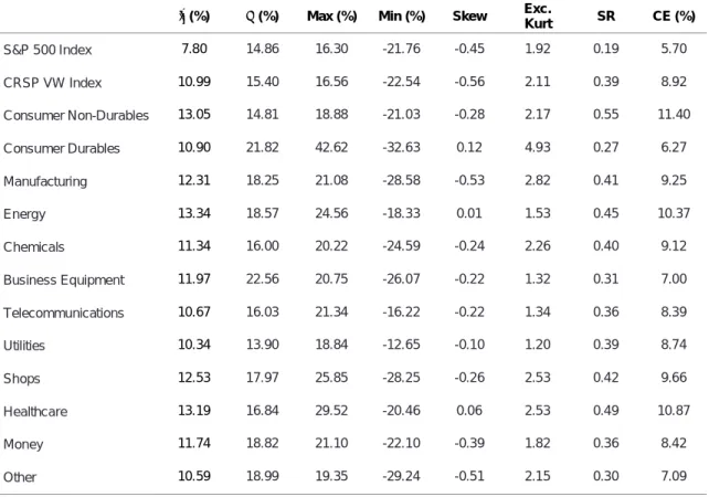
The CRSP index presents a higher Sharpe ratio (0.39) as well as a higher annualized Certainty Equivalent measure (8.92%) when compared to the S&P 500 Index (0.19 and 5.70, respectively). Concerning industry portfolios, we highlight the performance of the Consumer Non-Durables industry, with a Sharpe Ratio of 0.55 and a CE measure of 11.4%.
Table 1. Summary statistics for raw returns
This table presents summary statistics concerning raw returns for the S&P 500 Index, VW industry portfolios from NYSE, AMEX and NASDAQ, as taken from the Kenneth French website, and the VW CRSP index, taken from the WRDS database. The period under analysis comprises January 1963 to June 2014 and excludes months with less than 19 trading days. Thex and the are the annualized mean and standard deviation, respectively, for the return of each index or industry. Skew and Exc. Kurt measure the skewness and excess kurtosis of the series under observation while SR and CE refer to the annualized Sharpe ratio and Certainty equivalent, respectively. We use a power utility function with a coefficient of risk aversion of 2. The average annualized monthly risk-free rate for the period is 4.97%.
x (%) (%) Max (%) Min (%) Skew Exc.
Kurt SR CE (%) S&P 500 Index 7.80 14.86 16.30 -21.76 -0.45 1.92 0.19 5.70 CRSP VW Index 10.99 15.40 16.56 -22.54 -0.56 2.11 0.39 8.92 Consumer Non-Durables 13.05 14.81 18.88 -21.03 -0.28 2.17 0.55 11.40 Consumer Durables 10.90 21.82 42.62 -32.63 0.12 4.93 0.27 6.27 Manufacturing 12.31 18.25 21.08 -28.58 -0.53 2.82 0.41 9.25 Energy 13.34 18.57 24.56 -18.33 0.01 1.53 0.45 10.37 Chemicals 11.34 16.00 20.22 -24.59 -0.24 2.26 0.40 9.12 Business Equipment 11.97 22.56 20.75 -26.07 -0.22 1.32 0.31 7.00 Telecommunications 10.67 16.03 21.34 -16.22 -0.22 1.34 0.36 8.39 Utilities 10.34 13.90 18.84 -12.65 -0.10 1.20 0.39 8.74 Shops 12.53 17.97 25.85 -28.25 -0.26 2.53 0.42 9.66 Healthcare 13.19 16.84 29.52 -20.46 0.06 2.53 0.49 10.87 Money 11.74 18.82 21.10 -22.10 -0.39 1.82 0.36 8.42 Other 10.59 18.99 19.35 -29.24 -0.51 2.15 0.30 7.09 3. Scaled returns
This section presents the methodology used when computing the scaled strategy as well as main results obtained.
3.1. Methodology
The purpose of this strategy is to have an ex-ante constant level of risk over time. With a constant level of volatility, investors are not exposed to crash or fat-tail risk being, therefore, able to maximize expected returns based on a fixed level of volatility over time. The introduction of the Modern Portfolio theory [Markowitz
(1952)] was an advance in the field of constant volatility strategies, since it allowed to compute a portfolio of assets as an equal or value weighted combination of stocks, with the portfolio’s expected return being the weighted combination of their individual returns.
This model allows maximizing a portfolio’s return based on a specific amount of desired portfolio risk or, on the other hand, minimizing the portfolio’s risk taking into consideration a specific level of portfolio return, computed by using different asset weightings. Since the introduction of this model, scaling volatility has been seen in the literature but not with the purpose of the strategy we use in this dissertation. For the computation of the scaled strategy, using stock returns for the previous
month (21 days) we obtain the sum of daily squared returns, where ,
represent the daily raw returns:
To compute the measure of scaled returns, we use the sum of squared returns as obtained from Equation (3), combined with a constant target volatility of 4%
( ):
where , are the raw returns, , ∗ are the scaled returns and
represents the chosen target level of volatility, which for this study corresponds to
= , (3)
the historical monthly level of the S&P 500 index, computed since 1963. 4 Finally, accounts for the return measure as calculated in Equation (3).
3.2. Results
We aim to test if scaling stock returns leads to an increase in Sharpe ratio and to a decrease in tail risk (excess kurtosis). We estimate volatility so as to scale and adjust for the risk exposure present in the S&P 500 index, the CRSP values weighted index and twelve industry portfolios and therefore obtain constant risk over time.
For each month we obtain a measure for scaled returns in which returns are adjusted to account for the same amount of risk using a proxy volatility that corresponds to the monthly historical volatility of S&P 500 (4%), from January 1963 to June 2014.
Table 2 presented below further characterizes the series of scaled returns used in this dissertation where, for each one of the indexes, we present the corresponding annualized measures, where applicable.
4
We also use 2%, 10% and 15% target volatilities, which presented similar results and can be seen in section 5.
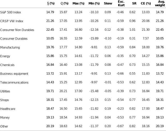
Table 2. Summary statistics for scaled returns
The table below presents summary statistics concerning scaled returns for the S&P 500 Index, the VW CRSP index, taken from the WRDS database and 12 VW industry portfolios from NYSE, AMEX and NASDAQ, as taken from the Kenneth French website. The period under analysis comprises January 1963 to June 2014 and excludes months with less than 19 trading days. Scaled returns are computed using the realized variance for the previous 1 month so as to adjust for the risk exposure of the indexes and the industries, with the benchmark volatility being the monthly historical volatility from S&P500 since 1963, correspondent to 4%. Thex and the are the annualized mean and standard deviation, respectively, for the return of each index or industry. Skew and Exc. Kurt measure the skewness and excess kurtosis of the series under observation while SR and CE refer to the annualized Sharpe ratio and Certainty equivalent, respectively. I use a power utility function with a coefficient of risk aversion of 2. The average annualized monthly risk-free rate for the period is 4.97%. Avg. weight is computed as the target level of volatility divided by the measure.
(%) (%) Max (%) Min (%) Skew Exc.
Kurt SR CE (%)
Avg. weight
S&P 500 Index 14.79 15.87 13.24 -10.10 0.09 -0.46 0.62 13.03 14.79
CRSP VW Index 21.26 17.05 13.95 -10.26 0.11 -0.59 0.96 20.06 21.26
Consumer Non Durables 22.45 17.41 16.80 -12.16 0.12 -0.38 1.01 21.30 22.45
Consumer Durables 10.05 16.55 12.59 -15.89 -0.10 -0.19 0.31 7.57 10.05 Manufacturing 19.76 17.77 14.80 -9.81 0.13 -0.59 0.84 18.00 19.76 Energy 15.86 15.75 14.61 -11.72 0.06 -0.35 0.70 14.27 15.86 Chemicals 16.84 16.40 13.08 -11.79 0.08 -0.47 0.73 15.15 16.84 Business equipment 13.72 15.91 13.17 -9.91 0.13 -0.66 0.55 11.83 13.72 Telecommunications 14.43 15.25 12.95 -9.97 -0.01 -0.53 0.62 12.83 14.43 Utilities 19.71 20.21 17.00 -15.48 -0.05 -0.39 0.73 16.84 19.71 Shops 18.31 17.45 14.76 -12.15 0.15 -0.54 0.77 16.45 18.31 Healthcare 18.47 16.50 15.65 -11.82 0.19 -0.23 0.82 17.00 18.47 Money 19.13 18.54 14.93 -11.94 0.04 -0.53 0.77 16.94 19.13 Other 20.19 18.63 14.62 -11.37 0.20 -0.67 0.82 18.16 20.19
Table 2 strongly supports the hypothesis that risk scaling yields significant advantages, especially for the risk averse investor that wishes to hedge risk in the medium to long term. Taking the raw statistics for the S&P 500 Index, as presented in Table 1, the Sharpe Ratio is of 0.19, while for scaled returns this measure is of 0.62. The Certainty equivalent likewise increases from 5.70% to 13.03%. For the VW CRSP index, scaling results increases the Sharpe ratio from 0.39 to 0.96 and the Certainty equivalent from 8.92 to 20.06. Finally, and
concerning industry portfolios, as observed earlier, the performance of the Consumer Non-Durables industry yielded with raw returns a Sharpe Ratio of 0.55 and a CE measure of 11.4%. By using scaled returns, the Sharpe ratio amounts to 1.01 and the CE totalizes 21.3%.
Barroso & Santa Clara (2013), using momentum, register a variation in the Sharpe Ratio between the raw and the scaled strategy from 0.53 to 0.97, an increase of 83%. In addition, and being highlighted as “the most important gain of risk management” is the decrease in excess kurtosis from 18.24 to 2.68, an indicator of a virtual elimination of momentum crash risk. In real life, eliminating crash risk implies having less volatility in times of significant volatility. For risk averse investors these are good news, since a constant target level of volatility is used and considerable possible future variations and volatility risk are accounted for.
Our results are in line with the results observed in the literature. For S&P 500, excess kurtosis decreases from 1.92 to -0.46, CRSP presents a reduction in excess kurtosis from 2.11 to -0.59 and the Consumer durables industry - the one presenting the highest excess kurtosis figure with raw returns (4.93) - presents a measure of excess kurtosis after computing scaled returns of -0.38, showing as such the benefits of this strategy. This is significantly relevant especially if one considers that during the analysed period there were 7 periods of economic recession versus 8 periods of economic expansion, indicating that the strategy clearly mitigates the excess volatility and uncertainty registered in these periods. As an alternative risk-adjusted performance measure, we compute the alpha from a Carhart (1997) four factor model. In the model, , represents the independent
, = + ( − ) + + + + , (5)
In Equation (5), is the market return at time period t and accounts for the 1 month treasury-bill rate as taken from Kenneth French website, with the difference accounting for market excess return. The factors used represent value-weighted zero investment portfolios, with SMB factor being a proxy for the small versus big capitalization stock strategy. This means that SMB measures the excess return that arises from small capitalization stocks (long) over large capitalization stocks (short). HML, on the other hand, measures the added return brought by high book-to-market stocks in opposition of low book-book-to-market ones. Alpha measures the extra return brought to the investor by opting for the named strategy, with higher alphas being an indicator for adequate and excessive return over risk of the strategy. Table 3 shows these results.
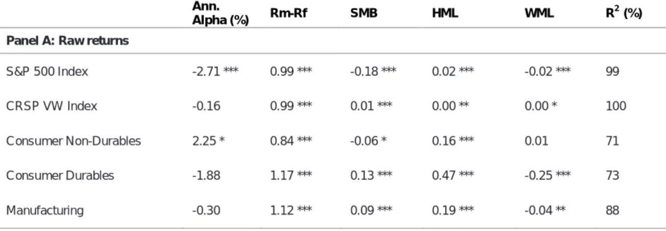
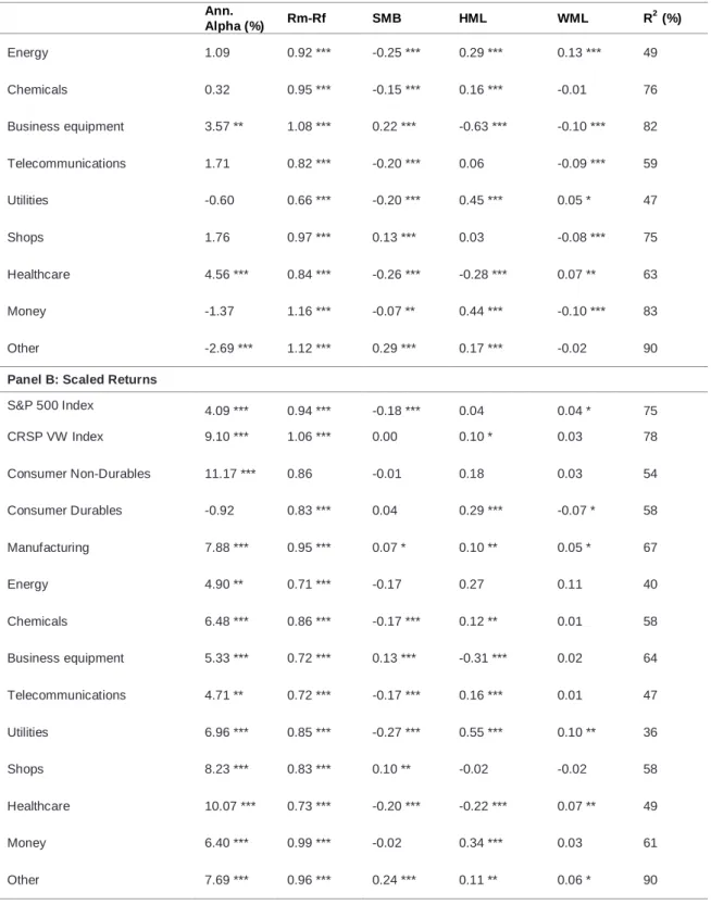
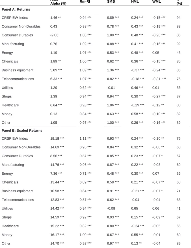
Table 3. Carhart four factor model
The table below includes performance measure statistics for raw (Panel A) and scaled (Panel B) returns for the S&P 500 Index, the VW CRSP index, taken from the WRDS database and 12 VW industry portfolios from NYSE, AMEX and NASDAQ, as taken from the Kenneth French website, concerning the period from January 1963 to June 2014. Scaled returns are computed using the realized variance for the previous 1 month so as to adjust for the risk exposure of the indexes and the industries, with the benchmark volatility being the monthly historical volatility from S&P500 since 1963, correspondent to 4%. The annualized alpha corresponds to the annualized Carhart 4-Factor regression alpha (in percentage). Rm-Rf, SMB, HML, HML and WML are investment strategies benchmarks: market return (risk), small versus large capitalization stocks (size), growth versus value stocks (value) and momentum stocks. The symbols ***, ** and * denote the statistical significance of the coefficients at 1%, 5% and 10% significance level, respectively.
Ann.
Alpha (%) Rm-Rf SMB HML WML R
2
(%)
Panel A: Raw returns
S&P 500 Index -2.71 *** 0.99 *** -0.18 *** 0.02 *** -0.02 *** 99
CRSP VW Index -0.16 0.99 *** 0.01 *** 0.00 ** 0.00 * 100
Consumer Non-Durables 2.25 * 0.84 *** -0.06 * 0.16 *** 0.01 71
Consumer Durables -1.88 1.17 *** 0.13 *** 0.47 *** -0.25 *** 73
Table 3 (continued) Ann. Alpha (%) Rm-Rf SMB HML WML R 2 (%) Energy 1.09 0.92 *** -0.25 *** 0.29 *** 0.13 *** 49 Chemicals 0.32 0.95 *** -0.15 *** 0.16 *** -0.01 76 Business equipment 3.57 ** 1.08 *** 0.22 *** -0.63 *** -0.10 *** 82 Telecommunications 1.71 0.82 *** -0.20 *** 0.06 -0.09 *** 59 Utilities -0.60 0.66 *** -0.20 *** 0.45 *** 0.05 * 47 Shops 1.76 0.97 *** 0.13 *** 0.03 -0.08 *** 75 Healthcare 4.56 *** 0.84 *** -0.26 *** -0.28 *** 0.07 ** 63 Money -1.37 1.16 *** -0.07 ** 0.44 *** -0.10 *** 83 Other -2.69 *** 1.12 *** 0.29 *** 0.17 *** -0.02 90
Panel B: Scaled Returns
S&P 500 Index 4.09 *** 0.94 *** -0.18 *** 0.04 0.04 * 75 CRSP VW Index 9.10 *** 1.06 *** 0.00 0.10 * 0.03 78 Consumer Non-Durables 11.17 *** 0.86 -0.01 0.18 0.03 54 Consumer Durables -0.92 0.83 *** 0.04 0.29 *** -0.07 * 58 Manufacturing 7.88 *** 0.95 *** 0.07 * 0.10 ** 0.05 * 67 Energy 4.90 ** 0.71 *** -0.17 0.27 0.11 40 Chemicals 6.48 *** 0.86 *** -0.17 *** 0.12 ** 0.01 58 Business equipment 5.33 *** 0.72 *** 0.13 *** -0.31 *** 0.02 64 Telecommunications 4.71 ** 0.72 *** -0.17 *** 0.16 *** 0.01 47 Utilities 6.96 *** 0.85 *** -0.27 *** 0.55 *** 0.10 ** 36 Shops 8.23 *** 0.83 *** 0.10 ** -0.02 -0.02 58 Healthcare 10.07 *** 0.73 *** -0.20 *** -0.22 *** 0.07 ** 49 Money 6.40 *** 0.99 *** -0.02 0.34 *** 0.03 61 Other 7.69 *** 0.96 *** 0.24 *** 0.11 ** 0.06 * 90
Annualized alpha for the S&P 500 Index increases from -2.71% for raw returns to 4.09% with constant volatility over time. These results are consistent over the CRSP index (annualized alpha increases from -0.16 to 9.10) and the 12 industry
portfolios. It should also be noted that scaled returns present higher levels of statistical significance when compared to raw returns and that both raw and scaled returns present a quite large explanatory power.
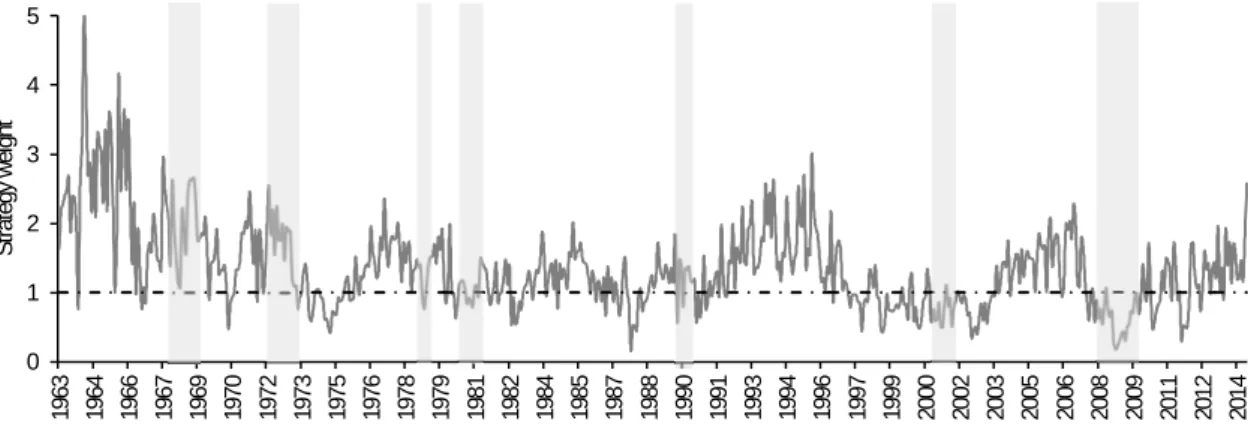
Another important component of the scaled strategy is strategy weights over time. Figure 1 presents the weights of the scaled volatility strategy over time for the S&P index, computed as the ratio between the chosen level of target volatility and the monthly volatility computed from Equation (3), using the sum of daily squared returns. Equation (6) below clarifies the computation of this indicator.
Stock return weights range from 0.16 to 5.10. As expected, lowest strategy weights correspond to periods of high volatility and overall economic recession. The average strategy weight for recession periods is 0.85 while for expansion periods it accounts for 1.46. The lowest weight for S&P 500 was registered in October 1987, the Black Monday, when the registered index return was of -22%. Following this period, October 2008 was the month which registered the lowest index returns, where the strategy weights corresponded to 0.18.
Concerning expansion periods, the period of 1963-1969 presents considerable higher weights, varying from 5.10 in February 1964 to 4.16 in August 1965. June 2014, the last analysed month in our sample, presents a weight of 2.57. Shaded areas in Figure 1 below represent recession periods according to the National Bureau of Economic research.
Figure 1. Strategy weights
The figure below presents the strategy weights as calculated from Equations (3) and (4), for the scaled returns of the S&P index. The dotted line represents the weight benchmark of 1. Scaled returns are computed using historical returns for the previous month with a target volatility corresponding to the monthly historical volatility of the S&P index, since 1963, as the measure for risk exposure. Shaded regions represent the National Bureau of Economic Research recession periods.
4. Industry momentum
Momentum strategies have been extensively studied in past literature. Winners minus losers’ strategies using returns from the previous 6 to 12 months yield Sharpe ratios higher than the markets and statistically significant alphas across several asset classes, markets and periods of time. Jegadeesh & Titman (1993, 2001) first document the success of momentum strategies applied to US data, from 1965 to 1989 and in a later study from 1990 to 1998. They find that previous winners outperform previous losers by 1.49 percent a month and show that, from 1927 until 2001, momentum had a monthly excess return of 1.75 percent controlling for the Fama-French factors. Asness (1995) shows that the strategy is more efficient if based on the most recent past month. Rouwenhorst (1998,1999) presents very similar results for the european and emerging markets, respectively, and ssimilar evidence of the success of the strategy has been shown when applied to the futures markets [Moskowitz et al. (2012)], commodities [Erb & Harvey
0 1 2 3 4 5 19 63 19 64 19 66 19 67 19 69 19 70 19 72 19 73 19 75 19 76 19 78 19 79 19 81 19 82 19 84 19 85 19 87 19 88 19 90 19 91 19 93 19 94 19 96 19 97 19 99 20 00 20 02 20 03 20 05 20 06 20 08 20 09 20 11 20 12 20 14 St ra te gy w ei gh t
(2006)], currency markets [Okunev & White (2003) and Menkhof et al. (2012)], industry portfolios [(Moskowitz & Grinblatt (1999)] or bonds [Asness et al. (2013)]. Grundy & Martin (2001) and Daniel & Moskowitz (2012) focus on the time-varying systematic risk on momentum, rather than its specific risk as Barroso & Santa Clara (2013). They show that specific risk is more predictable than the first, yielding an out of sample R-Squared of 47 percent on opposition to 21 percent if using time-varying systematic risk, enabling therefore investors to manage risk while avoiding forward-looking bias.
Barroso & Santa-Clara (2013) explore momentum strategies in the sense that high Sharpe ratios are also accompanied by occasional large crashes, as also explored by Kent & Moskowitz (2013). The authors mention particular periods of recessions such as 1932 (the WML strategy yielded a -91.59 percent return in two months) and 2009 (a percent return of -73.42 percent in 3 months), where the large returns from momentum do not offset for the significant losses incurred in these periods, even for investors which undertake considerable levels of risk aversion. They find that after scaling this risk, not only the Sharpe ratio of the strategy significantly increases but crashes are nearly eliminated, with excess excess kurtosis decreasing from 18.24 to 2.68.
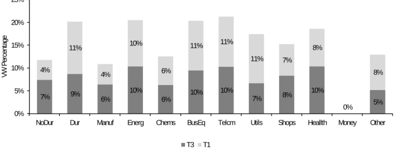
In this section we present scaling volatility strategies applied to momentum. We take cumulative returns, from the past 12 months, and apply a rolling window. Afterwards, we sort the industries in ascending order according to these cumulative excess returns and go long (short) the top (bottom) tercile of these sorted industries. For a sample composed of VW industry returns, figure 2 shows
7% 9% 6% 10% 6% 10% 10% 7% 8% 10% 0% 5% 4% 11% 4% 10% 6% 11% 11% 11% 7% 8% 8% 0% 5% 10% 15% 20% 25%
NoDur Dur Manuf Energ Chems BusEq Telcm Utils Shops Heallth Money Other
VW Pe rc en ta ge T3 T1
the contribution over time of each industry, measured as percentage, for either portfolio T3 (winner) or T1 (loser).
Figure 2. Momentum weights
The figure below presents the relative frequency for which each industry was a winner (T3) or a loser (T1). For each month we compute which industries were the top 3 winners and 3 losers and calculate its frequency, based on the total number of months. Returns were calculated as weights for each strategy, concerning the long and short legs. For each month the 3 winner and 3 loser industries were calculated using the cumulative returns from the past 12 months from industry portfolios. The period under analysis comprises December 1963 until June 2014 and excludes months with less than 19 trading days.
So as to compute a momentum strategy performance measure, we compute, for each month and for each individual portfolio, the average of the 3 winner industries (T3), with T1 being the average of the 3 loser industries. Additionally, we also present summary statistics concerning momentum strategies. For each strategy – MOM 1 Raw, MOM 1 Scaled and MOM 2 we present measures of performance evaluation.
Concerning the computation of each strategy, MOM 1 Raw concerns the T3-T1 portfolio statistic, computed using raw returns, while for the computation of the measure of MOM 1 Scaled were used MOM 1 Raw, the target volatility of 4%, as used previously, and the sum of daily squared returns. Finally, MOM 2
corresponds to the scaled MOM 1 indicator, computed by using the scaled T3-T1 return portfolios, the sum of daily squared returns and the target level of volatility. Table 4 presents the results of the scaled strategy applied to momentum portfolios.
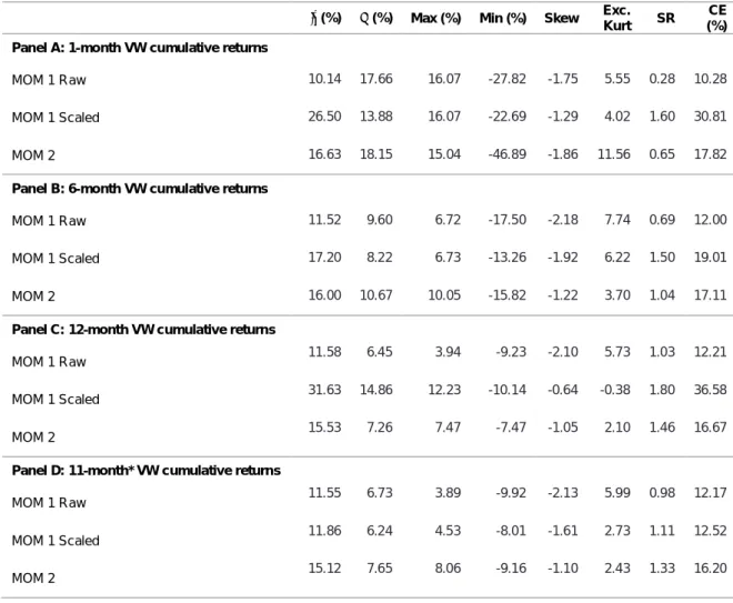
Table 4. Momentum strategies
The table below presents the results for momentum monthly strategies based on cumulative returns from the past 1, 6, 11 and 12 months from industry portfolios. T3 is the average of the 3 winner industries while T1 is the average of the 3 loser industries. MOM 1 Raw is the T3-T1 portfolio measure, computed with raw returns, while MOM 1 Scaled uses MOM 1 Raw, the target volatility of 4% and the sum of daily squared returns to compute the scaled measure. Finally, MOM 2 corresponds to the scaled MOM 1 indicator, calculated using the scaled T3-T1 return portfolios, the sum of daily squared returns and the target level of volatility. The period under analysis comprises cumulative returns starting as of December 1963 until June 2014 and excludes months with less than 19 trading days. The x and the are the annualized mean and standard deviation, respectively, for the return or scaled return of each strategy. Skew and Exc. Kurt measure the skewness and excess kurtosis of the series under observation while SR and CE refer to the annualized Sharpe ratio and Certainty equivalent, respectively. We use a power utility function with a coefficient of risk aversion of 2. The average annualized monthly risk-free rate for the period is 4.97%.
(%) (%) Max (%) Min (%) Skew Exc. Kurt SR
CE (%) Panel A: 1-month VW cumulative returns
MOM 1 Raw 10.14 17.66 16.07 -27.82 -1.75 5.55 0.28 10.28
MOM 1 Scaled 26.50 13.88 16.07 -22.69 -1.29 4.02 1.60 30.81
MOM 2 16.63 18.15 15.04 -46.89 -1.86 11.56 0.65 17.82
Panel B: 6-month VW cumulative returns
MOM 1 Raw 11.52 9.60 6.72 -17.50 -2.18 7.74 0.69 12.00
MOM 1 Scaled 17.20 8.22 6.73 -13.26 -1.92 6.22 1.50 19.01
MOM 2 16.00 10.67 10.05 -15.82 -1.22 3.70 1.04 17.11
Panel C: 12-month VW cumulative returns
MOM 1 Raw 11.58 6.45 3.94 -9.23 -2.10 5.73 1.03 12.21
MOM 1 Scaled 31.63 14.86 12.23 -10.14 -0.64 -0.38 1.80 36.58
MOM 2 15.53 7.26 7.47 -7.47 -1.05 2.10 1.46 16.67
Panel D: 11-month* VW cumulative returns
MOM 1 Raw 11.55 6.73 3.89 -9.92 -2.13 5.99 0.98 12.17
MOM 1 Scaled 11.86 6.24 4.53 -8.01 -1.61 2.73 1.11 12.52
MOM 2 15.12 7.65 8.06 -9.16 -1.10 2.43 1.33 16.20
When analysing Table 4, and having computed the measures for different cumulative returns rolling window periods, it is observable that results are robust
across all the analysed cumulative return windows and periods. The Sharpe Ratios consistently improves when using the scaled versus the raw returns, as well as the Certainty Equivalent. In addition, the results are consistent over MOM 1 Scaled and MOM 2, meaning that despite the different calculation methods for the scaled strategy, the results are consistent and overall higher than raw returns. As seen previously in the literature, it should also be noticed the overall reduction in excess kurtosis as an indication that crash risk is reduced and hence the investor is successfully being able to hedge its risk over time.
5. Robustness tests
This section tests the robustness of the results achieved with the volatility scaling strategy applied for stock returns. We test for expansion vs. recession periods as a way of showing the effects of the reduction of crash risk we achieved earlier in this study and to further clarify on the behaviour of the strategy under different market conditions. We also run a winners-minus-losers strategy on raw and scaled returns to test for consistency over different asset classes and to further examine the consistency of the results with the momentum strategies analysed in the literature. Finally, we test the behaviour of the strategy under different target volatility levels.
5.1. Equally weighted data
Table 5 presents results obtained for the methodology described throughout this paper for raw returns and scaled returns computed using a measure of equally weighted returns for both S&P 500 and the CRSP index.
Concerning raw returns, it should be noted that the average for EW returns is higher (15.07%) when compared to the VW measure (11.83%), as well as the corresponding average annualized Sharpe Ratio (0.48 for EW returns versus a measure of 0.39 when using VW returns). This goes in line with the rationale behind each method’s calculations since equally-weighted returns give a similar weight to every stock in the index, meaning that for instance small caps and riskier stocks have the same weight as a stock from a long-term, low volatile, already established company.
The results obtained are consistent over the different industries being used in our sample, where we highlight the range of Sharpe ratio obtained when using scaled returns, with the measure varying from 0.72 (Energy) to 1.16 (Money).
Table 5. Summary statistics for equally weighted data
The table below presents summary statistics concerning raw and scaled returns for the EW industry portfolios from NYSE, AMEX and NASDAQ, as taken from the Kenneth French website, and the EW CRSP index, taken from the WRDS database. EW1 represents the aggregated industry equally weighted strategy and EW2 is the scaled EW1 indicator. The period under analysis comprises January 1963 to June 2014 and excludes months with less than 19 trading days. Scaled returns are computed using the realized variance for the previous 1 month so as to adjust for the risk exposure of the indexes and the industries, with the benchmark volatility being the monthly historical volatility from S&P500 since 1963, correspondent to 4%. Thex and the are the annualized mean and standard deviation, respectively, for the return of each index or industry. Skew and Exc. Kurt measure the skewness and excess kurtosis of the series under observation while SR and CE refer to the annualized Sharpe ratio and Certainty equivalent, respectively. I use a power utility function with a coefficient of risk aversion of 2. The average annualized monthly risk-free rate for the period is 4.97%.
x (%) (%) Max (%) Min (%) Skew Exc.
Kurt SR CE (%) Panel A: Returns CRSP Index 14.50 19.52 29.93 -27.22 -0.20 3.03 0.49 11.17 Consumer Non-Durables 13.48 18.76 28.75 -27.93 -0.11 4.23 0.46 10.38 Consumer Durables 12.93 23.62 38.31 -31.56 0.04 4.27 0.33 7.51 Manufacturing 15.17 20.94 28.29 -29.86 -0.31 3.16 0.49 11.21 Energy 16.91 26.23 28.34 -32.66 -0.13 1.95 0.46 10.36 Chemicals 15.23 19.62 25.93 -29.57 -0.46 3.41 0.53 11.86 Business equipment 17.08 29.34 47.17 -31.73 0.31 2.69 0.42 8.90 Telecommunications 16.88 25.59 52.81 -27.39 0.36 5.25 0.47 10.88 Utilities 12.24 12.29 22.76 -13.07 0.11 2.95 0.60 11.29
Table 5 (continued)
x (%) (%) Max (%) Min (%) Skew Exc.
Kurt SR CE (%) Shops 14.06 21.49 34.84 -29.64 0.05 4.19 0.43 9.82 Healthcare 18.10 24.71 42.99 -32.67 0.23 3.05 0.53 12.72 Money 13.98 17.41 28.77 -21.28 -0.14 3.10 0.52 11.48 Other 14.77 21.66 29.02 -30.78 -0.20 2.65 0.46 10.46 EW1 14.98 19.70 28.52 -27.21 -0.28 2.92 0.51 11.78
Panel B: Scaled Returns
CRSP Index 32.06 23.66 17.97 -11.77 0.10 -0.86 1.15 30.14 Consumer Non-Durables 28.67 22.52 17.64 -11.99 0.11 -0.72 1.05 26.45 Consumer Durables 21.88 21.92 17.27 -12.09 0.16 -0.72 0.77 18.62 Manufacturing 28.97 23.01 18.14 -11.92 0.10 -0.84 1.05 26.60 Energy 20.11 21.20 16.85 -15.58 -0.02 -0.37 0.72 16.84 Chemicals 26.02 19.83 17.62 -11.62 0.10 -0.59 1.06 24.58 Business equipment 22.23 22.87 17.94 -11.13 0.17 -0.79 0.76 18.54 Telecommunications 24.39 21.25 17.58 -11.89 0.05 -0.80 0.92 21.90 Utilities 28.45 21.52 17.77 -15.91 -0.05 -0.52 1.09 26.69 Shops 27.82 23.80 18.23 -14.31 0.13 -0.80 0.96 24.75 Healthcare 26.03 22.62 18.40 -11.27 0.16 -0.86 0.93 23.21 Money 31.72 23.09 18.34 -13.37 0.02 -0.65 1.16 29.99 Other 28.44 23.56 20.25 -12.81 0.18 -0.71 1.00 25.66 EW1 25.53 19.75 16.53 -11.22 0.08 -0.71 1.04 24.02 EW2 24.42 19.32 16.50 -10.88 0.09 -0.70 1.01 22.86
We present in Table 6, as an additional measure for performance evaluation, the Carhart four factor model statistics. Again, we highlight not only more robust results for EW returns when compared to VW returns but also how for the EW indexes the annualized alpha for the VW CRSP index increases from 1.46 to 19.18 when using a constant level of target volatility over time.
Table 6. Carhart four factor model for EW returns
The table below includes performance measure statistics for raw (Panel A) and scaled (Panel B) returns for S&P 500, the EW CRSP index and 12 EW industry portfolios, concerning the period from January 1963 to June 2014. The annualized alpha corresponds to the annualized Carhart 4-Factor regression alpha (in percentage). Rm-Rf, SMB, HML and WML are investment strategies benchmarks: market return (risk), small versus large capitalization stocks (size), growth versus value stocks (value) and momentum stocks. The symbols ***, ** and * denote the statistical significance of the coefficients at 1%, 5% and 10% significance level, respectively.
Ann. Alpha (%) Rm-Rf SMB HML WML R2 (%) Panel A: Returns CRSP EW Index 1.46 ** 0.94 *** 0.89 *** 0.24 *** -0.15 *** 94 Consumer Non-Durables 0.43 0.88 *** 0.78 *** 0.43 *** -0.19 *** 88 Consumer Durables -2.06 1.08 *** 1.00 *** 0.48 *** -0.23 *** 86 Manufacturing 0.76 1.02 *** 0.88 *** 0.41 *** -0.16 *** 92 Energy 1.19 1.07 *** 0.53 *** 0.48 *** 0.05 46 Chemicals 1.89 ** 1.00 *** 0.62 *** 0.36 *** -0.15 *** 85 Business equipment 5.09 *** 1.09 *** 1.36 *** -0.37 *** -0.24 *** 86 Telecommunications 6.33 *** 1.07 *** 0.82 *** -0.18 *** -0.31 *** 76 Utilities 1.29 0.62 *** -0.01 0.46 *** 0.01 56 Shops 1.39 0.94 *** 0.94 *** 0.30 *** -0.27 *** 87 Healthcare 6.64 *** 0.93 *** 1.06 *** -0.29 *** -0.12 ** 80 Money 0.13 0.84 *** 0.63 *** 0.58 *** -0.10 *** 82 Other 1.05 0.97 *** 1.00 *** 0.26 *** -0.16 *** 89
Panel B: Scaled Returns
CRSP EW Index 19.18 *** 1.11 *** 0.93 *** 0.24 *** -0.10 ** 75 Consumer Non-Durables 14.69 *** 0.93 *** 0.84 *** 0.32 *** -0.08 ** 68 Consumer Durables 8.56 *** 0.87 *** 0.85 *** 0.23 *** -0.07 * 67 Manufacturing 14.76 *** 0.96 *** 0.87 *** 0.22 *** -0.03 69 Energy 7.36 *** 0.71 *** 0.48 *** 0.30 *** 0.07 36 Chemicals 13.44 *** 0.89 *** 0.58 *** 0.21 *** -0.07 ** 68 Business equipment 10.98 *** 0.84 *** 0.91 *** -0.21 *** -0.07 * 71 Telecommunications 12.83 *** 0.87 *** 0.62 *** -0.04 -0.04 63 Utilities 14.42 *** 0.94 *** -0.08 0.65 0.06 41 Shops 14.59 *** 0.92 *** 0.93 *** 0.15 *** -0.09 ** 67 Healthcare 15.22 *** 0.82 *** 0.80 *** -0.24 *** -0.05 65 Money 16.17 *** 1.00 *** 0.67 *** 0.55 *** -0.01 60 Other 14.70 *** 0.92 *** 0.97 *** 0.13 ** -0.04 89
5.2. T-regulation
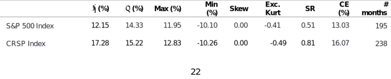
As a way of further testing the behaviour of our strategy over time, we have performed a T-regulation exercise over the strategy weights of the scaled strategy. As mentioned in section 3.2, the scaled strategy’s average weights range from 0.16 to 5.10, with lower weights corresponding to overall recessive economic periods with high volatility. Having a majority number of months corresponding to expansion periods, it should not come as a surprise that higher weights have a higher influence on the behaviour of weights over time. In this section we perform a T-regulation analysis, where we restrict the strategy’s weight to 1.5 if it is higher than this value. Table 7 presents the main results. Limiting the strategy’s weight does not change the overall results over time. S&P 500 presents a Sharpe ratio of 0.62 with a calculation base of unrestricted returns, while the restricted-return Sharpe ratio varies to 0.51. Concerning the CRSP index, the difference is from 0.96 in the unrestricted sample to 0.81 in the restricted sample. Even though the Certainty equivalence measures have decreased slightly on the restricted sample, we do not consider this to invalidate the overall results of our strategy.
Table 7. Scaled returns with T-Regulation
The table below presents summary statistics concerning scaled returns for the S&P 500 Index, VW industry portfolios and the VW CRSP index. For the weights of the computation of the scaled returns, we impose a restriction where if it exceeds 1.5 it remains as such. The column ‘# months’ presents the number of months which have exceeded a weight of 1.5 and where the restriction has been imposed. The period under analysis comprises January 1963 to June 2014 and excludes months with less than 19 trading days. The x and the are the are the annualized mean and standard deviation, respectively while Skew and Exc. Kurt measure the skewness and excess kurtosis of the series under observation. SR and CE refer to the annualized Sharpe ratio and Certainty equivalent, respectively. We use a power utility function with a coefficient of risk aversion of 2. The average annualized monthly risk-free rate for the period is 4.97%.
x (%) (%) Max (%) Min(%) Skew Exc.Kurt SR (%)CE months#
S&P 500 Index 12.15 14.33 11.95 -10.10 0.00 -0.41 0.51 13.03 195
Table 7 (continued)
(%) (%) Max (%) Min (%) Skew Exc.
Kurt SR CE (%) Ann. Alpha (%) Consumer Non-Durables 15.43 17.38 15.97 -21.47 -0.44 1.51 0.60 13.07 270 Consumer Durables 9.39 18.59 20.64 -21.17 -0.13 0.99 0.24 6.07 61 Manufacturing 13.85 18.94 20.80 -28.34 -0.25 1.94 0.47 10.71 162 Energy 13.16 16.70 20.37 -13.98 0.17 0.85 0.49 10.92 110 Chemicals 13.56 17.02 21.41 -20.60 0.07 1.21 0.51 11.23 170 Business Equipments 10.60 17.36 20.98 -20.28 0.11 0.79 0.33 7.89 35 Telecommunications 12.68 15.73 14.72 -12.31 -0.07 0.08 0.49 10.71 158 Utilities 14.17 17.43 19.28 -18.29 0.02 0.73 0.53 11.75 355 Shops 13.43 19.07 17.78 -25.56 -0.28 1.86 0.45 10.18 150 Healthcare 13.96 17.40 17.54 -19.05 -0.09 0.74 0.52 11.50 123 Money 13.36 19.24 18.43 -26.31 -0.37 1.47 0.44 10.02 194 Other 18.06 17.62 13.82 -11.37 0.15 -0.63 0.75 16.10 159 5.3. Periods
We test for the robustness of the strategy over expansion and recession periods, by taking the definition of the US economic periods out of the National Bureau of Economic Research. 5 From the whole sample of monthly returns, we separately filter for expansion and recession periods and compute raw and scaled returns as well as the remaining statistics presented earlier in this study. From 1963 until 2014, we identify 7 recession periods consisting of 83 months and 6 expansion periods corresponding to the remaining months. Please refer to Figure 1 where we present a graphical representation of recession and expansion NBER periods, included in the graph as shaded areas. Using the identified recession and
5
expansion periods, we study the effects of the economic cycles for S&P 500 and the CRSP index on raw and scaled returns. Please refer to table 8 below.6
Table 8. Summary statistics for different periods
The table below presents summary statistics concerning raw and scaled returns for the S&P 500 Index and the VW CRSP index taken from the WRDS database. The period under analysis comprises January 1963 to June 2014 and is divided into (i) two halves and (ii) recession and expansion periods, taken from NBER. Scaled returns are computed using the realized variance for the previous month so as to adjust for the risk exposure of the indexes and the industries, with the benchmark volatility being the monthly historical volatility from S&P500 since 1963, correspondent to 4%. The x and the are the annualized mean and standard deviation. Skew and Exc. Kurt measure the skewness and excess kurtosis of the series under observation while SR and CE refer to the annualized Sharpe ratio and Certainty equivalent, respectively. We use a power utility function with a coefficient of risk aversion of 2. The average annualized monthly risk-free rate for the period is 4.97%.
(%) (%) Max (%) Min (%) Skew Exc.
Kurt SR CE (%)
Ann. Alpha
(%)
Panel A: Raw returns
1st half S&P 500 Index 6.84 15.14 16.30 -21.76 -0.30 2.56 0.02 4.61 -3.46 *** CRSP VW 10.98 15.77 16.56 -22.54 -0.39 2.60 0.28 8.80 -0.32 2nd half S&P 500 Index 8.90 14.59 11.16 -16.94 -0.62 1.24 0.02 4.61 -1.93 *** CRSP VW 11.00 15.01 11.40 -18.46 -0.75 1.56 0.52 8.80 3.39 *** Recession periods S&P 500 Index 1.62 21.66 16.30 -16.94 0.04 -0.12 -0.52 -2.49 -3.58 *** CRSP VW 4.99 21.81 16.56 -12.02 0.21 -0.35 -0.14 2.80 -0.18 Expansion periods S&P 500 Index 8.97 13.42 13.18 -21.76 -0.55 2.83 0.28 7.37 -2.49 *** CRSP VW 12.33 13.79 12.85 -22.54 -0.73 3.14 0.51 10.89 -0.06
Panel B: Scaled Returns
1st half S&P 500 Index 13.18 17.67 13.24 -10.10 0.12 -0.64 0.38 10.59 2.09 CRSP VW 35.98 26.26 18.08 -11.84 0.07 -1.03 1.12 19.64 19.62 *** 2nd half S&P 500 Index 16.55 13.84 11.95 -7.92 0.09 -0.48 0.48 15.70 6.47 *** 6
We also compute recession and expansion statistics for the individual industry portfolios. The results are consistent with the ones presented for the remaining indexes but are excluded for the sake of simplicity.
Table 8 (continued)
(%) (%) Max (%) Min (%) Skew Exc.
Kurt SR CE (%) Ann. Alpha (%) CRSP VW 28.63 21.02 16.80 -11.31 0.07 -0.80 1.40 27.24 17.00 *** Recession periods S&P 500 Index -0.68 15.36 8.36 -10.10 0.03 -0.89 -0.47 -2.97 -1.75 CRSP VW 4.75 17.55 10.91 -11.31 -0.07 -0.74 -0.18 11.17 1.46 Expansion periods S&P 500 Index 16.21 16.09 13.24 -9.83 0.13 -0.42 0.68 14.55 3.38 *** CRSP VW 21.89 16.59 15.57 -10.61 0.11 -0.35 1.00 20.98 3.52 ***
One of the striking conclusions arising from Table 8 is the fact that across all periods, the Sharpe ratio and the annualized CE increase when comparing scaled to raw returns. Additionally, the annualized alpha likewise improves when applying a target volatility strategy across all sub samples. During recession periods, we highlight the slight decrease of the SR in the S&P 500 Index when comparing raw and scaled returns, from -0.52 to -0.47 and the improve concerning the annualized alpha, from -3.58 to -1.75. The same conclusions arise from the computations using the CRSP VW Index, where during recession periods annualized alpha increases from -0.18 to 1.46. Concerning expansion periods, we highlight the Sharpe ratio increase, for the S&P 500 Index, from 0.28 using raw returns to 0.68 with scaled returns.
The same trend is verified for CRSP, where this indicator increases from 0.51 to 1. Also, it should be mentioned the increase in annualized alpha, from -2.49 to 3.38 (S&P 500) and from -0.06 to 3.52 (CRSP) should be noted. We have also computed raw versus scaled statistics with the raw sample divided in half and have arisen to similar results.
5.4. Target volatility
Finally, the robustness of results was tested for different levels of target volatility. Results with target volatility of 4%, as used in the remainder of this study, yield annualized returns of 14.79%, an annualized Sharpe ratio measure of 0.62 and a Certainty equivalent of 13.03%. Table 9 summarizes results obtained for different target volatility measures. Results are consistent across different choices for target volatility both for S&P 500 and the CRSP value-weighted index.
Table 9. Summary statistics with different target volatilities
The table below presents summary statistics concerning raw and scaled returns for the S&P 500 Index and the VW CRSP Index, taken from the WRDS database. The period under analysis comprises January 1963 to June 2014. Scaled returns are computed using the realized variance for the previous month so as to adjust for the risk exposure of the indexes and the industries with the benchmark volatilities being 2%, 10%,15% and 20% as opposed to the 4% level used throughout the dissertation (the monthly historical volatility from S&P500 since 1963). Thex and the are the annualized mean and standard deviation, respectively, for the return or scaled return of each index or strategy. Skew and Kurt measure the skewness and excess kurtosis of the series under observation while SR and CE refer to the annualized Sharpe ratio and Certainty equivalent, respectively. I use a power utility function with a coefficient of risk aversion of 2. The average annualized monthly risk-free rate for the period is 4.97%.
(%) (%) Max (%) Min (%) Skew Exc.
Kurt SR CE (%) Ann. Alpha (%) Panel A: 2% Volatility S&P 500 Index 7.47 9.74 8.35 -6.63 -0.09 -0.42 0.26 5.54 -1.09 *** CRSP VW 10.53 10.25 8.56 -7.22 -0.14 -0.41 0.55 9.60 1.50 *** Panel B: 10% Volatility S&P 500 Index 16.70 21.79 18.68 -14.83 -0.09 -0.42 0.54 9.52 3.63 *** CRSP VW 14.20 17.74 17.34 -16.14 -0.25 0.55 0.52 11.04 2.39 *** Panel C: 15% Volatility S&P 500 Index 20.46 26.69 22.87 -18.17 -0.09 -0.42 0.58 10.15 5.54 *** CRSP VW 13.90 18.36 20.28 -19.33 -0.32 0.96 0.49 10.77 1.84 *** Panel D: 20% Volatility S&P 500 Index 23.62 30.81 26.41 -20.98 -0.09 -0.42 0.61 10.21 7.16 *** CRSP VW 13.74 18.52 20.28 -20.96 -0.37 1.16 0.48 10.58 1.52 ***
6. Conclusions
This thesis presents evidence of the success of volatility scaling strategies. I use stock returns from the S&P 500, the CRSP index and 12 industry portfolios for a period ranging from January 1963 to June 2014 to test for the success of scaled volatility strategies over time.
We extend the existing literature by developing a constant volatility strategy where risk is kept constant throughout time so as to control future volatility fluctuations and the negative consequences of tail risk. We manage to show that managing volatility risk virtually eliminates exposure to crashes and increases the Sharpe ratio and the Certainty equivalent of the strategies substantially. Across different time periods, different indexes calculation methodologies and by restricting the strategy’s weights to dilute the effect of economic expansions, the strategy proves to be robust and allows to show that scaling for risk and keeping a constant level of volatility over time which corresponds to the historical volatility of S&P 500 -dramatically reduces the investors’ medium to long term portfolio risk.
We also find a considerably decrease of excess kurtosis when using scaled returns and find that keeping a constant target level of volatility over time contributes to a higher performance and a better fit between the strategy’s risk and return, yielding as so considerable higher profits for the investor, reflected both in the Sharpe ratio, Certainty equivalence and annualized alpha performance measures.
The contribution of this thesis could, however, be complemented by further research such as the inclusion of transaction costs for stock return scaled volatility.
7. References
Asness, C. S. 1995. The power of past stock returns to explain future stock returns. Working
paper series.
Asness, C. S., Moskowitz, T. J. & Pedersen, L. H., 2013. Value and momentum everywhere.
The Journal of Finance. Volume 68, Issue 3, pp. 929-985.
Baltas, A. & Kosowski, R., 2013. Momentum strategies in futures markets and trend-following Funds. Working paper series.
Barroso, P. & Santa-Clara, P., 2013. Momentum has its moments. Journal of Financial
Economics (forthcoming).
Erb, C. & Harvey, C. R., 2006. The strategic and tactical value of commodity futures. Financial
Analysts Journal. Volume 62, pp. 69-97.
Fama, E., 1970. Efficient capital markets: A review of theory and empirical work. The Journal of
Finance. Volume 25, Issue 2, pp. 383-417.
Ferreira, M. & Santa-Clara, P., 2011. Forecasting stock market returns: The sum of the parts is more than the whole. Journal of Financial Economics. Volume 100, pp. 514-537.
French, K. R. & Roll, R., 1986. Stock return variances: The arrival of information and the reaction of traders. Journal of Financial Economics. Volume 17, pp. 5-26.
Grinblatt, M. & Titman, S., 1989. Mutual fund performance: An analysis of quarterly portfolio holdings. Journal of Business, Volume 62, pp. 394-415.
Grinblatt, M. & Titman, S., 1993. Performance measurement without benchmarks: An examination of mutual fund returns. Journal of Business. Volume 66, pp. 47-68.
Hou, K., Karolyi, G. A. & Kho, B. C., 2011. What factors drive global stock returns?. The Review
of Financial Studies. pp. 2527-2574.
Hou, K. & Robinson, D. T., 2006. Industry concentration and average stock returns. The Journal
of Finance. Volume 61, Issue 4, pp. 1927-1956.
Jegadeesh, N. & Titman, S., 1993. Returns to buying winners and selling losers: Implications for stock market efficiency. The Journal of Finance. Volume 48, pp. 65-91.
Jegadeesh, N. & Titman, S., 2001. Momentum. Working paper series. Kent, D. & Moskowitz, T., 2013. Momentum crashes. Working paper series.
Moskowitz, T., Ooi, Y. & Pedersen, L., 2012. Time series momentum. Journal of Financial
Economics. Volume 104, pp. 228-250.
Rouwenhorst, K. G., 1998. International momentum strategies. The Journal of Finance. Volume
53, Issue 1, pp. 267-282.
Rouwenhorst, K. G., 1999. Local return factors and turnover in emerging stock markets. The
Journal of Finance. Volume 54, Issue 4, pp. 1439-1464.
Schwert, G. W., 1989. Why does stock market volatility change over time? The Journal of
Finance. Volume 44, Issue 5, pp. 1115-1153.
Sharpe, W. F., 1964. Capital asset prices: A theory of market equilibrium under conditions of risk. The Journal of Finance. Volume 19, Issue 3, pp. 425 - 442.