Equity Valuation Using Accounting Numbers
High vs. Low Proportion of Intangibles in Firms
Gonçalo Morais Sarmento
Dissertation submitted in partial fulfilment of requirements for the degree of International MSc in Management at Católica Lisbon School of Business and Economics and MSc in Finance
2
Abstract
The shift to a new economy places on intangible assets an indispensable instrument to preserve the competitive positions of firms and their value creation process. Due to their nature being difficult to define, the wealth created by intangible assets may not be fully captured by the current accounting standards which are based on limited recognition criteria. This paper sheds light on the importance of accounting information for valuation and offers a study of how equity valuation models perform in measuring the value of firms with high and low proportions of intangibles. To this end, a comprehensive review of literature relevant to the matter of equity valuation using accounting numbers is offered followed by the results of the analyses performed to a large and a small samples of US and UK publicly traded firms. It is found that the separation of the samples into firms with high and low proportions of intangibles produces in some cases evident differences whilst in others there are no conclusive disparities. The RIVM is proven to provide superior valuation performance when compared to the P/E multiple and some tendencies in varying approaches to firm valuation by analysts, according to the extent of intangible asset proportion, are observed yet not confirmed.
Key words: Equity Valuation, Firm Valuation, Valuation Models, Intangible Assets,
Intangibles, Residual Income Valuation Model (RIVM), Price to Earnings Multiple, P/E, Valuation Errors, Low Proportion of Intangibles, High Proportion of Intangibles, PINTAN, Usefulness of Accounting Numbers, Usefulness of Accounting Information
3
Table of Contents
Abstract ... 2
1. Introduction... 5
1.2 Research Context, Motivation ... 5
1.2.1 Defining Intangible Assets ... 5
1.3 General Framework ... 6
2. Literature review ... 7
2.2 Introduction and Debate of the Usefulness of Accounting Information ... 7
2.2.1 Perspectives of Business Valuation ... 8
2.3 Accounting-based valuation models ... 9
2.3.1 Multiples-based Valuation Models ... 9
2.3.2 Flow-based Valuation Models ... 12
2.3.3 Final Considerations on the Accounting-based Valuation Models ... 18
2.4 Conclusion on the Literature Review ... 19
3. Large sample analysis ... 20
3.2 Introduction... 20
3.2.1 Contextualising the Large Sample Analysis and Developing of Hypotheses ... 20
3.3 Research design ... 21
3.3.1 Data and Sample Selection ... 21
3.3.2 Research Methods... 24
3.4 Descriptive Statistics ... 25
3.4.1 General Descriptive Statistics ... 25
3.4.2 Descriptive Statistics by Fiscal Year ... 28
3.5 Data Analysis ... 29
3.5.1 Signed and Absolute Errors ... 29
3.5.2 Explanatory Power of Valuation Models ... 37
3.6 Final Considerations on the Large Sample Analysis ... 38
4. Small Samples Analysis ... 39
4.2 Introduction... 39
4.2.1 Contextualising the Small Sample Analysis and Developing Hypotheses ... 39
4.3 Data and Sample Selection ... 41
4.4 Data Analysis ... 42
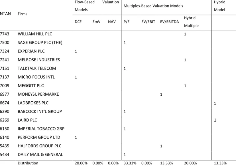
4.4.1 Predominant Models Employed ... 42
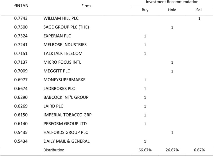
4.4.2 Investment Recommendations ... 44
4.4.3 Forecast Horizons ... 46
4
4.5.1 ROA ... 48
4.5.2 Volatility ... 49
4.5.3 Market Size ... 50
4.6 Final Considerations on the Small Sample Analysis ... 52
5. Conclusion ... 53
6. References ... 55
5
1. Introduction
1.2 Research Context, Motivation
As we gradually become involved by the mists of a new economical paradigm, one less physical and which substance becomes increasingly hard to comprehend and quantify, the elements of the economy accompanied by the instruments that make it move are becoming more intangible in essence themselves. Industries are becoming increasingly knowledge-based and technology intensive, making growing efforts in research and development on behalf of growing innovation needs. The value added by knowledge and innovation is arguably hard to measure but it does make a difference - it is intangible. Today intangible assets have grown to prominence and have earned the right to the spotlight.
This shift to a new economy places on intangible assets an indispensable instrument to preserve firms’ competitive positions and their value creation process.
As defined by the International Accounting Standards (IAS), an asset is a resource that is controlled by a firm as a result of past events from which it expects to benefit economically in the future. The asset category may be differentiated further in line with its tangible or intangible nature as stated by Constantin et al. (1994), be included accordingly in the balance sheet or not, and be created by internal or external sources (Srivastva et al.,1998).
1.2.1 Defining Intangible Assets
Stolowy and Cazan (2001) describe an intangible asset as an identifiable, non-monetary asset, yet lacking physical substance. As suggested by Lev (2004) and Wyatt (2005) patents, trademarks, brands, licenses, technology, employee training, know-how, skilled workforces, customer loyalty, goodwill are all examples of what can be defined as an intangible asset. For their growing importance, intangible assets must be handled and measured appropriately (Vance, 2001) so to avoid creating unbiased and unfair results of firms’ performances (Cañibano et al. 1999).
Due to their nature being difficult to define, the wealth created by intangible assets may not be fully captured by the current accounting standards based on limited recognition criteria. On the other hand, this valuation difficulty may also lead to value overstatement
6 and uncovered investments in the balance sheet. Indeed, financial statements are regarded as unable to fully translate the fair reality of firms’ financial positions whilst offering reliable but perhaps not relevant estimations (Cañibano et al., 2000).
1.3 General Framework
This paper encompasses a study of how equity valuation models perform in measuring the value of firms with high and low proportions of intangibles. It is an attempt to assess whether the differences between the two sets of firms significantly impact the performance of valuation techniques. However, the primary intent of the study is not to offer an outlook of the differences between high and low intangible-intensive industries but rather understand performance variations in valuing firms (and valuation procedures) which intangibles account for a high stake of their total assets and firms in which intangibles account for a rather (conversely) small part of total assets. Ultimately, the goal is to understand how valuation techniques perform in valuing firms in which intangibles assets have great or reduced importance.
With resort to an analysis of a large sample it will be possible to identify the idiosyncrasies of each set of firms whilst also being able to understand which valuation technique is the most appropriate in producing higher quality estimates, in other words, that which returns the lowest valuation error. A subsequent small sample analysis will address the varying approaches of analysts to these contra posing sets of firms.
To this end, a comprehensive review of literature relevant to the matter of equity valuation using accounting numbers will be presented in the next section followed by the results of the large sample analysis. The analysis of the small sample will be covered subsequently which will consist in a review of analysts’ reports followed by an analysis of different patterns and trends underlying the dichotomy high vs low proportion of intangible such as valuation procedures employed, forecast horizons considered and investment recommendations. In addition, a supplemental analysis of some firm specific features such as return on assets, market size and volatility will also be covered. Lastly, the major findings and results will be summarised and the study’s concluding comments will be laid out as to make way for further research.
7
2. Literature review
2.2 Introduction and Debate of the Usefulness of Accounting
Information
As to introduce the reader to more complex financial concepts and the debate of equity valuation and its accounting-based measuring procedures, this section is aimed at explaining what equity valuation is and the importance of accounting information as well as presenting perspectives on equity valuation and its techniques. The contribution of previous academic research to this paper is immeasurable and thus I will resort to an extensive collection of relevant literature to elucidate the reader.
As defined by Lee (1999), equity valuation is a procedure by which the present value of the stream of expected payoffs to shareholders is forecasted. Equity valuation is, therefore, a task of estimating future cash-flows to shareholders and ultimately pricing a firm’s stock as a means to indicate its value. Valuation is instrumental for most levels of business decision.
By 1968, accounting information was still generally considered no to have a substantive meaning thus being seen as of limited use. Accounting practices were bound by how much they were consistent with models of theoretical nature. Ball and Brown (1968) brought change to the accounting practices canons by showing in their work that the studied firms’ yearly income numbers contained at least half of all the available yearly information. In 1989, however, Lev remarks that policy oriented research alike was exceptionally scarce up until then.
Notwithstanding, it was only during the 90s that accounting information had been given major study focus for shareholder value estimation purposes (Lee, 1999).
This has rightfully given recognition to accounting information for the essential role it plays in valuing a business and interpreting a firm’s financial and operational health. Additionally, it acknowledges its paramount importance to forecasting.
Furthermore, recall Lee (1999) who suggested that accounting information plays a facilitating part in the process of valuation but cannot be used as direct measure for firm value. As mentioned before, he elaborates further by stating that equity valuation is
8 itself an estimate of the present value of expected payoffs to shareholders. And because estimates are in essence subjective and inexact, valuation models are compared in terms of inaccuracy rather than precision or perfection.
Many equity valuation models share the same explanatory variable – expected earnings. The variable provides a suitable measure of value (Burgstahler and Dichev, 1997). Beaver (1968) has also debated over earnings. His work shows that earnings reports had information that led to change in investors’ expectations with regards to future returns. By now the reader should have realised the usefulness of accounting information for the purpose of valuing a firm. It is fundamental to assessing a firm’s present realisation just as to foreseeing its future and enabling comparison of figures through and across time and competitors (Ball and Brown, 1968).
2.2.1 Perspectives of Business Valuation
Valuation methods may be seen from two viewpoints. These are the equity (1) and entity (2) perspectives. The equity perspective provides a direct estimation of the value of a firm’s equity whilst the latter estimates the value of the firm’s assets which, in turn, comprise shareholders’ and creditors’ claims.
The equity standpoint estimates the present value of the stream of future dividends. In other words there is no value beyond that of the proprietors – the assets of the owners.
Equity = Assets – Liabilities (1)
Whereas the equity perspective is preferred by most investors and analysts for delivering a more comparable form of valuation, the entity perspective estimates the present value of the Free Cash Flows since they are included in the payoff to shareholders alongside dividends. Furthermore, as it ignores the sources of capital, it avoids the impact of financing decisions and it is not impacted by accounting differences thus making it a preferable option if the previously mentioned effects occur.
9 Under the equity perspective the cost of capital is the cost of equity capital whilst under the entity perspective the cost of capital is represented by the WACC1.
Regardless of the approach taken, the value estimated by an equity based or entity-based valuation models is, theoretically, the same (Palepu et al, 1999).
It is important to refer that the Financial Accounting Standards Board (2008) is the body responsible for the normalisation of the equations presented.
2.3 Accounting-based valuation models
The accounting-based valuation models differentiate between stock-based and flow-based valuation models. The former will hereon forth be referred to as multiples-flow-based valuation model.
2.3.1 Multiples-based Valuation Models
The stock-based, multiples-based models are arguably of easier understanding (Liu et al., 2002) as a result of their intrinsic straightforwardness and simplicity and are a much appreciated method for equity valuation (Carter and Van Auken, 1990). Contrarily to flow-based models they do not make use of multi-period forecasts of a set of parameters. In fact, multiples-based models rely on information from firms which are considered comparable. To this end, comparable firms must similarly reflect the target firm with regards to future cash-flows and exposure to risk.
Ultimately, resorting to comparable firms and benchmark multiples is an exercise of trust in the market. Indeed, there is a reflection of the market in these multiples so the value us considered relative and intrinsic (Palepu et al., 2000).
Demirakos et al., 2004 have shown in their work that multiples-based techniques are the most common used for valuation purposes. This method can be used to value privately held firms which Alford (1992) proved to be useful to value IPOs. Bhojraj and Lee (2002) have also seen that the multiples-based valuation methods are very suitable for the work of investment bankers and not only useful for IPOs but also for M&A activities such as LBOs, SEOs among others.
1 Weighted average cost of capital. It is a cost of capital calculation whereby each category of capital is
10 The estimation of a firm’s value is generated by multiplying a value driver by a multiple acquired from a ratio or an average of the ratios of comparable firms’ stock prices to the value driver (Liu et al., 2002) (3).
𝑉𝑎𝑙𝑢𝑒 𝑜𝑓 𝐹𝑖𝑟𝑚 𝑖 = 𝑉𝑎𝑙𝑢𝑒 𝐷𝑟𝑖𝑣𝑒𝑟𝑖 × 𝐵𝑒𝑛𝑐ℎ𝑚𝑎𝑟𝑘 𝑀𝑢𝑙𝑡𝑖𝑝𝑙𝑒 (3) Although this method may include an intercept, Liu et al. (2002) suggest that its addition may bring added complexity and resulting improvements in performance can only be significantly noticed in poor-performing multiples. The concluding remark is that the complexities would overdo the benefits of including an intercept.
Selecting a value driver is the first step of the multiples-based valuation. This is based on the premise that the value driver is proportional to value. Whether the valuation is performed in accordance to entity or equity perspective is irrelevant as the method suits any of the perspectives. For instance, one could make use of Net Income as an equity value driver or NOPAT as an entity value driver. The following step is the selection of comparable firms which, as previously mentioned, must be similar to the target firm in terms of future cash-flows and risk profile. Lastly, the benchmark multiple is calculated and subsequently applied with resort to equation (3) in order to finally estimated the firm’s value.
2.3.1.1 Selecting the Value Driver
Since value drivers are essential inputs for multiples-based valuations, it is only paramount that these be highly correlated with the firm’s value thus translating the firm’s performance as closely as possible.
The value of the firm is computed recurring to an equation (4) that reflects the product of the value driver, its impact and the benchmark multiple. Several multiples may be used.
𝑉𝑎𝑙𝑢𝑒 𝑜𝑓 𝐹𝑖𝑟𝑚 𝑖 = 𝑊𝑒𝑖𝑔ℎ𝑡1× 𝑉𝐷1,𝑖× 𝐵𝑀1+ 𝑊𝑒𝑖𝑔ℎ𝑡2 × 𝑉𝐷2,𝑖× 𝐵𝑀2 (4) Where VDstands for the value driver which in case there are several are assigned
Weights1,2 and BM is the benchmark multiple of each value driver.
Liu et el. (2002) find that earnings estimated perform significantly better than their reported counterparts. Moreover, P/E multiples were shown to be more suitable to
11 value most firms for its proven superior precision relative to value estimates of cash-flow multiples (Liu et al., 2007). However, as pointed out in their work, earnings can be a target of manipulation and opportunism from management leading to transitory items not related to the firm’s inherent features influencing the value estimate rather negatively (Liu et al., 2007).
2.3.1.2 Selecting comparable firms
Comparables are of particular interest as they can be of use in performing fundamental analysis and forecasting sales growth ratios and profit margins (Bhojraj and Lee, 2002). The choice for a comparable should contemplate variables that explain cross-sectional differences in multiples thus ensuring the similarity between the multiples of the comparables and the multiple of the target firm (Alford, 1992). To this end, one can either fetch an individual comparable firm or, alternatively, make use of a set of comparable firms. Finding one single comparable that is similar to the target firm is easy but its differences will reflect rather greatly, irrespective of how small they are when compared to a multiple resultant of a set of comparables. Conversely, firm-specific differences will be annulled if the benchmark multiple is computed with resort to the set of comparables.
Nevertheless, the conclusion drawn by Liu et al. (2002) was that the performance of multiples-based models was rather inferior when all the firms in the cross-section were selected as comparables.
As Palepu et al. (2002) stated, even when rigorously defined, there are industries that lay down serious barriers to finding appropriate multiples. Differences in strategy, profitability and goals, for example, pose comparability problems (Liu et al., 2002). Alford (1999) has shown that choosing comparable firms from the same industry improved accuracy with the increase in the number of SIC digits.
Despite resulting mostly in appropriate valuations, the selection of comparables based on their industry may lead to failure if the industry is not properly defined (Alford, 1992 and Liu et al., 2002). In effect, future enterprise value-to-sales and price-to-book ratios have been shown to greatly increase efficacy in comparison to industry and size based
12 criteria (Bhojraj and Lee, 2002), which leaves room to reconsider the fittingness of industry based comparables in generating appropriate multiples.
2.3.1.3 Calculating the Benchmark Multiple
In order to obtain an appropriate benchmark multiple, any of the following estimators can be used:
𝐴𝑟𝑖𝑡ℎ𝑚𝑒𝑡𝑖𝑐 𝐴𝑣𝑒𝑟𝑎𝑔𝑒 (𝑀𝑒𝑎𝑛) =𝑛1∑ 𝑃𝑗 𝑉𝐷𝑗 𝑛
𝑗=1 (5)
Median = value halfway between observed maximum and minimum (6)
𝑊𝑒𝑖𝑔ℎ𝑡𝑒𝑑 𝐴𝑣𝑒𝑟𝑎𝑔𝑒 = ∑ ( 𝑉𝐷𝑗 ∑𝑛𝑖=1𝑉𝐷𝑖) × 𝑃𝑗 𝑉𝐷𝑗 𝑛 𝑗=1 = ∑𝑛𝑗=1𝑃𝑗 ∑𝑛𝑗=1𝑉𝐷𝑗 (7) 𝐻𝑎𝑟𝑚𝑜𝑛𝑖𝑐 𝑀𝑒𝑎𝑛 = (𝑛1∑ 𝑉𝐷𝑗 𝑃𝑗 𝑛 𝑗=1 ) −1 (8)
The Value driver being represented by VDi and the Price of the jth comparable firm by Pi.
The arithmetic average, or mean, is the most widely adopted method and is frequently employed by analysts (Liu et al., 2002). However, its use often results in overvaluation due to the presence of outliers that significantly distort information thus being rather upward biased. All in all, mean estimators will frequently return larger values than harmonic mean (Baker and Ruback, 1999). In fact, Liu et al. (2002) found that the use of harmonic mean improves the performance of multiples-based valuation due to the reduced influence of small denominators. Consistently, Baker and Ruback (1999) had already shown that the performance of the harmonic mean (8) is greater than that of the remaining estimators.
2.3.2 Flow-based Valuation Models
In 2000, Francis et al. verified an equality between the market value of a share and the discounted value of the expected future payoffs derived from the share. This assumption sets the ground for flow-based models.
Despite being hard to obtain identical results in practice because of changing input forecasts, growth rates and/or discount rates, theoretically the returned value should be correspondent (Francis et al., 2000 and Corteau et al. 2006).
13 The discounted dividend model and the discounted cash flow model, on which I will elaborate next, are the cornerstone for accounting-based valuation as the other methods have been derived from these and adapted to comprise accounting information and thus capture its effects.
2.3.2.1 Discounted Dividend Model (DIV)
The formulation of the discounted dividend model is credited to Williams (1999) and establishes the following equality
𝐸𝑞𝑢𝑖𝑡𝑦 𝑉𝑎𝑙𝑢𝑒𝐹𝐷𝐼𝑉 = ∑ 𝐸𝑥𝑝𝑒𝑐𝑡𝑒𝑑 𝐷𝑖𝑣𝑖𝑑𝑒𝑛𝑑𝑡 (1+𝑟𝑒)𝑡 𝑇
𝑡=1 (9)
Where, re denotes cost of equity capital, F the valuation date and T the expected end
date of the firm.
In other terms, its premise is that a firm’s equity is equal to the sum of the discounted expected dividends due to be received by shareholders over the firm’s lifespan. Dividends correspond to the cash flows distributed to the shareholders (Penman, 2007). Therefore, it is the present value of the expected future cash dividends (Ross et al., 2008). The terminal value is equal to the liquidating dividend (Francis et al., 2000). The DIV is viewed as the easiest model to employ due to forecasting being considered simple and straightforward to perform, if stable dividend policies are assumed (Brealey et al., 2005 and Penman, 2008)
It is important to note though, that depending on certain conditions the aforementioned formula might have to suffer alterations. The formula may be adapted to accommodate, for instance, a setting where a firm pays a constant steady dividend, or alternatively a constant growing dividend, and has no expectation of life termination2.
14 A noticeable opposition to this model can be found in Modigliani and Miller’s (1961) work on dividend irrelevance. However, literature has further verified the impact of dividend policy in stock price. (Walter, 1956, Black and Scholes, 1974 and Fisher 1961). As mentioned previously, valuation models stem from DIV and are, indeed, a reference for most of the valuation procedures (Barker, 2001).
2.3.2.2 Discounted Cash-flow Model (DCF)
The discounted cash-flow model involves estimating the cash flows of a firm by discounting them at a rate that carries an identical risk level (Lie and Lie, 2002). The DCF estimator is as follows:
𝐸𝑛𝑡𝑒𝑟𝑝𝑟𝑖𝑠𝑒 𝑉𝑎𝑙𝑢𝑒𝐹𝐷𝐶𝐹 = ∑ 𝐹𝐶𝐹𝑡 (1+𝑟𝑊𝐴𝐶𝐶)𝑡 𝑇
𝑡=1 (12)
The FCF (13) is considered to more accurately reflect value added over a short horizon (Francis et al., 2000) and is discounted at the weighted average cost of capital (14). 𝐹𝐶𝐹𝑡 = 𝑁𝑂𝑃𝐴𝑇 + 𝐶ℎ𝑎𝑛𝑔𝑒 𝑖𝑛 𝑁𝑒𝑡 𝑂𝑝𝑒𝑟𝑎𝑡𝑖𝑛𝑔 𝐴𝑠𝑠𝑒𝑡𝑠 − 𝐶𝑎𝑠ℎ 𝐼𝑛𝑣𝑒𝑠𝑡𝑚𝑒𝑛𝑡𝑠 (13) 𝑟𝑊𝐴𝐶𝐶 = 𝜔𝑑 × (1 − 𝜏) × 𝑟𝑑+ 𝜔𝑃𝑆× 𝑟𝑃𝑆+ 𝜔𝑒× 𝑟𝑒 (14)
Where 𝜏 stands for corporate tax rate, 𝜔𝑑,𝑃𝑆,𝑒 refers to proportion of debt, preferred stock and equity respectively, and 𝑟𝑑,𝑃𝑆,𝑒 to cost of debt, preferred stock and equity respectively.
2.3.2.3 Residual Income Model (RIVM)
Residual income takes an instrumental part in equity valuation being used as a performance measure (O’Hanlon, 2002). It corresponds to the earnings that are net of capital costs. The model reflects the premium over book value given by the market due to increase or decrease in expected book values (Ohlson, 2005)3.
From the equity perspective, residual income is calculated as follows: 𝑅𝑒𝑠𝑖𝑑𝑢𝑎𝑙 𝐼𝑛𝑐𝑜𝑚𝑒𝑡𝑒 = 𝑁𝑒𝑡 𝐼𝑛𝑐𝑜𝑚𝑒
𝑡− 𝑟𝑒× 𝐵𝑉𝐸𝑡−1 (15.1)
Where BE stands for book value of equity.
15 From the entity perspective, residual income is calculated as follows:
𝑅𝑒𝑠𝑖𝑑𝑢𝑎𝑙 𝐼𝑛𝑐𝑜𝑚𝑒𝑡𝑒+𝑑 = 𝑁𝑂𝑃𝐴𝑇
𝑡− 𝑟𝑊𝐴𝐶𝐶× 𝑁𝑂𝐴𝑡−1 (15.2)
Where NOA stands for net operating assets.
Furthermore, the RIVM must verify the clean surplus relationship (CSR) which is represented by the equality between the change in shareholders’ equity and Net income less net dividends (Lundholm and O’Keefe, 2001).
The formulae below translate that relationship, seen from the equity and entity perspectives, respectively:
𝐵𝑉𝐸𝑡− 𝐵𝑉𝐸𝑡−1= 𝑁𝑒𝑡 𝐼𝑛𝑐𝑜𝑚𝑒𝑡− 𝐷𝑖𝑣𝑖𝑑𝑒𝑛𝑑𝑡 (16.1)
𝑁𝑂𝐴𝑡− 𝑁𝑂𝐴𝑡−1 = 𝑁𝑂𝑃𝐴𝑇𝑡− 𝐹𝐶𝐹𝑡 (16.2)
Nevertheless, despite being in accordance to the balance sheet principles this relationship may not verify as the way GAAP sees earnings is incompatible with clean surplus accounting (Ohlson, 2005). As Ohlson states, dirty surplus items must be assumed to be insignificant (marginally equal or close to zero).
The RIVM estimator is built by adjusting the DIV estimator in order to accommodate a rearranged definition of dividend that will encompass residual income. Residual income will now be embedded in the following new estimators both from the equity perspective (17.1) and entity perspective (17.2):
𝐸𝑞𝑢𝑖𝑡𝑦 𝑉𝑎𝑙𝑢𝑒𝑡= 𝐵𝑉𝐸𝑡+ ∑ 𝐸𝑡[𝑅𝑒𝑠𝑖𝑑𝑢𝑎𝑙 𝐼𝑛𝑐𝑜𝑚𝑒𝑡+𝜏𝑒 ] (1+𝑟𝑒)𝜏 ∞ 𝜏=1 (17.1) 𝐸𝑛𝑡𝑒𝑟𝑝𝑟𝑖𝑠𝑒 𝑉𝑎𝑙𝑢𝑒𝑡= 𝑁𝑂𝐴𝑡+ ∑ 𝐸𝑡[𝑅𝑒𝑠𝑖𝑑𝑢𝑎𝑙 𝐼𝑛𝑐𝑜𝑚𝑒𝑡+𝜏𝑒+𝑑] (1+𝑟𝑊𝐴𝐶𝐶)𝜏 ∞ 𝜏=1 (17.2)
As Lee and Swathimanathan (1999) note, the equity perspective (17.1) breaks firm value into two components, these being capital invested (BVE) and the present value of the future value create, which is the sum of future residual income.
The RIVM has the advantage of not being affected by dividend or accounting policies. As Francis et al. (2000) have seen, dividends have no influence on the value of equity nor accounting policies impact the clean surplus relationship. Additionally, RIVM has been
16 found to estimate equity value more accurately than DIV or DCF while explaining 71% of changes in prices (Francis et al., 2002). Arguably, distortions in book values have a smaller impact than discount and growth rates estimation errors leading to differences in valuation results between RIVM in relation to DIV and DCF. Francis et al. claim, in addition, that residual income is easier to predict and that might be one of the reasons for RIVM’s greater precision.
2.3.2.3.1 Implementation issues
The RIVM may pose some implementation complications though. Cost of equity, earnings forecasts, forecast horizons, dividend pay-out ratios, terminal values are all sources of possible barriers to properly implementing RIVM (Lee and Swaminathan, 1999).
To begin with, cost of equity is calculated according to the CAPM4 (Lee and Swaminathan, 1999) as follows:
𝑟𝑒= 𝑟𝑓+ 𝛽 × (𝑟𝑚− 𝑟𝑓) (18)
Then, to forecast earnings one must resort to return on equity (ROE) which can be derived from the CSR5. Indeed, I/B/E/S consensus forecasts are highly correlated with current stock prices (Frankel and Lee, 1998). The RIVM proved to be able to explain more than 70% of cross-sectional price variation.
Long-term RI can be estimated in one of two possible ways. These are using analysts’ long term growth forecasts (Frankel and Lee, 1998) and assume that ROE fades gradually in time, converging into the industry’s average (Lee and Swaminathan, 1999).
The terminal value (TV) provides an estimate of the future RI (18)6. 𝑇𝑉 = ∑ 𝐸𝑡[𝑅𝑒𝑠𝑖𝑑𝑢𝑎𝑙 𝐼𝑛𝑐𝑜𝑚𝑒𝑡+𝜏𝑒 ] (1+𝑟𝑒)𝜏 ∞ 𝜏=𝑇+1 =𝐸𝑡[𝑅𝑒𝑠𝑖𝑑𝑢𝑎𝑙 𝐼𝑛𝑐𝑜𝑚𝑒𝑡+𝑇 𝑒 ]×(1+𝑔 𝑟) (1+𝑟𝑒)𝑇×(𝑟𝑒−𝑔𝑟) (19) 4 R
f stands for the risk free rate, β denotes the firm’s beta and rm is the market return. The risk free rate
can be based on a short-term treasury bill or a long-term treasury bond (Lee and Swaminathan, 1999). Whereas, the market premium can be determined by (rm-rf), the market return can be indirectly
determined by randomly estimating market premium, historically around 5% (Lee and Swaminathan, 1999).
5 Note that book values can be obtain from the clean surplus relationship 6 g
17 Seen from the equity perspective, RIVM suffers some adaptations in relation to previously presented equations.
𝐸𝑞𝑢𝑖𝑡𝑦 𝑉𝑎𝑙𝑢𝑒𝑡 = 𝐵𝑉𝐸𝑡+ ∑ 𝐸𝑡[𝑅𝑒𝑠𝑖𝑑𝑢𝑎𝑙 𝐼𝑛𝑐𝑜𝑚𝑒𝑡+𝜏𝑒 ]
(1+𝑟𝑒)𝜏
𝑇
𝜏=1 + 𝑇𝑉 (20)
It is important to recall that in presence of the clean surplus relationship, RIVM, DIV and DCF must, theoretically, provide an absolute match in terms of value.
2.3.2.4 Abnormal Earnings Growth Model (AEGM)
The abnormal earnings growth model (AEGM) was designed by Ohlson and Juettner-Nauroth and is an expanded version of the RIVM that embeds forthcoming-period expected EPS and prospective growth in earnings. Ohlson claims that AEGM model’s estimator (21) include concepts which are more familiar to analysts.
𝐸𝑞𝑢𝑖𝑡𝑦 𝑉𝑎𝑙𝑢𝑒𝑡 =𝐸𝑡[𝑁𝐼𝑡+1] 𝑟𝑒 + ∑ 𝐸𝑡[𝑧𝑡+𝜏] (1+𝑟𝑒)𝜏 𝑇 𝜏=1 + ∑ 𝐸(1+𝑟𝑡[𝑧𝑡+𝜏] 𝑒)𝜏 ∞ 𝜏=𝑇+1 , and (21) 𝑧𝑡 =𝑟1 𝑒× (∆𝑁𝐼𝑡+1− 𝑟𝑒× (𝑁𝐼𝑡− 𝐷𝐼𝑉𝑡)) (22)
Where NI represents net income (earnings) and ∆𝑁𝐼𝑡+1 its variation.
Notice that the comparable RIVM estimator (23) is remarkably analogous to the AEGM (21) as both rely on a certain forecast horizon and a terminal value.
𝐸𝑞𝑢𝑖𝑡𝑦 𝑉𝑎𝑙𝑢𝑒𝑡 = 𝐵𝑉𝐸𝑡+ ∑ 𝐸𝑡[𝑅𝐼𝑡+𝜏𝑒 ] (1+𝑟𝑒)𝜏 𝑇 𝜏=1 + ∑ 𝐸𝑡[𝑅𝐼𝑡+𝜏 𝑒 ] (1+𝑟𝑒)𝜏 ∞ 𝜏=𝑇+1 (23)
The differences fall into the AEGM being based on realised next-period earnings which account for a very significant part of the resulting valuation and the RIVM being based on current book value. The terminal value impacts AEGM to a lesser extent as in implication of the next period earnings comprising a rather significant part of the resulting valuation. Ohlson and Juettner-Nauroth, 2005 add that since the AEGM is not impacted by dividend policy it relies less on the CSR and more on earnings. Most importantly, the authors emphasize that next period realised earnings are a closer proxy to market value than book value.
18
2.3.3 Final Considerations on the Accounting-based Valuation
Models
There are some important considerations to highlight. Firstly, recall Amir and Lev (1996) who importantly pointed out that information of non-financial nature can be an important value driver. In addition, consider that the extent of information available influences the performance of the valuations methods. This means that, in general, the application of these techniques works better in more matured firms within rather conventional industries of which more information is known. Amir and Lev (1996) rightly outlined that some industries imply different accounting treatments and this means there are several valuation models of less conventional nature which may be able to perform more price estimates.
Particularly, information deficit has interesting implications in bankruptcy situations and IPOs. Gilson et al. (2000) had seen that in situations of bankruptcy, because information was missing, both multiples-based and cash-flow based techniques delivered poor valuation performances despite being, in fact, unbiased. Similarly, Kim and Ritter (1999), and Gilson et al. (2000) had also seen that DCF also fails to accurately valuate firms due to difficulties in estimating cash-flows.
As mentioned before, other procedures can be employed to estimate value in case of industries and firms with peculiar features. For instance, R&D spending was proven to be an appropriate value driver for Biotech IPOs (Guo et al., 2005).
19
2.4 Conclusion on the Literature Review
The purpose of this review of relevant literature was to introduce the concepts of intangible assets and highlight the importance of accounting information in firm valuation (Ball and Brown, 1968). Moreover, it presented the most prominent flow-based and multiples-flow-based valuation models, while explaining that although these models should, in theory, provide identical results, they deliver varying performances (Francis et al., 2000 and Courteau et al., 2006). Ultimately we have seen that, even though the RIVM has been shown to be more precise (Francis et al., 2000), multiples-based methods are the most widely employed (Demirakos et al., 2004). Nevertheless, valuation techniques depend on the nature and availability of the information, returning different results according to industries and firm specificities.
20
3. Large sample analysis
3.2 Introduction
3.2.1 Contextualising the Large Sample Analysis and Developing of
Hypotheses
As seen previously in this paper, accounting information does not reflect entirely the true value of a firm. Firms that are R&D intensive, that engage in strong advertising or with high level of investments fail to see these efforts reflect in their balance sheets thus not portraying a fair reality of their final position. Notwithstanding, it has been seen that the valuation effect of intangible assets in the market value of firms is more important than that of the tangible assets (Hall, 2001). It is from this premise that it becomes interesting to understand how different proportions of intangibles behave depending on the valuation methods.
Valuation techniques should, in theory, provide identical results. However, it is because some models can, in fact, deliver a superior performance due to differing assumptions and input variables that it is relevant to ask the following question:
Research question: Do P/E multiple and RIVM perform worse in valuing firms with a high
ratio of Intangible Assets to Total Assets (PINTAN)?
This chapter intends to provide a comprehensive insight on the differences in valuations delivered by different valuation methods. The goal is to understand whether firms that present higher proportions of intangible assets relatively to the totality of their assets are significantly more difficult to valuate. Whereas the proportion of intangibles better reflects the reality of the firm as it is a relative measure, studying intangibles in absolute would not allow for an appropriate sample selection and thus drawing proper conclusions from a representative sample. To this end, proportion of intangibles (PINTAN) has been used. Furthermore, the hypothesis of one valuation method providing a superior, more precise valuation than other is also considered and analysis is conducted for this purpose. Finally, the paper will also evaluate if performance is different across years, for which it is believed changes in economic conjuncture are a cause, and across industries due to industry-specific features.
21 As a result of the scope of the large sample and, in great part, of the scope of this paper, the hypotheses developed follow below:
Hypothesis 1: High proportion of intangibles implies inferior performance of valuation
models than low PINTAN.
Hypothesis 2: RIVM performs better than P/E. Hypothesis 3: Performance is unequal across years. Hypothesis 4: Performance is unequal across industries.
3.3 Research design
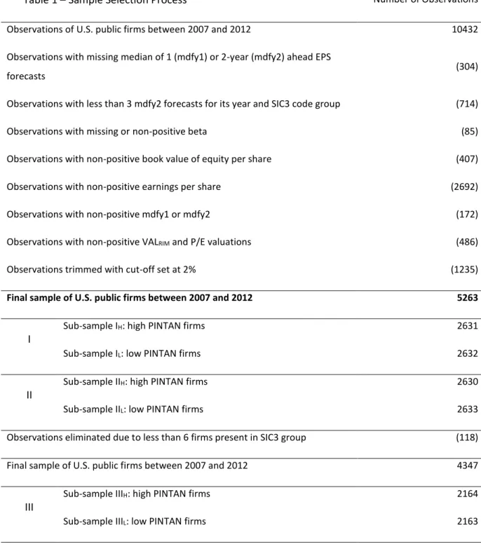
3.3.1 Data and Sample Selection
The raw dataset was retrieved from Compustat, I/B/E/S7 and CRSP8. Note that Compustat data was adjusted to be consistent to I/B/E/S already adjusted stock split/dividend9.
The sample comprised an initial number of 10432 observations of publicly traded US firms which stocks have been traded from December 2007 to December 201210. However, as to construct an appropriate dataset for analysis, some exclusion criteria have been put in practice. Observations lacking fundamental information that is required for later calculations as, for instance, in valuation models or other supporting computations must be disregarded in order to enable an analysis that is representative and with significance. Hence, to begin with, observations with non-available information regarding the median of 1 and/or 2 year ahead earnings per share (EPS) forecasts were eliminated. Subsequently, observations with non-available and/or non-positive beta were deleted for further cost of capital calculation purposes. Also, to comply with the requisites of the valuation models employed, further deletion of observations with
7 I/B/E/S provides analysts forecasts and market prices. 8 CRSP provides betas.
9 A full list of variables (Table 2) and the adjustment procedures (24) (25) are included in appendix. 10 Refer to Fiscal Years 2006-2011.
22 positive EPS, BPS and/or mdfy1 and/or mdfy2 was conducted followed by the final elimination of those which revealed non-positive P/E ratios.
The resulting dataset was then trimmed in 2% - in both sides – to account for the distorting effect of extreme observations (outliers) thus ensuring greater statistical representativeness of the sample. The choice of trimming the sample in 2% falls into the fact that a first 1% cut-off attempt did not effectively eliminate all the extreme observations.
Consistent with the dichotomy underlying this paper, the resulting sample has ultimately been divided into High Proportion of Intangibles (IH) and Low Proportion of Intangibles (IL)11. The median of the proportion of intangibles (PINTAN) was set as the reference and threshold for high and low meaning that a high proportion of tangibles is above that median and low below the median.
Finally, the ultimate samples were replicated and altered twice. First, high and low are determined relatively to the respective year’s median12 PINTAN (in contrast to the whole sample’s median) and second, high and low are determined relatively to each SIC3 group PINTAN median13. This has been done so that it can be confirmed whether the classification given for high and low PINTAN is impacting the analysis.
11 Quartile division was initially considered but later abandoned. Division in half allowed for a larger
number of observations and thus greater statistical power.
12 Refer to Sample II
H and IIL in appendix – Table A 13 Refer to Sample III
23 Below is a breakdown of the stages for selecting the final sample.
Table 1 – Sample Selection Process Number of Observations Observations of U.S. public firms between 2007 and 2012 10432
Observations with missing median of 1 (mdfy1) or 2-year (mdfy2) ahead EPS
forecasts (304)
Observations with less than 3 mdfy2 forecasts for its year and SIC3 code group (714)
Observations with missing or non-positive beta (85)
Observations with non-positive book value of equity per share (407)
Observations with non-positive earnings per share (2692)
Observations with non-positive mdfy1 or mdfy2 (172)
Observations with non-positive VALRIM and P/E valuations (486)
Observations trimmed with cut-off set at 2% (1235)
Final sample of U.S. public firms between 2007 and 2012 5263
I
Sub-sample IH: high PINTAN firms 2631
Sub-sample IL: low PINTAN firms 2632
II
Sub-sample IIH: high PINTAN firms 2630
Sub-sample IIL: low PINTAN firms 2633
Observations eliminated due to less than 6 firms present in SIC3 group (118)
Final sample of U.S. public firms between 2007 and 2012 4347
III
Sub-sample IIIH: high PINTAN firms 2164
24
3.3.2 Research Methods
3.3.2.1 Residual Income Valuation Model (RIVM)
Due to its demonstrated better performance in comparison to DIV (Francis et al., 2000), the RIVM14 was the selected flow-based valuation model.
𝑉𝐴𝐿𝑅𝐼𝑉𝑀 = 𝐵𝑃𝑆 + 𝑅𝐼1 1+𝐾𝐸+
𝑅𝐼2 (𝐾𝐸−𝐺)⁄
1+𝐾𝐸 (26)
RI1 (34) and RI2 (35) were calculated using median forecasts retrieved from I/B/E/S to ensure that extreme values do not exert unwanted influence. Note that Frankel and Lee (1998) had seen in their work that residual income is highly correlated with stock prices.
KE, in turn, stands for the cost of capital. This is calculated recurring to equation 20 covered in the previous chapter, assuming a risk free rate based on a 90-day annualised T-Bills yearly average and a 5% market premium (Lee and Swaminathan, 1999). The CRSP is the source of the beta.
The dividend pay-out ratio is calculated as follows: 𝐷𝑃𝐴𝑌𝑂𝑈𝑇 = 𝐷𝑉𝐶
0.05×𝐴𝑇 (27)
In accordance with the work of Lee and Swaminathan (1999), dividend pay-out ratio (27) equals one if the last reported ratio is higher than one whilst it is set to equal the firm’s average return of assets if EPS are below zero.
3.3.2.2 Price to Earning (P/E) Multiple
The multiples-based valuation model employed is based on the price to earnings ratio. As a value driver, the 2 year ahead forecasted median was selected as it is able to mitigate the impact of extreme observations. In addition, it is considered to have greater explanatory power (Liu et al., 2002).
The benchmark multiple was calculated with resort to a harmonic mean (8) which has been shown by Liu et al. (2002) to improve performance.
𝑉𝐻𝑀𝐸𝐴𝑁𝑃𝐸 = 𝑀𝐷𝐹𝑌2 × 𝐻𝑀𝐸𝐴𝑁𝑃𝐸 (36)
Based on the work of Alford (1992), the comparable firms were firms included in the same SIC3 group code and fiscal year.
25
3.3.2.3 Errors and Measure of Performance
In order to evaluate performance one must look at the errors in valuation.
The signed error is a measure of bias. As such it measures the propensity for overvaluation, in case of negative signed error, and undervaluation, in case of positive signed error.
𝑆𝑖𝑔𝑛𝑒𝑑 𝐸𝑟𝑟𝑜𝑟 =𝑃𝑟𝑖𝑐𝑒−𝑉𝑎𝑙𝑢𝑒 𝐸𝑠𝑡𝑖𝑚𝑎𝑡𝑒𝑃𝑟𝑖𝑐𝑒 (37)
In contrast, the absolute error measures inaccuracy and shows how distant the value estimate is comparatively to the market price.
𝐴𝑏𝑠𝑜𝑙𝑢𝑡𝑒 𝐸𝑟𝑟𝑜𝑟 =|𝑃𝑟𝑖𝑐𝑒−𝑉𝑎𝑙𝑢𝑒 𝐸𝑠𝑡𝑖𝑚𝑎𝑡𝑒|
𝑃𝑟𝑖𝑐𝑒 (38)
3.4 Descriptive Statistics
3.4.1 General Descriptive Statistics
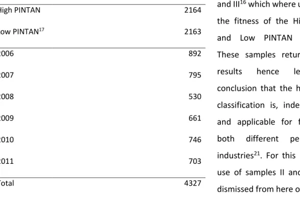
The table below summarises the number of observations in each division and in each year of the general sample (sample I).
Table 3 – Observations per sub-sample and fiscal Year High PINTAN Low PINTAN17 2164 2163 2006 892 2007 795 2008 530 2009 661 2010 746 2011 703 Total 4327
It is relevant to recall samples II15 and III16 which where use to verify the fitness of the High PINTAN and Low PINTAN definitions. These samples return identical results hence leading to conclusion that the high vs. low classification is, indeed, correct and applicable for firm across both different periods and industries21. For this reason, the use of samples II and III will be dismissed from here on.
15 Sample II, refer to table A for descriptive statistics. 16 Sample III, refer to table B for descriptive statistics.
26 Table 4 - Sample I Descriptive Statistics
Panel I: Combined Sample I N Mean Standard
Deviation Median Minimum Q1 Q3 Maximum
Share Price in April (P4) 4327 30.3133 19.1342 26.4600 2.8500 16.0000 39.8200 135.1500 Common Equity per Share (BPS) 4327 13.1856 8.9608 11.1124 0.6975 6.4211 17.8813 56.2731 EPS Excl. Extraordinary Items (EPS) 4327 1.7321 1.3817 1.3900 0.0350 0.7300 2.3300 10.3900
PINTAN 4327 0.2011 0.2033 0.1361 0.00 0.0222 0.3325 0.7722
Median 1-Year-Ahead EPS (MDFY1) 4327 1.8720 1.2533 1.5800 0.0200 0.9100 2.5300 6.9100 Median 2-Year-Ahead EPS (MDFY2) 4327 2.1766 1.3745 1.8500 0.2500 1.1300 2.9000 7.4600
Panel II: Sub-Sample IL N Mean
Standard
Deviation Median Minimum Q1 Q3 Maximum
Share Price in April (P4) 2164 29.6286 18.5642 25.7200 3.9000 16.2100 38.8900 135.1500 Common Equity per Share (BPS) 2164 13.2969 9.1397 11.0827 0.8362 6.2074 18.6015 56.2731
EPS Excl. Extraordinary Items (EPS) 2164 1.7724 1.4318 1.4200 0.0350 0.7700 2.3675 10.3900
PINTAN 2164 0.0376 0.0404 0.0223 0.00 0.00 0.0678 0.1361
Median 1-Year-Ahead EPS (MDFY1) 2164 1.8211 1.2195 1.5300 0.0300 0.8900 2.5000 6.9100 Median 2-Year-Ahead EPS (MDFY2) 2164 2.1243 1.3269 1.8300 0.2500 1.1100 2.8000 7.4600
Panel III: Sub-Sample IH N Mean
Standard
Deviation Median Minimum Q1 Q3 Maximum
Share Price in April (P4) 2163 30.9984 19.6685 27.1500 2.8500 15.7300 40.8900 123.5900 Common Equity per Share (BPS) 2163 13.0741 8.7790 11.1250 0.6975 6.6155 17.1997 55.1717 EPS Excl. Extraordinary Items (EPS) 2163 1.6918 1.3288 1.3600 0.0400 0.7000 2.3200 9.3700 PINTAN 2163 0.3646 0.1659 0.3325 0.1361 0.2242 0.4784 0.7722 Median 1-Year-Ahead EPS (MDFY1) 2163 1.9229 1.2845 1.6200 0.0200 0.9300 2.5900 6.6500 Median 2-Year-Ahead EPS (MDFY2) 2163 2.2289 1.4189 1.8700 0.2700 1.1500 3.0000 7.3100
27 The fragmentation into sub-samples lets isolate certain specificities associated to the high or low intangible proportion nature of the observations.
From the results provided by the above descriptive statistics, it is worth directing attention to the fact that the mean of stock price is highest for high PINTAN observations. One may consequently infer that investors favour high PINTAN firms, valuing it significantly more. Conversely, the low intangible proportion sub-sample indicates the highest EPS. Since EPS is strongly associated to operating income, it was only to be expected that firms with a lower proportion of intangibles return higher results in this case. However, BPS is meaningfully lower for firms with a high proportion of intangibles despite the higher average market prices. The conclusion is that the market maintains expectations for higher return on equity in firms with a higher proportion of intangibles.
Sample I exhibits a mean that is well above the median mainly due to the fact that while minimum values where limited to values higher than zero for several variables, the maximum values are large enough to end up producing a significant impact in the results17.
28
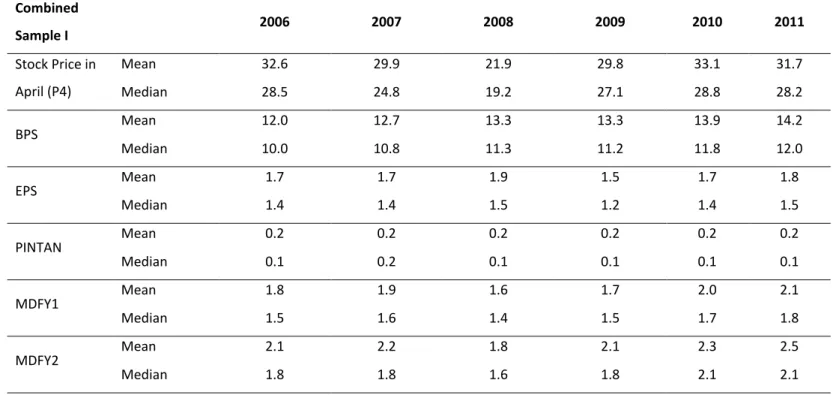
3.4.2 Descriptive Statistics by Fiscal Year
An interesting observation that is worth the exhibition of the table below is that from years 2006 to 2008 there is a visible decline in mean stock price which reflects a negative economic conjuncture followed by a recovery from 2009 until 2011.
Table 5 – Sample I Descriptive Statistics by Fiscal Year.
Combined Sample I 2006 2007 2008 2009 2010 2011 Stock Price in April (P4) Mean 32.6 29.9 21.9 29.8 33.1 31.7 Median 28.5 24.8 19.2 27.1 28.8 28.2 BPS Mean 12.0 12.7 13.3 13.3 13.9 14.2 Median 10.0 10.8 11.3 11.2 11.8 12.0 EPS Mean 1.7 1.7 1.9 1.5 1.7 1.8 Median 1.4 1.4 1.5 1.2 1.4 1.5 PINTAN Mean 0.2 0.2 0.2 0.2 0.2 0.2 Median 0.1 0.2 0.1 0.1 0.1 0.1 MDFY1 Mean 1.8 1.9 1.6 1.7 2.0 2.1 Median 1.5 1.6 1.4 1.5 1.7 1.8 MDFY2 Mean 2.1 2.2 1.8 2.1 2.3 2.5 Median 1.8 1.8 1.6 1.8 2.1 2.1
The abovementioned adverse economic climate can be more easily observed in the time series chart plotted below:
1 1,5 2 2,5 3 3,5 4 4,5 5 15 17 19 21 23 25 27 29 31 33 35 2006 2007 2008 2009 2010 2011
Chart 1 - Mean and Median Evolution 2006-2011
mean, p4 median, p4 mean, EPS median, EPS
29
3.5 Data Analysis
3.5.1 Signed and Absolute Errors
3.5.1.1 Descriptive Statistics
3.5.1.1.1 General Descriptive Statistics
Performance is assessed in terms of accuracy and bias with resort to an analysis of the valuation errors. Recall that bias is positive when signed errors are negative and vice versa implying overestimation and underestimation respectively18.
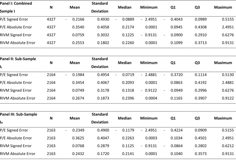
Valuation errors’ descriptive statistics presented in the table below show that RIVM apparently performs better than P/E, having signed and absolute errors closer to zero. Additionally, it is curious to note that P/E is on average overvaluing firms and RIVM undervalues them, although to a lesser absolute degree.
Table 6 - Sample I Descriptive Statistics
Panel I: Combined
Sample I N Mean
Standard
Deviation Median Minimum Q1 Q3 Maximum
P/E Signed Error 4327 - 0.2166 0.4930 - 0.0889 - 2.4951 - 0.4043 0.0989 0.5155 P/E Absolute Error 4327 0.3540 0.4058 0.2174 0.0001 0.0945 0.4308 2.4951 RIVM Signed Error 4327 0.0759 0.3032 0.1225 - 0.9131 - 0.0900 0.2910 0.6276 RIVM Absolute Error 4327 0.2553 0.1802 0.2260 0.0001 0.1099 0.3713 0.9131
Panel II: Sub-Sample IL
N Mean Standard
Deviation Median Minimum Q1 Q3 Maximum
P/E Signed Error 2164 - 0.1984 0.4954 - 0.0719 - 2.4881 - 0.3720 0.1114 0.5130 P/E Absolute Error 2164 0.3454 0.4067 0.2093 0.0001 0.0863 0.4192 2.4881 RIVM Signed Error 2164 0.0749 0.3178 0.1318 - 0.9122 - 0.0949 0.2996 0.6276 RIVM Absolute Error 2164 0.2674 0.1873 0.2396 0.0004 0.1165 0.3907 0.9122
Panel III: Sub-Sample IH
N Mean Standard
Deviation Median Minimum Q1 Q3 Maximum
P/E Signed Error 2163 - 0.2349 0.4900 - 0.1179 - 2.4951 - 0.4224 0.0909 0.5155 P/E Absolute Error 2163 0.3625 0.4047 0.2263 0.0003 0.1034 0.4501 2.4951 RIVM Signed Error 2163 0.0768 0.2879 0.1125 - 0.9131 - 0.0864 0.2802 0.6212 RIVM Absolute Error 2163 0.2432 0.1720 0.2141 0.0001 0.1040 0.3573 0.9131
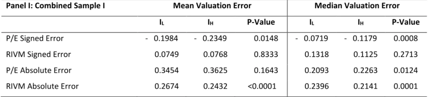
30 Apart from the RIVM’s superior performance regarding average valuation errors, it should be added that it is more reliable as its standard deviation is much lower, consequently leading to a smaller effect of extreme values. This fact is visible by looking at both models’ maximum absolute errors. While the RIVM’s absolute error does not exceed 100%, the multiple based valuation model has a maximum absolute error of nearly 250%.
Regarding the differences between high and low PINTAN, it is noticeable a slight improvement on average absolute errors in P/E valuation of low PINTAN firms and the opposite change in RIVM absolute errors, which performs better on high PINTAN firms. Although there is no significant variation in RIVM bias, it is noteworthy the increase in positive bias by P/E valuations on high PINTAN.
Finally, it is remarkable that for high PINTAN firms the median performance is nearly equal for both models’ absolute errors and that they are contrarily biased but in the same degree. Naturally, the abovementioned skewness of P/E valuation errors shows that there are more extreme values for this model’s valuation estimates.
3.5.1.1.2 Descriptive Statistics by Fiscal Year and SIC3
An additional view on the valuation errors is relevant this time to understand how they differ depending on the years and industries and contest the hypotheses set earlier in this paper.
Hypothesis 3: The level of performance is unequal across years Hypothesis 4: The level of performance is unequal across industries
In table 7 below, 2008 is the year that shows the most significant inaccuracy results for both models. It is also noticeable a clear improvement in accuracy from 2009 onwards for the P/E multiple-based model although the same is not evident for the RIVM which errors appear to be considerably more volatile. The former may be consequent from the improvement of the economic environment mentioned in previous parts of the paper.
31 Table 7 - Sample I Descriptive Statistics By Fiscal Year
Combined Sample I 2006 2007 2008 2009 2010 2011
P/E Signed Error Mean -0.2411 -0.2102 -0.2515 -0.2413 -0.1908 -0.1708 Median -0.1190 -0.0875 -0.1009 -0.1121 -0.0638 -0.0714
PE Absolute Error Mean 0.3332 0.3487 0.4337 0.3608 0.3463 0.3278 Median 0.1894 0.2328 0.2761 0.2199 0.2178 0.2099
RIVM Signed Error Mean 0.2002 0.0551 -0.0685 0.1288 0.0856 -0.0096 Median 0.2341 0.1003 -0.0450 0.1433 0.1157 0.0303
RIVM Absolute Error Mean 0.2720 0.2434 0.2879 0.2453 0.2348 0.2543 Median 0.2581 0.2141 0.2560 0.2203 0.1983 0.2130
The variations across SIC3 groups are clear as industries’ behaviour is different in response to the different valuation models19.
In brief, hypotheses H3 and H4 are then validated.
3.5.1.2 Statistical Tests
3.5.1.2.1 Test on Accuracy and Bias of valuation models
To conclude whether the mean or median of the valuation errors are equal to zero20 in consistency with the hypotheses established on the right, two tests were conducted. A first T-test of parametric nature is employed on the mean whilst a non-parametric, Wilcoxon test is used to examine the median. As seen in table 8, the null hypotheses (H0) are both rejected at a 5%21 significance level. The conclusion, as simple as it was expected is that valuation models are, in essence, inaccurate and biased.
T-Test
𝐻0: 𝑀𝑒𝑎𝑛 𝑉𝑎𝑙𝑢𝑎𝑡𝑖𝑜𝑛 𝐸𝑟𝑟𝑜𝑟 = 0 𝐻1: 𝑀𝑒𝑎𝑛 𝑉𝑎𝑙𝑢𝑎𝑡𝑖𝑜𝑛 𝐸𝑟𝑟𝑜𝑟 ≠ 0
Wilcoxon Signed Rank
𝐻0: 𝑀𝑒𝑑𝑖𝑎𝑛 𝑉𝑎𝑙𝑢𝑎𝑡𝑖𝑜𝑛 𝐸𝑟𝑟𝑜𝑟 = 0 𝐻1: 𝑀𝑒𝑑𝑖𝑎𝑛 𝑉𝑎𝑙𝑢𝑎𝑡𝑖𝑜𝑛 𝐸𝑟𝑟𝑜𝑟 ≠ 0
19 Refer to table 8 in appendix.
20 Note that error and models cannot be absolutely biased or accurate.
21 5% is the reference significance level from here on forth although other significance levels will be
32 Table 8 – Test on Accuracy and Bias of Valuation Models
Panel I: Combined Sample I N Mean P-Value Median P-Value
P/E Signed Error 4327 - 0.2166 <0.0001 - 0.0889 <0.0001
RIVM Signed Error 4327 0.0759 <0.0001 0.1225 <0.0001
P/E Absolute Error 4327 0.3540 <0.0001 0.2174 <0.0001
RIVM Absolute Error 4327 0.2553 <0.0001 0.2260 <0.0001
Panel II: Sub-Sample IL N Mean P-Value Median P-Value
P/E Signed Error 2164 - 0.1984 <0.0001 - 0.0719 <0.0001 RIVM Signed Error 2164 0.0749 <0.0001 0.1318 <0.0001
P/E Absolute Error 2164 0.3454 <0.0001 0.2093 <0.0001
RIVM Absolute Error 2164 0.2674 <0.0001 0.2396 <0.0001
Panel III: Sub-Sample IH N Mean P-Value Median P-Value
P/E Signed Error 2163 - 0.2349 <0.0001 - 0.1179 <0.0001 RIVM Signed Error 2163 0.0768 <0.0001 0.1125 <0.0001 P/E Absolute Error 2163 0.3625 <0.0001 0.2263 <0.0001 RIVM Absolute Error 2163 0.2432 <0.0001 0.2141 <0.0001
33
3.5.1.2.2 Test on the equality of accuracy and bias across sub-samples
Recall that valuations models have been shown to be inaccurate and biased regardless of the sub-sample. The following tests were performed in order to verify the conclusions drawn before.
Table 9 – Test of Equality of Means and Medians23
Panel I: Combined Sample I Mean Valuation Error Median Valuation Error
IL IH P-Value IL IH P-Value
P/E Signed Error - 0.1984 - 0.2349 0.0148 - 0.0719 - 0.1179 0.0008 RIVM Signed Error 0.0749 0.0768 0.8333 0.1318 0.1125 0.2713 P/E Absolute Error 0.3454 0.3625 0.1643 0.2093 0.2263 0.0124 RIVM Absolute Error 0.2674 0.2432 <0.0001 0.2396 0.2141 0.0001
The P/E technique presents, indeed, more biased results in both sub- samples although less bias for IL than IH although similarly accurate. The RIVM presents similar bias across samples but equality of means is rejected for accuracy.
22 Wilcoxon signed ranked is the median p-value.
23 For RIVM used the Satterwaite method - unequal variances, variance below 5. For P/E used Pooled
method for equal variances.
T-Test
𝐻0: 𝑀𝑒𝑎𝑛 𝑉𝑎𝑙𝑢𝑎𝑡𝑖𝑜𝑛 𝐸𝑟𝑟𝑜𝑟 𝐼𝐻 = 𝑀𝑒𝑎𝑛 𝑉𝑎𝑙𝑢𝑎𝑡𝑖𝑜𝑛 𝐸𝑟𝑟𝑜𝑟 𝐼𝐿 𝐻1: 𝑀𝑒𝑎𝑛 𝑉𝑎𝑙𝑢𝑎𝑡𝑖𝑜𝑛 𝐸𝑟𝑟𝑜𝑟 𝐼𝐻 ≠ 𝑀𝑒𝑎𝑛 𝑉𝑎𝑙𝑢𝑎𝑡𝑖𝑜𝑛 𝐸𝑟𝑟𝑜𝑟 𝐼𝐿
Wilcoxon Signed Rank22
𝐻0: 𝑀𝑒𝑑𝑖𝑎𝑛 𝑉𝑎𝑙𝑢𝑎𝑡𝑖𝑜𝑛 𝐸𝑟𝑟𝑜𝑟 𝐼𝐻 = 𝑀𝑒𝑑𝑖𝑎𝑛 𝑉𝑎𝑙𝑢𝑎𝑡𝑖𝑜𝑛 𝐸𝑟𝑟𝑜𝑟 𝐼𝐿 𝐻1: 𝑀𝑒𝑑𝑖𝑎𝑛 𝑉𝑎𝑙𝑢𝑎𝑡𝑖𝑜𝑛 𝐸𝑟𝑟𝑜𝑟 𝐼𝐻 ≠ 𝑀𝑒𝑑𝑖𝑎𝑛 𝑉𝑎𝑙𝑢𝑎𝑡𝑖𝑜𝑛 𝐸𝑟𝑟𝑜𝑟 𝐼𝐿
34
3.5.1.2.3 Test on the equality of accuracy across valuation methods
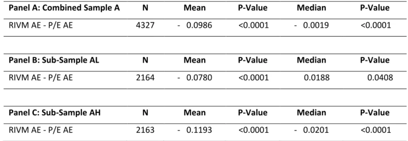
Subsequently, it is pertinent to understand if the models are equally inaccurate. To this end, the newly generated variable DIFFAE portrays the difference between the absolute errors of the RIVM and P/E.
𝐷𝐼𝐹𝐹𝐴𝐸 = 𝐴𝐸𝑉𝐴𝐿𝑅𝐼𝑉𝑀− 𝐴𝐵𝑆𝐸𝑅𝑅𝑂𝑅𝑃𝐸 (38) Based on the following hypothesis tests:
Table 10 – Test of Equality of Valuation Models
Panel A: Combined Sample A N Mean P-Value Median P-Value
RIVM AE - P/E AE 4327 - 0.0986 <0.0001 - 0.0019 <0.0001
Panel B: Sub-Sample AL N Mean P-Value Median P-Value
RIVM AE - P/E AE 2164 - 0.0780 <0.0001 0.0188 0.0408
Panel C: Sub-Sample AH N Mean P-Value Median P-Value
RIVM AE - P/E AE 2163 - 0.1193 <0.0001 - 0.0201 <0.0001
From the table above, we conclude that the null hypothesis is rejected for both mean and median at the previously specified 5% significance level. The RIVM appears to be more accurate in general but its performance is particularly outstanding for the high proportion of intangibles sub-sample IH in comparison to the P/E. In turn, the differences in the medians are evidently less substantial.
It may now be reasonable to argue that the RIVM is more appropriate to valuate firms with a high proportion of intangibles.
24 Wilcoxon signed ranked is the median p-value.
Wilcoxon Signed Rank24
𝐻0: 𝑀𝑒𝑑𝑖𝑎𝑛 𝐷𝐼𝐹𝐹_𝐴𝐸 = 0 𝐻1: 𝑀𝑒𝑑𝑖𝑎𝑛 𝐷𝐼𝐹𝐹_𝐴𝐸 ≠ 0
T-Test
𝐻0: 𝑀𝑒𝑎𝑛 𝐷𝐼𝐹𝐹_𝐴𝐸 = 0 𝐻1: 𝑀𝑒𝑎𝑛 𝐷𝐼𝐹𝐹_𝐴𝐸 ≠ 0
35
3.5.1.2.4 Equality of Value Estimates across Fiscal Years and SIC3 Groups
To verify if there is mean equality across fiscal years and industries, an analysis of variance (ANOVA) covering the generic sample and its sub samples was conducted. Below follow the tests’ hypotheses where m stands for the valuation models, j for the samples, f for fiscal year and s for the SIC3 groups.
As seen on the panels of Table 11, the null hypothesis could not be rejected only in the case of the P/E signed error across Fiscal Years in Sample IL (yet at 5%). For all the other cases, at least one mean value estimate is different.
It is then safe to admit that value estimates differ depending on fiscal year and SIC3 group.
𝐻0: 𝑀𝑒𝑎𝑛 𝑉𝑎𝑙𝑢𝑒 𝐸𝑠𝑡𝑖𝑚𝑎𝑡𝑒𝑚,𝑗,2006= ⋯ = 𝑀𝑒𝑎𝑛 𝑉𝑎𝑙𝑢𝑒 𝐸𝑠𝑡𝑖𝑚𝑎𝑡𝑒𝑚,𝑗,𝑓 𝐻1: 𝐴𝑡 𝑙𝑒𝑎𝑠𝑡 𝑜𝑛𝑒 𝑚𝑒𝑎𝑛 𝑣𝑎𝑙𝑢𝑒 𝑒𝑠𝑡𝑖𝑚𝑎𝑡𝑒 𝑖𝑠 𝑑𝑖𝑓𝑓𝑒𝑟𝑒𝑛𝑡
𝐻0: 𝑀𝑒𝑎𝑛 𝑉𝑎𝑙𝑢𝑒 𝐸𝑠𝑡𝑖𝑚𝑎𝑡𝑒𝑚,𝑗,104= ⋯ = 𝑀𝑒𝑎𝑛 𝑉𝑎𝑙𝑢𝑒 𝐸𝑠𝑡𝑖𝑚𝑎𝑡𝑒𝑚,𝑗,𝑠 𝐻1: 𝐴𝑡 𝑙𝑒𝑎𝑠𝑡 𝑜𝑛𝑒 𝑚𝑒𝑎𝑛 𝑣𝑎𝑙𝑢𝑒 𝑒𝑠𝑡𝑖𝑚𝑎𝑡𝑒 𝑖𝑠 𝑑𝑖𝑓𝑓𝑒𝑟𝑒𝑛𝑡
36 Table 11 – Test on the Equality of Means Across Fiscal Years and SIC3 Groups
Panel I: Combined Sample I N P-Value
Across Fiscal Years
P/E Signed Error 4327 0.0113
P/E Absolute Error 4327 <0.0001
RIVM Signed Error 4327 <0.0001
RIVM Absolute Error 4327 <0.0001
Across SIC3 Groups
P/E Signed Error 4327 <0.0001
P/E Absolute Error 4327 <0.0001
RIVM Signed Error 4327 <0.0001
RIVM Absolute Error 4327 <0.0001
Panel II: Sub-Sample IL N P-Value
Across Fiscal Years
P/E Signed Error 2164 0.0599
P/E Absolute Error 2164 0.0296
RIVM Signed Error 2164 <0.0001
RIVM Absolute Error 2164 0.0032
Across SIC3 Groups
P/E Signed Error 2164 <0.0001
P/E Absolute Error 2164 <0.0001
RIVM Signed Error 2164 <0.0001
RIVM Absolute Error 2164 <0.0001
Panel III: Sub-Sample IH N P-Value
Across Fiscal Years
P/E Signed Error 2163 0.006
P/E Absolute Error 2163 0.0002
RIVM Signed Error 2163 <0.0001
RIVM Absolute Error 2163 <0.0001
Across SIC3 Groups
P/E Signed Error 2163 <0.0001
P/E Absolute Error 2163 <0.0001
RIVM Signed Error 2163 <0.0001
37
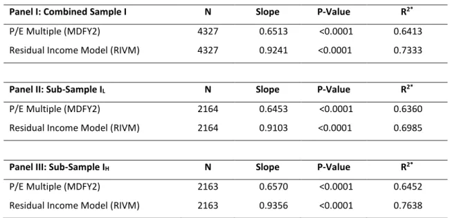
3.5.2 Explanatory Power of Valuation Models
In order to understand the extent to which the models are able to explain market price, an Ordinary Least Squares (OLS) regression will be constructed where the market price (P4) depends on the value estimate of each model25.
𝑃4𝑖𝑗 = 𝛼 + 𝛽 × 𝑉𝑎𝑙𝑢𝑒 𝐸𝑠𝑡𝑖𝑚𝑎𝑡𝑒𝑖𝑗+ 𝜀𝑖𝑗26 (39)
Table 12 – Regression Results
Panel I: Combined Sample I N Slope P-Value R2*
P/E Multiple (MDFY2) 4327 0.6513 <0.0001 0.6413 Residual Income Model (RIVM) 4327 0.9241 <0.0001 0.7333
Panel II: Sub-Sample IL N Slope P-Value R2*
P/E Multiple (MDFY2) 2164 0.6453 <0.0001 0.6360 Residual Income Model (RIVM) 2164 0.9103 <0.0001 0.6985
Panel III: Sub-Sample IH N Slope P-Value R2*
P/E Multiple (MDFY2) 2163 0.6570 <0.0001 0.6452 Residual Income Model (RIVM) 2163 0.9356 <0.0001 0.7638
The adjusted Rsquared (R2*) which reflects the suitability of the model to explain the market
price of the stock is higher for the RIVM than for the P/E. Indeed, RIVM is able to explain more than 75% of the stock’s market price of firms with high PINTAN.
Despite both models showing a fair explanatory power, the differences between P/E multiple and RIVM are patent, though less notably for sub-sample IL.
These results are consistent to what has been seen previously in this paper regarding the superior precision of RIVM in valuing firms with a high proportion of intangibles.
25 VAL
RIM and VHMEANPE
26 Where i represents each observation and j sub-samples I, I L and IH