Mapping dynamic environments using Markov
random field models
Hongjun Li
1, Miguel Bar˜ao
2and Lu´ıs Rato
1 1Department of Informatics, University of Evora, Evora, Portugal2Research Centre for Mathematics and Applications, University of Evora, Evora, Portugal [email protected], [email protected], [email protected]
Abstract—This paper focuses on dynamic environments for mobile robots and proposes a new mapping method combining hidden Markov models (HMMs) and Markov random fields (MRFs). Grid cells are used to represent the dynamic en-vironment. The state change of every grid cell is modelled by an HMM with an unknown transition matrix. MRFs are applied to consider the dependence between different transition matrices. The unknown parameters are learnt from not only the corresponding observations but also its neighbours. Given the dependence, parameter maps are smooth. Expectation Maximum (EM) is applied to obtain the best parameters from observations. Finally, a simulation is done to evaluate the proposed method.
Keywords—Hidden Markov models, Grid map, Markov random fields.
I. INTRODUCTION
The earlier research for mobile robots is developed under the static environment assumption. However, in real environ-ments, there are dynamic objects such as people and doors. Dynamic objects move randomly and it is not easy to know their next positions precisely. Object tracking is to estimate the positions and velocities of dynamic objects. The estimation provides instant information of dynamic objects and the robot can plan its next step in order to avoid collisions.
Another representative model for dynamic environments is HMM [1]. HMM is applied to model the dynamic environ-ments in [2]. The map is divided into grid cells [3] and an HMM is applied to model every grid cell. Every grid cell has two possible states: occupied and free. The state change of one grid cell is represented by a transition matrix. One grid cell may also be observed occupied or free. In addition, the grid cell is unknown when it is outside the measurement. Given the measurements obtained by sensors, the transition matrix can be learnt. In [4], there are three possible observations: true, false and not observable. However, the underlying possible states are extended and consist of seven components: true, false, unknown, dynamic, falsely false, false true, falsely true/false. The last three are used to deal with wrong observations. HMM is applied to classify dynamic objects such as adults, cars and dogs [5]. The transition probabilities are learnt from a clustered exemplar set and can be used to classify tracks of different objects in a Bayesian filtering framework. The dynamic maps based on HMM are used to do lifelong localization task in [6] and simultaneous localization and mapping in [7]. The
This work was supported by EACEA under the Erasmus Mundus Action 2, Strand 1 project LEADER - Links in Europe and Asia for engineering, eDucation, Enterprise and Research exchanges.
observations of neighbour cells in the previous time step are considered in [8] and it is modelled as an input-output hidden Markov model (IOHMM) [9]. The current state of one grid cell depends on not only its previous state but also the previous observations of its neighbours. In this manner, the spatial correlation is considered. The Explicit-state-Duration Hidden Markov Model (EDHMM) is applied to differentiate the dynamic cells from static environment [10]. The duration between two states is variable.
In this paper, we propose a new mapping method for dynamic environments, which combines HMMs and MRFs. The dynamic environment is divided into grid cells and an HMM is also applied to model every grid cell. The transition matrices in HMMs are unknown parameters. The dependence between different transition matrices is considered by MRFs to ensure smooth estimation. HMMs are introduced in Section II. One grid cell is associated with two parameters and one map is represented by two parameter maps. In Section III, the proposed method is presented under the assumption that two parameter maps are independent. Two parameter maps are regarded as two independent MRFs. The MRF model is built in Section III-A. EM for the MRF model is applied to learn the parameters in Section III-B. The simulation is described in Section IV.
II. HMMS FOR DYNAMIC ENVIRONMENTS
The map is divided into many grid cells and every grid cell at coordinate 𝑐 have two possible states: occupied and free, which are denoted 𝑠1 and 𝑠2. In dynamic environments, the states of some grid cells may change over time. The changes can be modelled as Markov chains. A Markov chain can be specified by a transition matrix as
𝐴𝑐= [ 𝑎𝑐 11 1 − 𝑎𝑐11 1 − 𝑎𝑐 22 𝑎𝑐22 ] , (1)
where 𝑎𝑐11 = 𝑝(𝑚𝑡+1𝑐 = 𝑠1 ∣ 𝑚𝑡𝑐 = 𝑠1) represents the probability of state staying occupied from time 𝑡 to time 𝑡 + 1 and 𝑎𝑐
22 = 𝑝(𝑚𝑡+1𝑐 = 𝑠2 ∣ 𝑚𝑡𝑐 = 𝑠2) represents the probability of state staying free. In our work, a laser sensor is used to precept the environment. Because of the uncertainty of the sensor, the state cannot be measured precisely. Following along a laser beam in the measurement direction, the grid cells are free at least until the measured distance. At the end of the measurement range, the cell is occupied. When the measurement range is the maximum range of laser beam, all the grid cells covered by the laser beam are free. One grid
cell is not observed all the time. The observation model can be specified by 𝐵 = [ 𝑝(𝑧 ∣ 𝑚𝑡 𝑐= 𝑠1) 0 0 𝑝(𝑧 ∣ 𝑚𝑡 𝑐= 𝑠2) ] , (2) where 𝑧 ∈ {𝑜𝑐𝑐𝑢𝑝𝑖𝑒𝑑, 𝑓𝑟𝑒𝑒, 𝑢𝑛𝑜𝑏𝑠𝑒𝑟𝑣𝑒𝑑} [2].
The observation model is known. In order to estimate the transition matrix, the initial probabilities𝜌𝑐1= 𝑝(𝑚0𝑐 = 𝑠1) and 𝜌𝑐
2 = 𝑝(𝑚0𝑐 = 𝑠2) are required. The parameters for an HMM are denoted 𝜃𝑐 = {𝑎𝑐11, 𝑎𝑐22, 𝜌1}. Assume the observation sequence is 𝑂𝑐 = {𝑦𝑐0, 𝑦1𝑐, ⋅ ⋅ ⋅ , 𝑦𝜁𝑐} and a underlying state sequence ℳ𝑐. The joint distribution of observations and an underlying state sequence is
𝑝(𝑂𝑐, ℳ𝑐∣ 𝜃𝑐) = 𝑝(𝑚0 𝑐)𝑝(𝑧0∣ 𝑚0𝑐) 𝜁 ∏ 𝑡=1 𝑝(𝑚𝑡 𝑐 ∣ 𝑚𝑡−1𝑐 ) 𝜁 ∏ 𝑡=1 𝑝(𝑦𝑡∣ 𝑚𝑡 𝑐), (3)
The parameters can be estimated by maximum likelihood as ˆ𝜃𝑐= arg max
𝜃
∑
ℳ𝑐
𝑝(𝑂𝑐, ℳ𝑐∣ 𝜃𝑐). (4)
However, it is not feasible to maximize the likelihood directly. Baum-Welch algorithm can be applied to estimate the param-eters by maximizing a 𝑄 function, which is given as
𝑄(𝜃𝑐, 𝜃(𝑘)𝑐 ) = ∑ ℳ𝑐 𝑝(ℳ𝑐∣ 𝑂𝑐, 𝜃(𝑘)𝑐 )log𝑝(ℳ𝑐, 𝑂𝑐 ∣ 𝜃𝑐) =∑ ℳ𝑐 𝑝(ℳ𝑐∣ 𝑂𝑐, 𝜃𝑐(𝑘)) (log𝑝(𝑂𝑐∣ ℳ𝑐, 𝜃𝑐) + log𝑝(ℳ𝑐∣ 𝜃𝑐)) =∑ ℳ𝑐 𝑝(ℳ𝑐∣ 𝑂𝑐, 𝜃𝑐(𝑘))log𝑝(𝑂𝑐 ∣ ℳ𝑐, 𝜃𝑐) +∑ ℳ𝑐 𝑝(ℳ𝑐∣ 𝑂𝑐, 𝜃(𝑘)𝑐 )log𝑝(ℳ𝑐∣ 𝜃𝑐). (5)
Given the state sequence ℳ𝑐, the observation sequence 𝑂𝑐 does no depend on the parameters 𝜃𝑐. 𝑝(𝑂𝑐 ∣ ℳ𝑐, 𝜃𝑐) can
be rewritten as 𝑝(𝑂𝑐 ∣ ℳ𝑐), which can be derived from the observation probabilities. Because the observation probabilities are known, the first item is a constant in (5). Focus on the second one, we can obtain
∑ ℳ𝑐 𝑝(ℳ𝑐 ∣ 𝑂𝑐, 𝜃(𝑘)𝑐 )log𝑝(ℳ𝑐 ∣ 𝜃𝑐) = 2 ∑ 𝑖=1 𝛾𝑐 𝑖(0)log𝜌𝑐𝑖 + ∑ 𝑡 2 ∑ 𝑖=1 𝜉𝑐 1𝑖(𝑡)log𝑎𝑐1𝑖+ ∑ 𝑡 2 ∑ 𝑖=1 𝜉𝑐 2𝑖(𝑡)log𝑎𝑐2𝑖 = 𝑓(𝜌𝑐 1) + 𝑓(𝑎𝑐11) + 𝑓(𝑎𝑐22), (6) where 𝑓(𝜌𝑐 1) = 2 ∑ 𝑖=1 𝛾𝑐 𝑖(0)log𝜌𝑐𝑖 = 𝛾𝑐 1(0)log𝜌𝑐1+ 𝛾2𝑐(0)log(1 − 𝜌𝑐1), (7) 𝑓(𝑎𝑐 11) = ∑ 𝑡 2 ∑ 𝑖=1 𝜉𝑐 1𝑖(𝑡)log𝑎𝑐1𝑖 =∑ 𝑡 𝜉𝑐 11(𝑡)log𝑎𝑐11+ ∑ 𝑡 𝜉𝑐 12(𝑡)log(1 − 𝑎𝑐11), (8) 𝑓(𝑎𝑐 22) = ∑ 𝑡 2 ∑ 𝑖=1 𝜉𝑐 2𝑖(𝑡)log𝑎𝑐2𝑖 =∑ 𝑡 𝜉𝑐 21(𝑡)log(1 − 𝑎𝑐22) + ∑ 𝑡 𝜉𝑐 22(𝑡)log𝑎𝑐22, (9) and𝛾𝑖𝑐(𝑡) = 𝑝(𝑚𝑡𝑐 = 𝑠𝑖∣ 𝑂𝑐, 𝜃𝑐(𝑘)) is the probability of being
in state 𝑠𝑖 at time 𝑡 given the observed sequence 𝑂𝑐 and the parameters 𝜃𝑐(𝑘), 𝜉𝑐𝑖𝑗(𝑡) = 𝑝(𝑚𝑡𝑐 = 𝑠𝑖, 𝑚𝑡+1𝑐 = 𝑠𝑗 ∣ 𝑂𝑐, 𝜃(𝑘)𝑐 )
is the probability of being in state 𝑠𝑖 at time 𝑡 and state 𝑠𝑗 at time𝑡+1 given the observed sequence 𝑂𝑐and parameters𝜃(𝑘)𝑐 . 𝛾𝑐
𝑖(𝑡) and 𝜉𝑖𝑗𝑐(𝑡) can be computed as the forward process and
backward process in Baum-Welch algorithm. The parameters can be updated as 𝜌𝑐(𝑘+1)𝑖 = 𝛾𝑐 𝑖(0), (10) 𝑎𝑐(𝑘+1)𝑖𝑗 = ∑𝜁 𝑡=1𝜉𝑖𝑗𝑐(𝑡) ∑𝜁 𝑡=1𝛾𝑖𝑐(𝑡) . (11)
III. PROPOSED METHOD A. The MRF model
The set of 𝑎𝑐11 and𝑎𝑐22 for all the grid cells are denoted
𝑨 = (𝒂1, 𝒂2), where 𝒂1 = [⋅ ⋅ ⋅ , 𝑎𝑐11, ⋅ ⋅ ⋅ ]T and 𝒂2 = [⋅ ⋅ ⋅ , 𝑎𝑐
22, ⋅ ⋅ ⋅ ]T. 𝒂1 and 𝒂2 are assumed to be independent. The prior distribution can be factorized as
𝑝(𝑨) = 𝑝(𝒂1)𝑝(𝒂2). (12) The dependence between different 𝑎11 and the dependence between different 𝑎22 are considered individually.𝒂1is taken as an example to show how to formulate the dependence. The log odds form of𝑎𝑐11 is defined as
𝑙𝑐 𝑎11= log 𝑎𝑐 11 1 − 𝑎𝑐 11. (13)
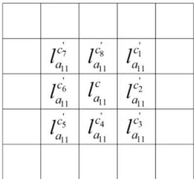
Assume the vector of all the 𝑙𝑎𝑐11 is regarded as an MRF and denoted𝑙𝑎1 = [⋅ ⋅ ⋅ , 𝑙𝑐𝑎11, ⋅ ⋅ ⋅ ]T. A second-order neighbourhood system in this MRF, which includes the diagonal grid cells, is shown as Figure 1. Every random variable 𝑙𝑐𝑎11 has eight neighbours denoted 𝑙𝑐𝑎11′ .
Fig. 1: A second-order neighbourhood system in an MRF
A clique 𝐶 is defined as a subset of variables that are neighbours to one another. The pair-variable cliques are shown in Figure 2. The collection of the pair-variable cliques is denoted 𝐶2. In one second-order neighbourhood, there are eight pair-variable cliques.
Fig. 2: Pair-variable cliques in second-order neighbourhood system
Only the pair-variable cliques in the second-order neigh-bourhood systems are considered. The prior probability is
𝑝(𝑙𝑎1) = 1 𝑍exp(− 1 𝒯 ∑ 𝐶∈𝐶2 𝑉𝐶(𝑙𝑎1)), (14) where 𝑍 =∑ 𝑙𝑎1 exp(−𝒯1 ∑ 𝐶∈𝐶2 𝑉𝐶(𝑙𝑎1)), (15)
𝒯 is the temperature, 𝑉𝐶(𝑙𝑎1) is the clique potential and
defined as
𝑉𝐶(𝑙𝑎1) = (𝑙𝑐𝑎11− 𝑙 𝑐′
𝑎11)
2. (16)
Expand these clique potentials, the sum in (14) is quadratic. The prior can be rewritten as
𝑝(𝑙) =𝑍1exp(−𝒯2𝑙T
𝑎1𝒜𝑙𝑎1). (17)
The prior distribution 𝑝(𝒂1) is 𝑝(𝒂1) =𝑍1exp ( −𝒯1𝑈(𝒂1) ) , (18) where 𝑈(𝒂1) = 2(log1 − 𝒂𝒂1 1) T𝒜log 𝒂1 1 − 𝒂1. (19)
1 is a column of ones. Similarly, the log odds form of 𝑎𝑐 22 is defined as 𝑙𝑐 𝑎22= log 𝑎𝑐 22 1 − 𝑎𝑐 22. (20) Assume the vector of all the 𝑙𝑐𝑎22 is also regarded as an MRF and denoted 𝑙𝑎2= [⋅ ⋅ ⋅ , 𝑙𝑐𝑎22, ⋅ ⋅ ⋅ ]T.𝑝(𝒂2) is given as
𝑝(𝒂2) =𝑍1exp ( −𝒯1𝑈(𝒂2) ) , (21) where 𝑈(𝒂2) = 2(log1 − 𝒂𝒂2 2) T𝒜log 𝒂2 1 − 𝒂2. (22)
𝒂1and𝒂2have the same configuration space. The normalizers in two different distributions are the same as𝑍.
The coordinate set of observed grid cells is denoted ℐ and the observation set 𝑂 = {𝑂𝑐} (𝑐 ∈ ℐ) consists all the
observation sequences𝑂𝑐 of observed grid cells. A underlying configuration sequence is denotedℳ = {ℳ𝑐} (𝑐 ∈ ℐ), which consists of all the underlying state sequences of observed grid cells. In probabilistic form, the likelihood is 𝑝(𝑂 ∣ 𝑨). The joint probability 𝑝(𝑂, ℳ ∣ 𝑨) is
𝑝(𝑂, ℳ ∣ 𝑨) = 𝑝(𝑂 ∣ ℳ, 𝑨)𝑝(ℳ ∣ 𝑨). (23) Assume all the observation sequences are dependent of each other, it is rewritten as
𝑝(𝑂, ℳ ∣ 𝑨) =∏ 𝑐∈ℐ
𝑝(𝑂𝑐∣ ℳ𝑐, 𝐴𝑐)𝑝(ℳ𝑐 ∣ 𝐴𝑐), (24)
where 𝑝(𝑂𝑐 ∣ ℳ𝑐, 𝐴𝑐) is the same as 𝑝(𝑂𝑐 ∣ ℳ𝑐, 𝜃𝑐) and 𝑝(ℳ𝑐 ∣ 𝐴𝑐) is the same as 𝑝(ℳ𝑐∣ 𝜃𝑐). For convenience, 𝐴𝑐
is used instead. The likelihood can be given as 𝑝(𝑂 ∣ 𝑨) =∑
ℳ
𝑝(𝑂, ℳ ∣ 𝑨) (25)
Based on Bayes rule, the posterior distribution is
𝑝(𝑨 ∣ 𝑂) = 𝑝(𝑂 ∣ 𝑨)𝑝(𝑨)𝑝(𝑂) , (26) where 𝑝(𝑂) is a constant.
B. EM
Maximizing𝑝(𝑨 ∣ 𝑂), the best estimation can be obtained. Equivalently we need to maximizing
𝑝(𝑂, 𝑨) = 𝑝(𝑂 ∣ 𝑨)𝑝(𝑨). (27) This problem is similar to the HMM without prior and it is not possible to search the maximum directly. EM algorithm is applied to solve this problem. In E step, the𝑄 function is given as 𝑄(𝑨, 𝑨(𝑘)) = 𝐸 ℳ∣𝑂,𝑨(𝑘)log𝑝(ℳ, 𝑂 ∣ 𝑨) + log𝑝(𝑨) = 𝐸ℳ∣𝑂,𝑨(𝑘)log𝑝(𝑂 ∣ ℳ, 𝑨) + 𝐸ℳ∣𝑂,𝑨(𝑘)log𝑝(ℳ ∣ 𝑨) − 2log𝑍 − 1 𝒯𝑈(𝒂1) − 1 𝒯 𝑈(𝒂2). (28)
𝑝(𝑂 ∣ ℳ, 𝑨) can be rewritten as 𝑝(𝑂 ∣ ℳ). The first term andlog𝑍 are constants. Discarding the constant parts gives 𝐸ℳ∣𝑂,𝑨(𝑘)log𝑝(ℳ ∣ 𝑨) − 1 𝒯𝑈(𝒂1) − 1 𝒯 𝑈(𝒂2) =∑ ℳ 𝑝(ℳ ∣ 𝑂, 𝑨(𝑘))∑ 𝑐∈ℐ log𝑝(ℳ𝑐 ∣ 𝐴𝑐) −𝒯1𝑈(𝒂1) −𝒯1𝑈(𝒂2) =∑ 𝑐∈ℐ ∑ ℳ 𝑝(ℳ ∣ 𝑂, 𝑨(𝑘))log𝑝(ℳ 𝑐∣ 𝐴𝑐) −𝒯1𝑈(𝒂1) −𝒯1𝑈(𝒂2) =∑ 𝑐∈ℐ ∑ ℳ𝑐 𝑝(ℳ𝑐∣ 𝑂, 𝜃(𝑘)𝑐 )log𝑝(ℳ𝑐 ∣ 𝐴𝑐) −𝒯1𝑈(𝒂1) −𝒯1𝑈(𝒂2). (29) Based on (6), this expectation is rewritten as
𝐸ℳ∣𝑂,𝑨(𝑘)log𝑝(ℳ ∣ 𝑨) − 1 𝒯 𝑈(𝒂1) − 1 𝒯𝑈(𝒂2) =∑ 𝑐∈ℐ 𝑓(𝜌𝑐 1) + ∑ 𝑐∈ℐ 𝑓(𝑎𝑐 11) + ∑ 𝑐∈ℐ 𝑓(𝑎𝑐 22) − 2𝑈(𝒂1) − 2𝑈(𝒂2) = 𝑓(𝝆1) + 𝑓(𝒂1) + 𝑓(𝒂2), (30)
where the set of initial occupancy probabilities of observed grid cells is denoted 𝝆1 = [⋅ ⋅ ⋅ , 𝜌𝑐1, ⋅ ⋅ ⋅ ]T (𝑐 ∈ ℐ). The three functions𝑓(𝝆1), 𝑓(𝒂1) and 𝑓(𝒂2) are defined as
𝑓(𝝆1) =∑ 𝑐∈ℐ 𝑓(𝜌𝑐 1) = 𝜸1log𝝆1+ 𝜸2log(1 − 𝝆1), (31) 𝑓(𝒂1) =∑ 𝑐 𝑓(𝑎𝑐 11) −𝒯1𝑈(𝒂1) = 𝝃11log𝒂11+ 𝝃12log(1 − 𝒂1) −𝒯2(log1 − 𝒂𝒂1 1) T𝒜log 𝒂1 1 − 𝒂1, (32)
𝑓(𝒂2) =∑ 𝑐 𝑓(𝑎𝑐 2) −𝒯1𝑈(𝒂2) = 𝝃22log𝒂2+ 𝝃21log(1 − 𝒂2) −𝒯2(log1 − 𝒂𝒂2 2) T𝒜log 𝒂2 1 − 𝒂2, (33) 𝜸𝑖 = [⋅ ⋅ ⋅ , 𝛾𝑖𝑐(0), ⋅ ⋅ ⋅ ] and 𝝃𝑖𝑗 = [⋅ ⋅ ⋅ ,∑𝑡𝜉𝑖𝑗𝑐(𝑡), ⋅ ⋅ ⋅ ]. In (32)
and (33), 𝑐 is not limited in ℐ. For unobserved grid cells, the corresponding elements in𝝃𝑖𝑗 are set to 0. The derivatives of 𝑄(𝜽, 𝜽(𝑘)) with respect to 𝝆
1,𝒂1and𝒂2are individually given as d d𝝆1𝑓(𝝆1) = 𝜸 T 1 ⊘ 𝝆1− 𝜸2T⊘ (1 − 𝝆1), (34) d d𝒂1𝑓(𝒂1) =𝝃 T 11⊘ 𝒂1− 𝝃T12⊘ (1 − 𝒂1) − 4 𝒯 𝒜(log 𝒂1 1 − 𝒂1) ⊙ 1 𝒂1⊙ (1 − 𝒂1), (35) d d𝒂2𝑓(𝒂2) =𝝃 T 22⊘ 𝒂2− 𝝃T21⊘ (1 − 𝒂2) −𝒯4𝒜(log1 − 𝒂𝒂2 2) ⊙ 1 𝒂2⊙ (1 − 𝒂2), (36) where ⊘ is the elementwise division and ⊙ is Hadamard product. The best estimation of 𝝆1 is
𝝆1= 𝜸1T. (37)
It is not easy to maximize𝑓(𝒂1) and 𝑓(𝒂2) and a line search method [11] is used to maximize𝑓(𝒂1) and 𝑓(𝒂2) and obtain the best estimation of parameters in range (0,1).
IV. SIMULATION
The true map is shown as Figure 3(a). There are 4 square dynamic objects. They have different changing frequencies and their states keep for Δ𝑡/3, 2Δ𝑡, 3Δ𝑡, 7Δ𝑡. The walls on the left are static. The speed is 3 grid cells per 𝛿𝑡. At a position, there are four measurement directions:±𝜋/2 and ±𝜋/4. They are relative to the robot direction. The maximum range is 8 grid cells. The robot runs near the dashed line randomly 20 loops. The trajectory is shown as Figure 3(b).
(a) Simulated map (b) Trajectory
Fig. 3: The simulated map and the trajectory
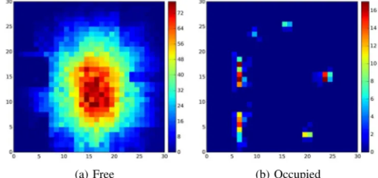
Figure 4(a) represents the times the grid cells are observed. The blue parts are not observed. Figure 4 represents the times
the grid cells are observed free. The free space is observed more than once during one loop. Figure 4(b) represents the times the grid cells are observed occupied. Because of the noise of the sensor, the static walls are observed free and the free space around objects are observed occupied sometimes.
(a) Free (b) Occupied
Fig. 4: The times grid cells are observed free or occupied
The initial parameters 𝒂1, 𝒂2, 𝝆1 are 0.5 and 𝒯 = 50. The maximum iteration of optimizing process is 300 and the parameter estimation is shown as Figure 5. In Figure 5(a), the observed free space is estimated with low 𝑎00 and the walls always stay occupied and have high 𝑎00. Dynamic object 1 and 2 change fast and the corresponding estimation is low. Dynamic object 3 and 4 stay occupied for a long time and their 𝑎00 are also high. In Figure 5(b), the free space always stays free and has high𝑎11. The estimations of𝑎11fo the walls, which should be close to 0, are close to 0.4. Because there are fewer free observations for the walls, it is not easy to estimate 𝑎11. Given the dependence, their parameters also learn from their neighbours which have high𝑎11. For the dynamic objects, the one with a high changing frequency has a high estimation of𝑎11. The observed space in the centre has more observations, the parameter converges fast and the corresponding parameter are estimated well. The parameter on the border converges slowly.
(a)𝑎00: occupied to occupied (b)𝑎11: free to free
Fig. 5: Parameter estimation
V. CONCLUSIONS
In this paper, we propose an HMM-based mapping method using MRFs for dynamic environments. An HMM model is built for every grid cell. The MRFs are applied to consider the
dependence between grid cells and the MRF model is built for the whole map. EM algorithm is used to train the HMM parameters. The simulation demonstrates that the proposed method can ensure smooth estimation. However, it takes a long time to estimate the parameters. In the future, we will improve this work to be an online method and implement it in path planning for mobile robots.
REFERENCES
[1] L. R. Rabiner, “A tutorial on hidden markov models and selected applications in speech recognition,” Proceedings of the IEEE, vol. 77, no. 2, pp. 257–286, 1989.
[2] D. Meyer-Delius, M. Beinhofer, and W. Burgard, “Occupancy grid models for robot mapping in changing environments,” in Proceedings
of the Twenty-Sixth AAAI Conference on Artificial Intelligence, 2012.
[3] H. Moravec and A. Elfes, “High resolution maps from wide an-gle sonar,” in Proceedings of the IEEE International Conference on
Robotics and Automation, vol. 2, pp. 116–121, IEEE, 1985.
[4] M. Rapp, K. Dietmayer, M. Hahn, B. Duraisamy, and J. Dickmann, “Hidden markov model-based occupancy grid maps of dynamic en-vironments,” in Proceedings of the 19th International Conference on
Information Fusion (FUSION), pp. 1780–1788, IEEE, 2016.
[5] M. Luber, K. O. Arras, C. Plagemann, and W. Burgard, “Classifying dynamic objects,” Autonomous Robots, vol. 26, no. 2-3, pp. 141–151, 2009.
[6] G. D. Tipaldi, D. Meyer-Delius, and W. Burgard, “Lifelong localization in changing environments,” The International Journal of Robotics
Research, vol. 32, no. 14, pp. 1662–1678, 2013.
[7] C. Bibby and I. Reid, “Simultaneous localisation and mapping in dynamic environments (slamide) with reversible data association,” in
Proceedings of Robotics Science and Systems, vol. 117, p. 118, 2007.
[8] Z. Wang, R. Ambrus, P. Jensfelt, and J. Folkesson, “Modeling motion patterns of dynamic objects by iohmm,” in Proceedings of the IEEE/RSJ
International Conference on Intelligent Robots and Systems, pp. 1832–
1838, IEEE, 2014.
[9] Y. Bengio and P. Frasconi, “An input output hmm architecture,” in
Advances in neural information processing systems, pp. 427–434, 1995.
[10] A. Dadhich, N. Koganti, and T. Shibata, “Modeling occupancy grids using edhmm for dynamic environments,” in Proceedings of the 2015
Conference on Advances In Robotics, p. 60, ACM, 2015.
[11] S. Wright and J. Nocedal, “Numerical optimization,” Springer Science, vol. 35, no. 67-68, p. 7, 1999.