Improved adaptive Markov random field based super-resolution mapping for mangrove tree identification

IMPROVED ADAPTIVE MARKOV RANDOM FIELD BASED SUPER-RESOLUTION

MAPPING FOR MANGROVE TREE EXTRACTION

H. Aghighia,c∗, J. Trindera, S. Lima, Y. Tarabalkab

a_{School of Civil and Environmental Engineering, The University of New South Wales, UNSW SYDNEY NSW 2052, Australia} h.aghighi@student.unsw.edu.au, j.trinder@unsw.edu.au, s.lim@unsw.edu.au

b _{Inria Sophia-Antipolis M´editerran´ee, AYIN team, 06902 Sophia Antipolis, France- yuliya.tarabalka@inria.fr} c_{Department of Remote Sensing & GIS, Faculty of Earth science, Shahid Beheshti University, Tehran, Iran}

Commission VIII, WG VIII/8

KEY WORDS:Super-resolution mapping, Markov random field, Mangrove forest

ABSTRACT:

Traditionally, forest tree crowns are extracted using airborne or spaceborne hyper-/multi-spectral remotely sensed images or pan-sharpened images. However, these medium/low spatial resolution images suffer from the mixed pixel problem, and the cost to collect very high resolution image collection is high. Moreover, existing feature extraction techniques cannot extract local patterns from medium/low resolution images. Therefore, super-resolution mapping (SRM) techniques, which generate land-cover maps with finer spatial resolution than the original remotely sensed image, can be beneficial for the extraction of forest trees. The SRM methods can improve the quality of information extraction by combining spectral information and spatial context into image classification prob-lems. In this paper we have improved an adaptive Markov random field approach for super-resolution mapping (MRF-SRM) based on spatially adaptive MRF-SPM to overcome the limitation of equal covariance matrices assumption for all classes. We applied the developed method for mangrove tree identification from multispectral image recorded by QuickBird satellite, where we generated a super-resolution map with the panchromatic image spatial resolution of 0.6 m. Moreover, the performance of the proposed technique is evaluated by employing the simulated image with different covariance matrices for each class. Our experimental results have demon-strated that the new adaptive MRF-SRM method has increased the overall accuracy by 5.1% and the termination conditions of this method were satisfied three times faster when compared to the state-of-the-art methods.

1. INTRODUCTION

Deforestation or removal of forests or trees stands has adverse impacts on the water cycle, ecosystem services, biodiversity, and global biogeochemical cycles, leading to droughts, increased carbon emissions, with consequent impact on climate change [Bagley et al., 2014, Jepma C.J., 2014, Mas et al., 2004]. For instance, deforestation for agricultural purposes in the Brazilian Amazon was an important source of increased annual carbon flux over the period 1989-1998 [Houghton et al., 2000]. Thus, de-forestation and forest degradation in the Brazilian Amazon have been observed using remotely sensed data.

Existing deforestation maps in Brazil were generated from medi-um or low resolution satellite images and do not contains local scale information [Li et al., 2013]. For example, Brazilian Space Agency (INPE) produced the deforestation map for the period of 1988 and 1998 by visual interpretation using Landsat thematic mapper data as well as classification of Landsat multi-spectral scanner (MSS) in 1986 [Houghton et al., 2000]. Another limita-tion with the use of medium and coarse pixel resolulimita-tion images is the mixed pixels problem [Li et al., 2013], which do not enable the application of normal feature extraction techniques to utilize the hyper- and multi-spectral data for extraction of local scale in-formation of features as well as individual tree crowns (ITC). This information plays a dominant role in maintaining biotic diversity data [Clark et al., 2005], forest management, species identifica-tion, gap analysis, and volume and biomass estimations [Jing et al., 2012]. Another example of the limitation of medium spatial resolution images was demonstrated for many parts of Africa, where the ITC were not observable within a 30 m resolution

∗_{Corresponding author.}

Landsat TM images [Houghton, 2005]. In order to solve the mixed pixels problem, soft classification methods can be applied. However, they cannot determine the spatial patterns of a forest within each coarse pixel [Li et al., 2013] and it is not possible to extract theITC.

TheITCdelineation from remote sensing data requires high spa-tial resolution overlapping photographs/imagery derived from aerial cameras [Halounov, 2003], videography, multispectral air-borne or spaceair-borne sensors [Clark et al., 2005] and elevation data derived from laser scanning or by GNSS field measure-ment [Ardila et al., 2011]. Although the extractedITCfrom high resolution data presents more information than medium resolu-tion image, it does not solve the problem caused by low/ medium resolution multispectral imagery. Moreover, acquiring high reso-lution time series data sets for a large area is costly and may be impossible [Li et al., 2013].

extrac-tion within coarse pixels are open challenges.

In this paper, we employed super-resolution mapping (SRM) [Tatem et al., 2002], also called sub-pixel mapping [Verhoeye and De Wulf, 2002] which is a land cover classification tech-nique to produce the classified map at a finer spatial resolution than the original coarse resolution image. The idea ofSRMwas introduced by Atkinson [Atkinson, 1997] to achieve sub-pixel vector boundaries using spatial dependence maximization. In general, spatial dependence means that the neighboring pixels be-long, with the high probability, to the same class as observations further apart [Atkinson, 1991]. Later on, several attempts have been made to utilize this theory and employ a method to tackle theSRMissue. Generally,SRMmethods can be divided into two main categories [Li et al., 2012]: 1) methods which are applied as post-processing algorithms and require soft classification results, and 2) those which can be categorised as a classification and are independent of soft classification methods.

The first approach can be divided into methods based on sub-pixel swapping [Luciani and Chen, 2011, Shen et al., 2009, Thornton et al., 2006,Yong and Bo, 2014]; multiple endmember spectral mix-ture analysis [Powell et al., 2007]; geostatistics [Atkinson et al., 2008, Boucher and Kyriakidis, 2006, Boucher et al., 2008, Qun-ming et al., 2014]; the broad category of spatial attraction [Liguo et al., 2011,Mertens et al., 2006,Mertens et al., 2003a,Ling et al., 2013, Wang et al., 2012]; and those based on utilizing heuristic methods to improve theSRMaccuracy by maximizing the spa-tial dependence and generating the spaspa-tial distribution of land cover within the mixed pixels [Mertens et al., 2003b, Tatem et al., 2001, Zhang et al., 2008, Zhong and Zhang, 2013]. In contrast, the secondSRMapproaches do not rely on the availability of ac-curate class boundaries nor a sub-pixel classified map derived by another method [Kasetkasem et al., 2005].

In this paper, we consider the second category for defining con-textualSRM, which was proposed by [Kasetkasem et al., 2005], and employs Markov random field (MRF) because of its suit-ability to represent the spatial dependence between pixels. This method was developed based on three main assumptions: the pix-els of the fine spatial resolution image are pure,SRMsatisfies the MRFproperties, and the pixel intensities for each class in the fine resolution image are normally distributed. In contrast to the first SRMtype, referred to above the results of this method does not rely on the availability of accurate class boundaries nor a sub-pixel classified map derived by another method [Kasetkasem et al., 2005].

In this paper we adoptSRM described in [Tolpekin and Stein, 2009] and the spatially adaptiveMRF-SPM proposed in [Li et al., 2012] both of which have proved to work well on simulated Gaussian distributed multispectral images. These methods were developed based on equal covariance matrix between the classes. The first novelty of this work consists in employing the proposed method for theITCmapping in the mangrove forests. The sec-ond novelty of this work is that it utilizes multispectral QuickBird images with a resolution of 2.4 m, instead of the synthetic image used by [Tolpekin and Stein, 2009,Li et al., 2012], to produce the mangrove forest map at the panchromatic imagery spatial resolu-tion of 0.6 m. Finally, we have attempted to overcome the limi-tation of the equal covariance matrix assumption between classes used by [Tolpekin and Stein, 2009, Li et al., 2012].

The outline of this paper is as follows: Section 2. introduces the basic ofMRF-SRMframe work and explicitly explains the frame work of improved adaptiveMRF-SRM. The data description and the experimental results are presented and discussed in Section 3. Finally, conclusions are drawn in Section 4.

2. PROPOSED METHOD

In the development of MRF based SRM framework, we denote an image byY={Y_i∈RB_{,i=1,2, . . . ,m}, whereBis a number} of spectral channels, andm=N1×N2is a number of pixels in an image. The spatial resolution of imageY is denoted as R; therefore each pixelY_irepresents a square area of sizeR2on the ground. It is assumed that the spectral intensity of each pixel Y_i depends on a corresponding unobserved pixel label inL=

ℓj,j=1,2, . . . ,m [Bouman and Shapiro, 1994], where, each

ℓjtakes its value from a finite set ofMthematic classes of interest Ω={ω1,ω2, . . . ,ωM}. Although imageY was captured by an airborne or spaceborne sensor, we assume that this image was generated by degradation of a not directly observed image (X) with the same number of spectral bands and spatial resolution r. We assume that every pixel ofXis pure and can be assigned to a unique class [Tolpekin and Stein, 2009]. It is also assumed that the spectral intensities of the pixels ofXandYwhich belong to the same class, are spatially uncorrelated [Tolpekin and Stein, 2009].

The ratio between the coarse pixel spatial resolution (R) and fine pixel spatial resolution (r) image is called the scale factor (S=

R/r) and is assumed to be an integer value [Tolpekin and Stein, 2009]. Hence, each coarse pixel of Y consists ofS2pixels ofX and the corresponding positions of fine pixels withinY_{ican be} indexed byxk|i, wherek=1,2, . . . ,S2. By excluding the partial overlaps between the coarse and fine pixels, the relationship be-tween each coarse pixel ofYand its corresponding finer pixels of Xcan be established as follows [Li et al., 2012]:

Y_i= 1

S2 S2

∑

k=1

xk|i (1)

2.1 MRF-SRM

The aim ofSRMis to produce a classified mapCSRM at a finer spatial resolution (r), the same asX, from a coarse resolution im-age (Y) [Tolpekin and Stein, 2009]. For this reason we employed the Bayes’ rule:

p(CSRM|Y)∝p(Y|CSRM)p(CSRM) (2)

wherep(CSRM|Y)is the posterior probability of the classifiedSR map,p(Y|CSRM)is the class-conditional probability andp(CSRM) is the prior probability distribution for theSRmapCSRM. The op-timal classifiedSRmapC∗_SRMgiven the imageYcan be generated by solving the maximization problem for the a posteriori proba-bility (MAP) decision rule (2):

CSRM∗ =argmax CSRM

{p(CSRM|Y)}=argmax CSRM

{p(Y|CSRM)p(CSRM)}

(3) According to the complexity of (3) which involves the optimiza-tion of a global distribuoptimiza-tion of the image and due to the equiva-lence ofMRFand Gibbs random field, this optimization can be resolved by minimizing the sum of local posterior energies, as proposed in [Tolpekin and Stein, 2009]:

U(CSRM|Y) =U(Y|CSRM) +U(CSRM) (4)

labels for neighboring sub-pixels:

U(CSRM) =

∑

k,i

UCSRM

a_k|i=

∑

k,i

∑

al∈N(ak|i)

q×φ(al)×

1−δCSRM

ak|i

,CSRM(al)

(5)

Here,UCSRM

a_k|iis the local spatial energy of the sub-pixel

ak|i andCSRM

ak|i

is the class label of sub-pixelak|iwithin a coarse pixelY_i, andCSRM(al)is the class label of its surround-ing neighbors. In this equation,δ ℓi, ℓjis the Kronecker delta function,(δ ℓi, ℓj

=1 ifℓi=ℓjandδ ℓi, ℓj

=0 ifℓi6=ℓj),q controls the overall magnitude of weights and consequently the contribution of the spatial energies 0≤q<∞, andφ(al)denotes the weight of contribution from sub-pixel al ∈N

a_k|ito the spatial energy term and can be computed as (6):

φ(al) = 1

η





d

ak|i,al

r   −g (6)

where da_k|i,al

denotes the geometric distance between the sub-pixelak|iand its spatial neighborsal[Li et al., 2012, Makido et al., 2007],ηis the normalization constant so that∑_l∈N(a

k|i)η(al)

=1, and the power law indexgis usually set asg=1 [Li et al., 2012]. The spectral energy termU(Y|CSRM)can be expressed as:

USpectral(Y|CSRM) =

∑

i,k

UY_i|CSRM

ak|i

=

_∑

i,k

1

2(Yi−µi) ′

Σ_i−1_(Y i−µi) +

1 2ln|Σi|

(7)

whereY_{iis the spectral vector of the coarse pixeli, assumed to be} normally distributed with meanµiand covarianceΣi. Bothµiand Σ_iare dependent on the pixel composition and can be computed using [Tolpekin and Stein, 2009]:

µi= M

∑

α=1

θαiµα (8)

Σi= M

∑

α=1

θαiΣα (9)

whereθαiis the proportion of the classωα in the composition

of coarse pixelY_{i, such that} M_∑ α=1

θαi=1, andµαandΣαare the

mean and covariance of the classωα, which are estimated using the sufficient number of pure training pixels [Kasetkasem et al., 2005]. By substituting (5, 7) in (4), we can write (4) as:

U(CSRM|Y) =U(Y|CSRM) +q

∑

k,i

∑

al∈N(ak|i)

φ(al)×

1−δCSRM

ak|i

,CSRM(al)

(10)

In order to normalizeU(CSRM|Y), we multiply (10) by 1/(1+q):

U(CSRM|Y)∝ 1

1+qU(Y|CSRM) + q

1+q

∑

_k,i

∑

al∈N(ak|i) φ(al)×

1−δCSRM

ak|i

,CSRM(al)

(11)

In this step we callq/(1+q)smoothing parameter which is de-noted asλ; hence 1/(1+q)can be expressed as 1−λ. As men-tioned in Equation (3), the optimal SR mapC_SRM∗ depends on the maximizing the posterior probability which is similar to min-imization of posterior energyU(CSRM|Y), not the absolute value ofU(CSRM|Y)[Tolpekin and Stein, 2009]; thus, equation (11) can be written as :

U(CSRM|Y) = (1−λ)U(Y|CSRM) +λ

∑

k,i

∑

al∈N(ak|i)

φ(al)×

1−δCSRM

ak|i

,CSRM(al)

(12)

2.2 Adaptive MRF-SRM

According to Equations (5) and (7) the spatial and spectral en-ergies which are required to compute posterior energy in Equa-tion (12) should be computed for each coarse pixel. However, λ in (12) was a fixed value for the entire image by [Tolpekin and Stein, 2009]. Thus, by estimating a smoothing parameter for each coarse pixel using its local contextual information, we can mod-ify theMRF-SRMmodel (12) into an adaptiveMRF-SRM[Li et al., 2012]. For this reason, assume that the class label of a given sub-pixelCSRM

ak|i

=αis assigned to an incorrect class label

CSRM

ak|i

=β within a coarse pixelY_{i. Therefore, based on} (3) we can infer that:

U

CSRM

ak|i

=α|Y_{i≥UCSRMak|i=β|}Y_{i (13)}

If this condition is not corrected, then an incorrect class label will be assigned by theMAPsolution toa_k|i. Substituting the corresponding terms in (13) and solving this inequality equation, we will have changes in the spectral energy∆U_αβspec and in the

spatial energy∆U_αβspat[Tolpekin and Stein, 2009]; where,∆U_αβspec

can be computed using (14) and∆U_αβspatusing (15) [Tolpekin and Stein, 2009, Li et al., 2012].

∆U_αβspec= 1 2

_µ

β−µα

S2

′

Σi−1

_µ

β−µα

S2

(14)

where due to equal covariance matrix assumptionΣ_i= 1/S2

Σ_α [Tolpekin and Stein, 2009] Moreover, they proposed Equation (15) to compute the change in spatial energy∆U_αβspatfrom classα toβ[Tolpekin and Stein, 2009] .

∆U_αβspat=q

∑

al∈N(ak|i)

φ(al) [δ(β,CSRM(al))−δ(α,CSRM(al))]

=qγ (15)

where parameterγis related to the prior energy coefficientφ, the neighbouring window size (W =2S−1) and the configuration of pixel class labelCSRM(al) in theN

ak|i

of a specific im-age [Tolpekin and Stein, 2009]. Furthermore,γfor each pair of classes (αandβ) can be estimated as [Tolpekin and Stein, 2009]:

λ∗= 1 1+_∆Uγspec

αβ

(16)

pixel to compute the mean of spectral energy change ∆U_iSpec within each coarse pixel:

∆U_iSpec= ∑ M−1

α=1∑Mβ=α+1θαiθβi∆U Spec αβ

∑M_α=−₁1∑_βM_=α+1θαiθβi

(17)

Then, they modified (16) as:

λi∗= 1 1+ γ

∆U_iSpec

(18)

Equation (18) computes the smoothing parameter for each coarse pixelY_{i. Hence, this method can be considered as an adaptive} super resolution mapping method. However, it should be noted that the spectra statistics of classes show that the mean and co-variance of classes are different; thus, the maximum likelihood estimation utilizes the likelihood energy (7) to assign a class to a given pixel based on minimum distance [Richards and Jia, 2006]. However, both methods [Tolpekin and Stein, 2009,Li et al., 2012] suffer from the assumption of the same class covariance matrix in Equation (14); thus, they employed the Mahalanobis distance (14) to estimate the spectral energy change from a correct class to an incorrect class label∆U_αβspec. To overcome this limitation, we proposeΣ_αβwhich is the average of covariance matrix of classes αandβ, instead of using the same covariance matrix for all the classes:

Σ_αβ=Σα+Σβ

2 (19)

By employing (19), Equation (14) can be rewritten as (20).

∆U_αβspec= 1 2

_µ

β−µα

S2

′

Σ_αβ−1

_µ

β−µα

S2

(20)

By utilizing (20) instead of (14), our adaptiveMRF-SRMis not dependent on the same covariance matrix which assumed by [Tolpekin and Stein, 2009, Li et al., 2012]. Moreover, it can be applied on a real image with a different covariance matrix for each class to produce aSRmap.

2.3 Optimization and Estimation

In this work, we employed simulated annealing (SA) as a heuris-tic optimization technique to iteratively search for a new solution (see Figure 1). The simulated annealing schedule is based on the following power-law decay function:

Titer=σTiter−1, (21)

whereTiter is the temperature at the iteration numberiter, and

σ∈(0,1)controls the rate of temperature decrease. In the first step of this method, an initialSRmap should be produced. For this reason, we employed a constraint linear spectral unmixing (LSU) method to generate the initial class proportion of each coarse pixel (Figure 3(d)). Then the scale factor and estimated fractional abundance (FAj) results for each coarse pixel were uti-lized to estimate the number of sub-pixelsNSPjfor each class j within a coarse pixelY_i:

NSPj=round

FAj 1/S

, (22)

whereround(•)returns the value of the closest integer. Then, we randomly assign a numberNSPj of sub-pixels within a coarse pixelY_{i: to classℓj. We called the generated map as the initial}

SRmapCInit_SRMak|i

. In the next step, we compute the spectral

energy change∆U_αβspecusing (20) and the mean of spectral change ∆U_ispecusing (17) to estimate the optimal smoothing parameter λ_i∗for each coarse pixel by (18). Then,λ_i∗was used to compute the posterior energy (12) of each coarse pixel. Before starting the iterative steps, some parameters should be defined: the starting iteration number (iterstart=1), maximum number of iterations (itermax), starting temperatureT0=2, the temperatureσ=0.9. The SA is performed until it satisfies the termination conditions: 1)iter≥itermax; 2) less than 0.1% of the sub-pixels are success-fully updated during three consecutive iterations.

In order to utilize the SA algorithm, a change in a sub-pixel class labelCSRM

ak|i

is performed to produce a new solution. Con-sequently, a new posterior energy (12) is computed. The change will be accepted if it decreases the energy, and it will be accepted with a certain probability if it increases the posterior energy. The iterative procedure continues until the model satisfies one of the convergences conditions.

Figure 1: Workflow of adaptive super-resolution mapping

3. EXPERIMENTAL RESULTS AND DISCUSSION

In order to evaluate the performance of the proposed method, two different datasets were selected.

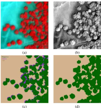
of Iran, which in UTM projection is located between, ULX: 347949.3, ULY: 2786168.1 and LRX: 348126.9 , LRY: 2785990.5 on April 06, 2006. The studying area is located within Govatr Bay in the delta of Bahookalat River which is a part of Gandoo Protected Area and Bahoo wetland and demonstrated as position 10 in Figure 2 [Zahed et al., 2010]. The satellite simultaneously captures panchromatic (Pan) and multispectral (MS) digital im-agery with spatial resolution of 0.6 and 2.4 m at nadir, respec-tively. Thus, the scale factorSbetween MS (Figure 3(a)) and Pan (Figure 3(b)) images is 4. The Pan sensor captures the surface re-flectance within a wavelength range of 450 to 900 nm, while the MS sensor provides four spectral bands; i.e. blue (450-520 nm), green (520-600 nm), red (630-690 nm), near-IR (760-890 nm). The selected area comprises 300 by 300 panchromatic pixels and their corresponding multispectral pixels. In this dataset, we tried to select a pure studying area with some individual mangrove tree crowns, in the non-dense mangrove forest. Therefore, we were able to extract the trees accurately and evaluate the results. The reference map (Figure 3(c)) was produced using visual interpre-tation of the panchromatic image and pan sharpening product.

Figure 2: Govatr Bay mangorves forest; adopted from (Zahed et al., 2010)

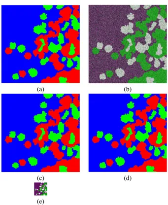
2) Simulated image: This dataset is a simulated image which was used to compare the accuracy of our improved adaptive MRF-SRM with that of [Li et al., 2013]. In order to generate this dataset, we employed the reference map of mangrove for-est dataset comprising 300 by 300 pixels, which contains real tree boundaries. Then, the trees are categorized into two differ-ent classes (class 1 and class2) to generate a reference map with complex class conditions (Figure 5(a)). The third class of this map is considered as soil. Then, we employed the (Mohn et al., 1987; Yu and Ekstrm, 2003) methodology as well as the proposed class mean values and class covariance matrix. The location of each distribution is presented as an ellipsoid in Figure 4. Then by utilizing the mean and covariance of the classes, a synthetic im-age with two bands and three classes was generated by sampling from the multivariate normal distribution. The generated image is degraded by scale factor 6 (Figure 5(b & c)) and utilized to apply adaptiveMRF-SPMand our improved adaptiveMRF-SRM.

To estimate the efficiency of the proposed spatially adaptive MRF-SPM [Li et al., 2012] and our improved adaptive MRF-SRM method, we applied both methods on the both datasets. Then the overall (OA), average (AA) and class-specific accuracies, as well as the kappa coefficient (k) are estimated. The resulting generated SRmaps for mangrove forest dataset are presented in Figure 3(d) and for the simulated image in Figures 5(c) and 5(d). Mangrove forest dataset contains two classes (mangrove and soils), thus the

(a) (b)

(c) (d)

Figure 3: (a) Three-band colour composite of QuickBird Image. (b) The panchromatic image of QuickBird Image. (c) Reference data of the mangrove forest dataset. (d) GeneratedSRmap using spatially adaptiveMRF-SPMmethod.

results of both spatially adaptiveMRF-SPM and our improved adaptiveMRF-SRMare the same.

In order to evaluate the performance of bothSRMmethods, we applied five state-of-the-art classification techniques, namely max-imum likelihood (ML), Mahalanobis distance (MaD), minimum distance (MiD), spectral angle mapper (SAM), and spectral cor-relation mapper (SCM) on the original simulated image and the fused image of MS and Pan for the mangrove forest dataset. All the classification methods were trained with similar training data sets (36 pixels per class) and their performance was evaluated by their corresponding reference maps. The results are reported in Table I, from which, it can be concluded that the improved adaptive MRF-SRM compared to the spatially adaptive MRF-SPM increased the overall accuracy by 5.1 percent. Although all the pixel based classification methods were applied on the original simulated image with scale factor 1 instead of scale fac-tor 6 which was utilized for both spatially adaptive MRF-SPM and improved adaptiveMRF-SRM methods, theOA,AA, andk of bothSRgenerated maps are higher thanSAM,SCMandMiD classified maps results (Table 1).

We evaluated the statistical significance of the difference between all the classification results in terms of accuracy by using the Mc-Nemars test with the 5% significance level for each pair of the classification maps [Aghighi et al., 2014]. According to the cal-culatedχ2 _{andzvalues, the null hypothesis (H}

0) of no signif-icant difference between map accuracies is rejected. Thus, the results of improved adaptiveMRF-SRM and spatially adaptive MRF-SPMare not the same as each other nor the other classified maps. This means that the use of the proposed improved adaptive MRF-SRMis beneficial to overcome the mixed pixel problem and it is suitable to produce a fine resolution ITC map or to extract the forest spatial patterns within coarse pixels.

state-Figure 4: Class expectation±2 standard deviation contours; in the case of spatial independency between pixels.

Table 1: Classification accuracy in percentage for each class of the simulated image, whereOA, AA, k, SA MRF-SPM, and IA MRF-SRMrepresent the overall accuracy, average accuracy, kappa coefficient, spatially adaptiveMRF-SPM, and improved adaptiveMRF-SRM.

SA MRF-SPM IA MRF-SRM ML SAM SCM MiD MaD

OA 89 94.1 96 78 78.5 85.4 95.5

AA 87.4 87.8 93.6 67.5 46.6 81.5 92.6

K 0.81 0.83 0.93 0.62 0.59 0.75 0.93

C 1 88.3 89.7 98.8 56.4 62.4 65.9 97.4 C 2 83.1 84.9 93.9 46.6 37.5 79.1 81.4 C 3 90.9 92.2 95.4 99.3 86.8 99.6 99.2

of-the-art approaches for ITC delineation. Therefore, we ap-plied different pan-sharpening methods, called subtractive res-olution merge, HPF resres-olution merge, Wavelet resres-olution merge, and Ehlers resolution merge on mangrove forest dataset pan-sharpened images. Then,ML,MaD,MiD,SAM, andSCMpixel based classification methods were employed to classify the gen-erated pan-sharpened images. In these experiments, the similar training data sets (36 pixels per class) were utilized to train the classification methods and their performance evaluated by the mangrove forest reference maps (Table 2).

From Table 2, it can be seen that the overall accuracy of the gen-erated mangrove forest using the spatially adaptiveMRF-SPM methods are higher than the overall accuracy of all classification methods using the pan-sharpened images, except for Subtractive resolution merge employing spectral angle mapper method. The calculatedχ2_{andzvalues for spatially adaptiveMRF-SPMand} each of the other classification methods indicate that the null hy-pothesis (H0) of no significant difference between map accura-cies are strongly rejected. Thus, both improved adaptive MRF-SRM method and spatially adaptive MRF-SPM are suitable to produce a fine resolution mangrove forest map or to extract the forest spatial patterns within coarse pixels. However, due to bet-ter performance of the improved adaptiveMRF-SRMthan spa-tially adaptiveMRF-SPMfor the simulated image with non-equal covariance matrices, it can be concluded that the proposed im-proved adaptiveMRF-SRMmethod could be more suitable than the spatially adaptiveMRF-SPMfor real images with non-equal covariance matrix for the classes (Table 1). Moreover, the ter-mination conditions of the improved adaptive MRF-SRM were satisfied three times faster when compared to spatially adaptive MRF-SPMfor simulated images.

(a) (b)

(c) (d)

(e)

Figure 5: (a) Reference map of simulated dataset. (b) Simulated image with 2 bands and scale factor 1. (c) Adaptive MRF-SPM result. (d) Improved adaptive MRF-SRM result. (e) The real proportional size of degraded simulated image with scale factor 6 (produced from Figure 5(b)) which is used to generate SR maps presented in Figures 5(c & d)) .

4. CONCLUSION

In this work, we have investigated the use of the proposed spa-tially adaptiveMRF-SRMto generate finer spatial resolution man-grove forest maps from a multispectral image with lower spatial resolution. This method is applied on QuickBird satellite images over the mangrove forest and its results are compared with 20 different classified maps produced by five different pixel based classification methods on four different pan-sharpened images. Experimental results have demonstrated that the accuracy of the generated mangrove forest maps are mostly better than the results of other techniques.

Table 2: the classification accuracy in percentage for each class of the the mangrove forest image, whereOA,AA,k, andSA MRF-SPMdenote the overall accuracy, average accuracy, kappa coef-ficient, and spatially adaptiveMRF-SPM.

SA MRF-SPM ML SAM SCM MiD MaD Subtractive resolution merge OA 92.7 87 93 89.3 90.9 86.9 AA 92.1 87.2 92.5 89.1 90.3 87.2 K 0.85 0.74 0.86 0.78 0.81 0.74 C 1 87.9 76.1 89.3 62.4 84.8 76 C 2 96.3 98.4 95.7 37.5 95.7 98.4

HPF resolution merge

OA 92.7 83.3 91.7 88.8 91.9 83.3 AA 92.1 85 91.1 0.78 91.3 85

K 0.85 0.67 0.83 88.6 0.83 0.67 C 1 87.9 70.6 87.1 79.3 87.7 70.5 C 2 96.3 99.4 95 97.8 94.9 99.5

Wavelet resolution merge

OA 92.7 79.5 81.2 80.3 81.2 79.4 AA 92.1 79.7 80.3 80 80.4 79.6 K 0.85 0.59 0.61 0.6 0.61 0.59 C 1 87.9 68.8 74.1 70.6 73.8 68.7 C 2 96.3 90.6 86.6 89.3 86.9 90.6

Ehlers resolution merge

OA 92.7 84.1 91.3 91.3 90.9 84 AA 92.1 85.5 90.7 90.7 90.2 85.5

K 0.85 0.69 0.82 0.82 0.8 0.69 C 1 87.9 71.4 89.9 86.9 85.7 71.4 C 2 96.3 99.6 94.5 91.5 94.8 99.6

REFERENCES

Aghighi, H., Trinder, J., Tarabalka, Y. and Lim, S., 2014. Dy-namic block-based parameter estimation for MRF classification of high-resolution images. Geoscience and Remote Sensing Let-ters, IEEE 11(10), pp. 1687–1691.

Ardila, J. P., Tolpekin, V. A., Bijker, W. and Stein, A., 2011. Markov-random-field-based super-resolution mapping for iden-tification of urban trees in VHR images. ISPRS Journal of Pho-togrammetry and Remote Sensing 66(6), pp. 762–775.

Atkinson, P., 1991. Optimal ground-based sampling for remote sensing investigations: estimating the regional meant. Interna-tional Journal of Remote Sensing 12(3), pp. 559–567.

Atkinson, P. M., 1997. Mapping sub-pixel boundaries from re-motely sensed images. Innovations in GIS 4, pp. 166–180.

Atkinson, P. M., Pardo-Iguzquiza, E. and Chica-Olmo, M., 2008. Downscaling cokriging for super-resolution mapping of continua in remotely sensed images. Geoscience and Remote Sensing, IEEE Transactions on 46(2), pp. 573–580.

Bagley, J. E., Desai, A. R., Harding, K. J., Snyder, P. K. and Foley, J. A., 2014. Drought and deforestation: Has land cover change influenced recent precipitation extremes in the Amazon. Journal of Climate 27(1), pp. 345–361.

Boucher, A. and Kyriakidis, P. C., 2006. Super-resolution land cover mapping with indicator geostatistics. Remote Sensing of Environment 104(3), pp. 264–282.

Boucher, A., Kyriakidis, P. C. and Cronkite-Ratcliff, C., 2008. Geostatistical solutions for super-resolution land cover mapping. Geoscience and Remote Sensing, IEEE Transactions on 46(1), pp. 272–283.

Bouman, C. A. and Shapiro, M., 1994. A multiscale random field model for bayesian image segmentation. Image Processing, IEEE Transactions on 3(2), pp. 162–177.

Clark, M. L., Roberts, D. A. and Clark, D. B., 2005. Hyperspec-tral discrimination of tropical rain forest tree species at leaf to crown scales. Remote Sensing of Environment 96(3), pp. 375– 398.

Erikson, M., 2003. Segmentation of individual tree crowns in colour aerial photographs using region growing supported by fuzzy rules. Canadian Journal of Forest Research 33(8), pp. 1557–1563.

Gong, P., Sheng, Y. and Biging, G., 2002. 3D model-based tree measurement from high-resolution aerial imagery. Photogram-metric Engineering & remote sensing 68(11), pp. 1203–1212.

Halounov, L., 2003. Textural classification of B& W aerial pho-tos for the forest classification. In: EARSeL conference.

Houghton, R. A., 2005. Tropical deforestation as a source of greenhouse gas emissions. Tropical deforestation and climate change p. 13.

Houghton, R., Skole, D., Nobre, C. A., Hackler, J., Lawrence, K. and Chomentowski, W. H., 2000. Annual fluxes of carbon from deforestation and regrowth in the Brazilian Amazon. Nature 403(6767), pp. 301–304.

Jepma C.J., C. J., 2014. Tropical deforestation: a socio-economic approach. Taylor & Francis.

Jing, L., Hu, B., Noland, T. and Li, J., 2012. An individual tree crown delineation method based on multi-scale segmentation of imagery. ISPRS Journal of Photogrammetry and Remote Sensing 70, pp. 88–98.

Kasetkasem, T., Arora, M. K. and Varshney, P. K., 2005. Super-resolution land cover mapping using a Markov random field based approach. Remote Sensing of Environment 96(34), pp. 302–314.

Koch, B., Heyder, U. and Weinacker, H., 2006. Detection of individual tree crowns in airborne lidar data. Photogrammetric Engineering & Remote Sensing 72(4), pp. 357–363.

Li, X., Du, Y. and Ling, F., 2012. Spatially adaptive smooth-ing parameter selection for Markov random field based sub-pixel mapping of remotely sensed images. International Journal of Re-mote Sensing 33(24), pp. 7886–7901.

Li, X., Du, Y. and Ling, F., 2013. Super-resolution mapping of forests with bitemporal different spatial resolution images based on the spatial-temporal Markov random field. Selected Topics in Applied Earth Observations and Remote Sensing, IEEE Journal of PP(99), pp. 1–11.

Liguo, W., Qunming, W. and Danfeng, L., 2011. Sub-pixel map-ping based on sub-pixel to sub-pixel spatial attraction model. In: Geoscience and Remote Sensing Symposium (IGARSS), 2011 IEEE International, pp. 593–596.

Ling, F., Li, X., Du, Y. and Xiao, F., 2013. Sub-pixel mapping of remotely sensed imagery with hybrid intra-and inter-pixel depen-dence. International Journal of Remote Sensing 34(1), pp. 341– 357.

Lu, D. and Weng, Q., 2007. A survey of image classifica-tion methods and techniques for improving classificaclassifica-tion perfor-mance. International Journal of Remote Sensing 28(5), pp. 823– 870.

Luciani, P. and Chen, D., 2011. The impact of image and class structure upon sub-pixel mapping accuracy using the pixel-swapping algorithm. Annals of GIS 17(1), pp. 31–42.

Makido, Y., Shortridge, A. and Messina, J. P., 2007. Assessing alternatives for modeling the spatial distribution of multiple land-cover classes at sub-pixel scales. Photogrammetric Engineering and remote sensing 73(8), pp. 935.

Mas, J.-F., Puig, H., Palacio, J. L. and Sosa-Lpez, A., 2004. Mod-elling deforestation using GIS and artificial neural networks. En-vironmental Modelling & Software 19(5), pp. 461–471.

Mertens, K. C., De Baets, B., Verbeke, L. P. and De Wulf, R. R., 2006. A sub-pixel mapping algorithm based on sub-pixel/pixel spatial attraction models. International Journal of Remote Sens-ing 27(15), pp. 3293–3310.

Mertens, K., Verbeke, L., Ducheyne, E. and De Wulf, R., 2003a. Using genetic algorithms in sub-pixel mapping. International Journal of Remote Sensing 24(21), pp. 4241–4247.

Mertens, K., Verbeke, L., Ducheyne, E. and De Wulf, R., 2003b. Using genetic algorithms in sub-pixel mapping. International Journal of Remote Sensing 24(21), pp. 4241–4247.

Powell, R. L., Roberts, D. A., Dennison, P. E. and Hess, L. L., 2007. Sub-pixel mapping of urban land cover using multiple endmember spectral mixture analysis: Manaus, Brazil. Remote Sensing of Environment 106(2), pp. 253–267.

Qunming, W., Wenzhong, S. and Liguo, W., 2014. Indicator cokriging-based subpixel land cover mapping with shifted im-ages. Selected Topics in Applied Earth Observations and Remote Sensing, IEEE Journal of 7(1), pp. 327–339.

Richards, J. and Jia, X., 2006. Remote sensing digital image analysis an introduction. Springer, Germany.

Shen, Z., Qi, J. and Wang, K., 2009. Modification of pixel-swapping algorithm with initialization fr om a sub-pixel/pixel spatial attraction model. Photogrammetric Engineering & Re-mote Sensing 75(5), pp. 557–567.

Solberg, A. H. S., Taxt, T. and Jain, A. K., 1996. A markov random field model for classification of multisource satellite im-agery. Geoscience and Remote Sensing, IEEE Transactions on 34(1), pp. 100–113.

Tatem, A. J., Lewis, H. G., Atkinson, P. M. and Nixon, M. S., 2001. Multiple-class land-cover mapping at the sub-pixel scale using a Hopfield neural network. International Journal of Applied Earth Observation and Geoinformation 3(2), pp. 184–190.

Tatem, A. J., Lewis, H. G., Atkinson, P. M. and Nixon, M. S., 2002. Super-resolution land cover pattern prediction using a Hop-field neural network. Remote Sensing of Environment 79(1), pp. 1–14.

Thornton, M., Atkinson, P. and Holland, D., 2006. Sub-pixel mapping of rural land cover objects from fine spatial resolution satellite sensor imagery using super-resolution pixel-swapping. International Journal of Remote Sensing 27(3), pp. 473–491.

Tolpekin, V. A. and Stein, A., 2009. Quantification of the effects of land-cover-class spectral separability on the accu-racy of Markov-random-field-based superresolution mapping. Geoscience and Remote Sensing, IEEE Transactions on 47(9), pp. 3283–3297.

Tolpekin, V. A., Ardila, J. P. and Bijker, W., 2010. Super-resolution mapping for extraction of urban tree crown objects from VHR satellite images. Small 3(1), pp. 1.

Verhoeye, J. and De Wulf, R., 2002. Land cover mapping at sub-pixel scales using linear optimization techniques. Remote Sensing of Environment 79(1), pp. 96–104.

Wang, Q., Wang, L. and Liu, D., 2012. Integration of spatial at-tractions between and within pixels for sub-pixel mapping. Sys-tems Engineering and Electronics, Journal of 23(2), pp. 293–303.

Warner, T. A., Lee, J. Y. and McGraw, J. B., 1998. Delineation and identification of individual trees in the eastern deciduous for-est. Automated interpretation of high spatial resolution digital imagery for forestry pp. 10–12.

Yong, X. and Bo, H., 2014. A spatio & temporal pixel-swapping algorithm for subpixel land cover mapping. Geoscience and Re-mote Sensing Letters, IEEE 11(2), pp. 474–478.

Zahed, M. A., Ruhani, F. and Mohajeri, S., 2010. An overview of iranian mangrove ecosystem, northern part of the Persian gulf and Oman sea. Electronic Journal of Environmental, Agricultural and Food Chemistry 9(2), pp. 411–417.

Zhang, J., 2010. Multi-source remote sensing data fusion: status and trends. International Journal of Image and Data Fusion 1(1), pp. 5–24.

Zhang, L., Wu, K., Zhong, Y. and Li, P., 2008. A new sub-pixel mapping algorithm based on a BP neural network with an obser-vation model. Neurocomputing 71(10), pp. 2046–2054.