Development and Implementation of a Low-Cost
LBL Navigation System for an AUV
Aníbal Matos, Nuno Cruz, Alfredo Martins and Fernando Lobo Pereira
Faculdade de Engenharia da Universidade do Porto and
Instituto de Sistemas e Robótica
R. dos Bragas, 4050-123 Porto
Portugal
{anibal,nacruz,aom,flp}@fe.up.pt
Abstract — A reliable navigation system is a key factor
for the success of an operational mission with an AUV in a real scenario. In this paper, we address the main issues involved in the implementation of a long baseline (LBL) navigation system for a REMUS AUV. This system replaces both the original hardware and software of the vehicle with a simpler, faster, less expensive and more precise system, based on a Kalman filter. We also discuss the influence of transponder location in the overall performance of the LBL navigation, and present results obtained with this new system in operational missions.
I. INTRODUCTION
The autonomous operation of an AUV requires an on-board navigation system to compute, in real-time, the position of the vehicle. There are many different systems to determine the position of an AUV [1]. For low cost AUVs an acoustic position system complemented with velocity measurements seems to be the most common solution [1,2,3].
In this paper we describe a new navigation system developed for Isurus, a REMUS class AUV [4]. This is a torpedo shaped vehicle with a diameter of 20 cm and about 1.5 meters long. The propulsion is provided by a rear placed propeller and the vehicle has horizontal and vertical control surfaces to change its position both in the vertical and the horizontal planes. The vehicle is equipped with a set of sensors for navigation and control: a pressure cell to measure the vehicle depth, a digital magnetic compass to determine its heading, two tilt sensors that measure the vehicle roll and pitch angles, a shaft encoder to measure the propeller rotation speed and sensors to determine the angular position of the control surfaces. The vehicle has also an omni-directional acoustic transducer. This transducer is capable of transmitting and receiving acoustic signals in the medium frequency range (20kHz to 30kHz).
The new navigation system replaces the original Remus navigation system. The original system could be used to navigate either in LBL or USBL mode and used a DSP to process the acoustic signals received by the vehicle. The new system operates only in LBL mode and the DSP based signal detection was replaced by analog filters tuned to the
frequencies of the signals emitted by the transponders. An algorithm that fuses range measurements with dead-reckoning information was also implemented in the on-board computer.
This algorithm was implement in the new structure of the on-board software that has been developed for Isurus [5,6], using a real time operating system.
This paper is organized as follows. In section 2, we describe the overall structure of the navigation system. In section 3, we discuss the sensitivity of the positioning algorithm as a function of the location of the vehicle with respect to the transponders and of the location of the transponders themselves. In sections 4 and 5, we present the two parts of the developed system: the acoustic signal detection hardware, and the algorithm that merges the dead reckoning information and the range measurements to produce an estimate of the vehicle position. In section 6, we present some results achieved with this system in a real mission performed by the vehicle.
II. SYSTEM DESCRIPTION
The main function of the developed navigation system is to determine the position of the vehicle in the horizontal plane, as the vertical coordinate of the vehicle is given directly from the pressure cell. To perform such a task, the navigation system uses range measurements to a set of acoustic transponders deployed in the area of operation and information of the vehicle velocity relative to the water. To obtain a range measurement, the vehicle has to transmit an interrogation signal to a given transponder, detect the reply from the transponder and measure the round trip travel time of the acoustic signal. The vehicle velocity is obtained by measuring the propeller rotation speed and the vehicle heading, pitch and roll.
Velocity measurements are fused with range measurements by a Kalman filter based algorithm, taking advantage of the characteristics of each type of data. On one hand, the vehicle velocity data is available at a high rate, but its integration leads to a drift in the estimated position. On the other, range measurements, available at a lower rate, can be noisy but do not drift over time. The algorithm updates the estimate of the vehicle position at the same rate the velocity is measured, and
corrects it whenever a new range measurement is received, giving the best estimated vehicle position in real-time.
The navigation system is also responsible for the real time definition of the sequence of interrogation of the transponders. This is made in such a way that it tries to maximize the quality improvement of the estimated position.
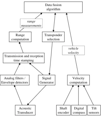
Figure 1 shows the modules that compose the navigation system and the information flow among them.
Acoustic Transducer Velocity computation Shaft encoder Digital compass Tilt sensors Signal Generator Analog filters / Envelope detectors
Transmission and reception time stamping Range computation Transponder selection Data fusion algorithm range measurements vehicle velocity
Fig. 1 – Navigation system modules.
III. LBL POSITIONING ANALYSIS
On a LBL positioning system, the absolute position of a vehicle can be obtained in a two step procedure. First, the position of the vehicle in a coordinate frame associated to the transponders is computed, based on the range to the transponders and on the relative location of the transponders. Then, a change of coordinates is made to obtain the position of the vehicle in an Earth fixed frame.
As the position of the vehicle is obtained as a function of the ranges to the transponders and of the location of the transponders themselves, the accuracy of the LBL positioning depends on the accuracy of the range measurements and on the accuracy of the positioning of the transponders (both relative to each other and absolute).
As the expressions that relate the ranges to the transponders with the LBL positioning solution are nonlinear, the sensitivity of the positioning solution to errors in range measurements and to the positioning of the transponders varies from place to place. Therefore, to get the best accuracy with the LBL positioning, the vehicle should operate in an area where that sensitivity has low values. Or, put in another way, given an area where the vehicle is intended to operate, the locations of the transponders should be chosen in such a way that this
sensitivity has low values in that area.
These sensitivity problems becomes particularly relevant when using only two transponders to determine the vehicle position in the horizontal plane. It is obvious that, in such case, there are two possible solutions for the positioning problem. Nevertheless, this ambiguity can be avoided if the vehicle does not cross the baseline (that is, the line connecting the transponders), and its initial position with respect to that line is known. -200 0 200 400 600 0 100 200 300 400 500 600 700 800 east (m ) north (m) 1.2 1.4 1.6 1.8 2 2 1.8 1.6 1.4 1.2 Tx1 Tx2
Fig. 2 – Sensitivity of positioning to range errors.
-200 0 200 400 600 0 100 200 300 400 500 600 700 800 east (m) north (m) 2 1.2 1.2 1.4 1.6 1.8 2 Tx2 Tx1
Fig. 3 – Sensitivity of positioning to errors in the distance between transponders.
Figures 2 and 3 present the level contours of the positioning sensitivity to errors in range and to the distance between the transponders, respectively, for the LBL positioning using two transponders (Tx1 and Tx2).
baseline and outside the region between the transponders. In the first case the sensitivity also takes higher values far form the transponders. Therefore, as a practical rule we define the best area for the operation can be defined as a box as show in figure 4. The minimum distance to the baseline is one fourth of the distance between the transponders and the maximum distance is equal to the distance between the transponders.
-50 0 50 100 150 200 250 300 350 400 450 -50 0 50 100 150 200 250 300 350 400 450 500 east (m) north (m) Tx1 Tx2
Fig. 4 – Desirable operation area.
IV. RANGE MEASUREMENTS
One important part of the developed navigation system is the subsystem that measures the ranges to the transponders. To obtain a range measurement to one transponder, the vehicle has to interrogate it, detect its reply and measure the round trip travel time of the acoustic wave.
The signals used to interrogate the transponders are pure tones of a few milliseconds duration. As each transponder listens to a different frequency, the frequency of the interrogation signal automatically selects a single transponder.
The replies from the transponders are also pure tone signals and each transponder uses a different frequency, being all of them different from the interrogation frequencies, too.
To detect replies from the transponders, the navigation system uses analog filters with high Q factors. Each one of these filters is tuned to the reply frequency of one of the transponders. The output of each of these filters is connected to an envelope and level detector circuit. The actual detection of a reply from a transponder is made by comparing the output level of the respective envelope detector with an adjustable threshold. These thresholds can be set to reflect the ambient noise of the operation area and the expected ranges to the transponders.
An embedded micro-controller is used to measure the travel time of the acoustic signals. To perform such a task, this micro-controller monitors the transmission of the interrogation signals and the detection circuits. The micro-controller keeps an internal clock (with a resolution of 100 µs), and, whenever a new interrogation signal is transmitted or a reply signal is detected time-stamps the event and sends an appropriate message to the on-board CPU. The on-board software is then responsible to match the received replies with pending
interrogations and compute the ranges to the transponders. Since the electronic filters do not use any digital signal processing, they are prone to be fouled by multi-path echoes. Nonetheless, the robustness of the Kalman filter based algorithm ensures that spurious range measurements are easily detected and rejected. On the other hand, the absence of any digital signal processing makes the range measurements available to the navigation algorithm as soon as the replies from the transponders are received. This fact is quite significant for two main reasons:
• as the vehicle is moving, the lower the delay between the reception of the transponder reply and the processing of the range measurement by the navigation algorithm, the better is the navigation accuracy; • it permits to have higher interrogation rates that lead to
better a navigation accuracy.
V. NAVIGATION ALGORITHM
The algorithm used to estimate the position of the vehicle in the horizontal plane is based on a Kalman filter [7]. This algorithm uses a very simple model of the vehicle motion to predict its evolution based on the measurements of the propeller speed and the vehicle heading, pitch and roll, and corrects the estimate of the vehicle position as soon as a new range measurement is available. In this way, the algorithm makes the best use of the different characteristics of the available data.
Besides the estimation of the vehicle position, the algorithm also estimates the water current (in the horizontal plane) and can even be used to estimate several parameters that relate the rotation speed of the propeller and the heading, pitch and roll of the vehicle to the horizontal velocity of the vehicle with respect to the water (in steady state).
For the sake of clarity we will present the simplest version of the navigation algorithm, that is, the one that just estimates the position of the vehicle and the speed of the water.
A. Filter Data
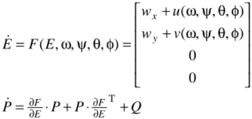
The filter state E = [x y wx wy] is composed by estimates of the north and east coordinates of the vehicle and of the north and east components of the water speed, respectively.
Besides the state E, the filter also keeps a matrix P, the error covariance matrix, that measures the covariance of the estimation error.
The 2×2 sub-matrix of the matrix P, denoted Pxy,
corresponding to the x and y components of the filter state E, can be used to measure the quality of the current estimate of the vehicle position. The matrix Pxy defines an ellipse in the
plane that characterises the error of the position estimate. This ellipse in defined by 3 parameters: the lengths of its two principal axes and the orientation of its major axis.
B. Dead-reckoning estimation
Between the reception of two consecutive range measurements, the evolution of E and P is ruled by the
following differential equations: φ θ ψ ω + φ θ ψ ω + = φ θ ψ ω = 0 0 ) , , , ( ) , , , ( ) , , , , ( w v u w E F E y x & Q P P P&=∂∂EF⋅ + ⋅∂∂EFT+
In these equations, ω, ψ, θ, and φ, are respectively, the propeller rotation speed, and the heading, pitch and roll of the vehicle; u(⋅) and v(⋅) give the north and east components of the velocity of the vehicle (w.r.t. the water) as a function of ω, ψ, θ, and φ, in steady state [8]; Q is a, possibly time-varying, symmetric semi-positive definite matrix representing the rate of increase of the estimation error due to the fact that the vehicle motion is not exactly modeled by the above equation. This matrix is used to tune the filter behavior, shaping its frequency response.
The values of E and P are update at the same rate of the main control loop of the vehicle: 10 Hz.
C. Range corrections
Whenever a new range measurement is received and is validated, the state E and the covariance matrix P are corrected according to the expressions:
) (r r* K E E+ = −+ ⋅ − − − + =P −K⋅H⋅P P
where E− and P− are the values of the E and P before the correction and E+ P+ are their values after the correction; r is the measured range and r* is the expected range, that is
2 2
2
* (x x) (y y) (z z)
r = −− + −− + −
where z is the depth of the vehicle and (x,y,z) are the coordinates of the transponder. The matrices H and K are given by: = = − − = ∂ ∂ − − − 0 0 | * * * r y y r x x E E E r H 1 T − −⋅ ⋅ =P H S K where q H P H S= ⋅ −⋅ T+
and q represents the variance of the error in each range measurement.
A range measurement is considered valid if γ ≤ − *||2−1
||r r S
where γ is a parameter chosen to prevent spurious range measurements from being considered in the estimation of the vehicle position.
D. Transponder selection
The navigation algorithm is also responsible for the definition of the sequence of interrogation of the transponders. If, for the two transponders case, this selection is quite obvious (the transponders should be interrogated in an alternate way), it is important to establish some criteria to define in real time the sequence of interrogations when there are several transponders. There is an obvious way to select, at each time, the next transponder to interrogate: it should be the transponder that, after the range correction, leads to a better estimate of the vehicle position [9].
One way to measure the quality of the position estimate corrected by a range measurement to transponder k, is to compute the following value:
2 ) ( ) ( 1 ||( , )|| 2 2 xy k k y y k k P x x k x x y y m = ⋅ − − − + −
where (x, y) is the estimated vehicle position in the horizontal plane; and (xk, yk) is the position of transponder k in the
horizontal plane. At each moment, the transponder to be interrogated should be selected as the one that maximizes the figure of merit mk. The idea behind this criteria is to select the
transponder that is in the direction along which the uncertainty of the position estimation is greater.
Besides the decision of which transponder to interrogate, it is also necessary to define when the transponder should be interrogated. The algorithm implemented interrogates one transponder immediately after the reception of the reply from the previous interrogated transponder, or after a given timeout, if there is no reply from pending interrogation. Although this technique does not lead to the maximum possible interrogation rate, it reduces the probability of receiving long multi-path replies from previous interrogations of the same transponder.
The interrogation of one transponder immediately after the reception of the previous reply was implemented to allow for tracking of the vehicle with an external device, as is described in [10].
VI. EXPERIMENTAL DATA
The navigation system described in this paper has been successfully tested in real application scenarios. It is currently being used in operational missions with Isurus, performed in the estuary of Minho river on the northern border of Portugal [10].
Figure 5 shows the trajectory of the vehicle in an operational mission in that scenario. In this mission the vehicle was collecting CTD and bathymetry data, and its position was being estimated by the navigation algorithm presented here. The vehicle traveled at an average speed of about 1.2 m/s, for more than 2000 meters.
As shown in the figure, the navigation system was using only two transponders, and although there were a period of time when the vehicle was very close to the baseline (less than 30m, which is about 1/20th of the baseline length) the performance of the navigation algorithm was quite good. It is also possible to notice that the estimated trajectory is quite
smooth, showing the good behavior of the navigation algorithm. 0 100 200 300 400 500 -400 -300 -200 -100 0 100 Start Finish Tx1 Tx2 east (m) north (m)
Fig. 5 – Vehicle trajectory during an operational mission.
0 200 400 600 800 1000 1200 1400 1600 1800 2000 0 1 2 3 4 5 6 time (s) estimation error de v iation (m)
Fig. 6 – Length of the axes of the estimation error ellipse.
Figure 6 shows the lengths of the two principal axes of the ellipse that characterises the error of the estimated position. As can be easily seen in the figure, when the vehicle was travelling near the baseline, the lengths of major and minor axes of the ellipse were quite different, showing that the estimated position was much more accurate in one direction (parallel to the baseline) than in the other (normal to the baseline). This is a direct consequence of the sensitivity problems already discussed. In the last part of the mission, the vehicle was travelling in an area where the sensitivity of the LBL positioning has low values, and there, the two axes of the ellipse were almost of the same length.
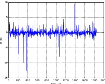
Figure 7 shows the differences between range measurements and their estimated values. These differences can be used to measure the performance of the navigation algorithm. As the figure shows, these differences, except for a
few cases, assume very low values, showing the good performance of the navigation system.
0 200 400 600 800 1000 1200 1400 1600 1800 2000 -15 -10 -5 0 5 10 time (s) dr (m)
Fig. 7 – Differences between measured and estimated ranges.
VII. CONCLUSIONS AND CURRENT WORK The results already obtained with real applications of this navigation system show a significant improvement of performance over the REMUS original navigation system.
Even in the estuary of Minho river, a very shallow water environment, the new navigation system proved to be robust to multi-path echoes. This robustness is accomplished by the validation of the range measurement, as the analog acoustic detection system is easily fouled by such echoes.
The analysis of the sensitivity of the LBL positioning contributed to the good performance of the navigation, as the locations of the transponders were chosen according to the criteria presented here, whenever possible.
We are now testing more elaborate filters with data acquired in real missions. These filters take into account a model of the hydrodynamic behavior of the vehicle. The tests, yet not completely conclusive, show that theses filters require much more computational power to operate in real time, and that the quality of the navigation does not increase that much.
Another issue under research is the use of post mission smoothing algorithms to improve the accuracy of the space stamping of the CTD and bathymetry data collected by the vehicle [10].
REFERENCES
[1] J. Leonard, A. Bennett, C. Smith, H. Feder. Autonomous Underwater Vehicle Navigation. MIT Marine Robotics Laboratory Technical Memorandum 98-1.
[2] J. Vaganay, J. Leonard, J. Bellingham. Outlier Rejection for Autonomous Acoustic Navigation. In Proceedings of the IEEE International Conference on Robotics and Automation, Minneapolis, MN, April, 1996.
[3] J. Bellingham, T. Consi, U. Tedrow, D. Di Massa. Hyperbolic Acoustic Navigation for Underwater
Vehicles: Implementation and Demonstration. In Proceedings of the AUV’92 Conference, 1992.
[4] C. Alt, B. Allen, T. Austin, R. Stokey. Remote Environmental Measuring Units. In Proceedings of the Autonomous Underwater Vehicle's 94 Conference, Cambridge, MA, USA, July 1994, pp. 13-19.
[5] J. Silva, A. Martins, F. Lobo Pereira. A Reconfigurable Mission Control System for Underwater Vehicles. To apper in Proceedings of the MTS/IEEE Oceans’99 Conference, Seatle, WA, USA, September, 1999.
[6] J. Sousa, N. Cruz, A. Matos, F. L. Pereira. Multiple AUVs for Coastal Oceanography. In Proceedings of the MTS/IEEE Oceans’97 Conference, Halifax, Canada, October, 1997.
[7] A. Gelb. Applied Optimal Estimation, MIT Press, 1989. [8] A. Martins. Isurus AUV Modeling, LSTS Internal Report
98-1, FEUP-DEEC, 1998 (in portuguese).
[9] J. Leonard, H. Durrant-Whyte. Directed Sonar Sensing for Mobile Robot Navigation, Kluwer Academic Publishers, 1992.
[10] N. Cruz, A. Matos, A. Martins, J. Silva, D. Santos, D. Boutov, D. Ferreira, F. Lobo Pereira. Estuarine Environment Studies with Isurus, a REMUS class AUV. To apper in Proceedings of the MTS/IEEE Oceans’99 Conference, Seatle, WA, USA, September, 1999.