ABSTRACT: In this paper, the dynamics of the relative motion problem in a perturbed orbital environment are exploited based on Gauss’ variational equations. The relative coordinate frame (Hill frame) is studied to describe the relative motion. A linear high idelity model is developed to describe the relative motion. This model takes into account primary gravitational and atmospheric drag perturbations. In addition, this model is used in the design of a control, guidance, and navigation system of a chaser vehicle to approach towards and to depart from a target vehicle in proximity operations. Relative navigation uses an extended Kalman ilter based on this relative model to estimate the relative position and velocity of the chaser vehicle with respect to the target vehicle and the chaser attitude and gyros biases. This ilter uses the range and angle measurements of the target relative to the chaser from a simulated Light Detection and Ranging (LIDAR) system, along with the star tracker and gyro measurements of the chaser. The corresponding measurement models, process noise matrix and other ilter parameters are provided. Numerical simulations are performed to assess the precision of this model with respect to the full nonlinear model.The analyses include the navigations errors, trajectory dispersions, and attitude dispersions.
KEYWORDS: Satellite relative motion, Orbital rendezvous.
Relative Motion Guidance, Navigation
and Control for Autonomous Orbital
Rendezvous
Mohamed Okasha1,2, Brett Newman2
INTRODUCTION
Although signiicant progress and technical development have been achieved with regards to orbital rendezvous such as International Space Station supply and repair and automated inspection, servicing, and assembly of space systems, there are limitations with the traditional methods that struggle to meet the new demands for orbital rendezvous. Presently, in order to perform such close proximity operations, mission controllers generally require signiicant cooperation between vehicles and utilize man-in-the-loop to ensure successful maneuvering of both spacecrat. he interest in autonomous rendezvous and proximity operations has increased with the recent demonstration of XSS-11, Demonstration of Autonomous Rendezvous Technology (DART), and Orbital Express. Autonomous rendezvous and proximity operations have also been demonstrated by Japanese EST-VII, and the Russian Progress vehicles. In addition future missions to the ISS will require autonomous rendezvous and proximity operations (Fehse, 2003; Woinden and Geller, 2007).
Many relative motion modeling and control strategies have been designed using the linearized Clohessy-Wiltshire (CW) equations to describe the relative motion between satellites. he CW equations are valid if two conditions are satisied:
• he distance between the chaser and the target is small compared tothe distance between the target and the center of the attracting planet; and
• he target orbit is near circular (Clohessy and Wiltshire, 1960).
he CW equations do not include any disturbance forces, for example, gravitational perturbations and environmental forces
1.International Islamic University Malaysia – Kuala Lumpur – Malaysia 2.Old Dominion University – Norfolk/VA – United States
Author for correspondence: Mohamed Okasha – Assistant Professor – Department of Mechanical Engineering – Faculty of Engineering–International Islamic University Malaysia
| Jalan Gombak | P.O. Box 10 50728 Kuala Lumpur – Malaysia | Email: [email protected] or Ph.D. Alumni from Old Dominion University | Email: [email protected]
(solar radiation pressure and atmospheric drag). Alternative linear equations that have been used in the literature to model the relative motion are the Tschauner-Hempel (TH) equations (Tschauner and Hempel, 1965).hese expressions generalize the CW equations and are similar to them in their derivation and types of applications. Tschauner and Hempel derived theses equations from the viewpoint of rendezvous of a spacecrat with an object in an elliptical orbit. They found complete solutions for elliptical orbits in terms of the eccentric anomaly. his advancement was followed by additional papers which present the complete analytical solution explicit in time, expanding the state transition matrix in terms of eccentricity (Yamanaka and Ankersen, 2002; Carter, 1998; Melton, 2000; Broucke, 2003; Inalhan et al., 2002; Sengupta and Vadali, 2007; Cho and Park, 2009). his form of solution is used to analyze the relative motion between the chaser and the target vehicles in the relative frame of motion more eiciently and rapidly than solving the exact nonlinear diferential equations in the inertial coordinate system. he TH equations do not take into account any perturbation forces. hese perturbations have a signiicant efect on the satellite relative motion.
Due to the previous limitations of the CW and TH models, this paper proposes an innovative linear model which includes both the perturbation that relects the Earth’s oblateness efect and atmospheric drag perturbation in the Cartesian coordinates orbital frame with little complication. Especially in low Earth orbits (LEOs), these perturbations have a deep inluence on the relative dynamics, and their inclusion in the linear model can sensibly increase the performance of the linear ilters, allowing greater insight of satellite relative motion, and providing an opportunity to investigate alternative feedback control strategies for the proximity operations.
Unlike the relative translation motion control, the relative rotational control is a traditional feedback control system. During the mission scenarios, the chaser vehicle may need to track the target vehicle to achieve proper docking maneuvers and or visual inspection tasks. he paper uses an extended Kalman ilter formulation to estimate the relative motion and chaser attitude using range and angle measurements from a LIDAR system coupled with gyro and star tracker measurements of the chaser (Woinder and Geller, 2007; Jenkins and Geller, 2007; Junkins et al., 2005; Woinden, 2004). he Kalman ilter basically consists of two main stages. he irst stage is the propagation stage, where the states are propagated numerically and it is based on the proposed linear model. he second stage comes
when the measurements from the sensors are available and it is used to update the states of the irst stage. he corresponding measurement models, process noise matrix, and other ilter parameters are provided. Momentum wheels are assumed for attitude control and thrusters are assumed for translation control. he efects of the navigation ilter, pointing algorithms, and control algorithms are included in the analysis.
he objective of this paper is as follows:
• To develop linearized high idelity models for relative motion in a perturbed orbit;
• To design a navigation ilter that can determine the relative position and velocity between target and chaser vehicles as well as orientations and angular rates of the chaserthat support closed-loop proximity attitude control operations and maneuvers; and
• To design a control system for the chaser vehicle to either approach or depart fromthe target vehicle in proximity operations in a general perturbed orbit for coupled translation and rotation relative motion.
he analysis in the current paper is summarized as follows. First, we present the relative dynamics equation of motion for the chaser with respect to the target in a general perturbed orbit, along with attitude dynamics models.Next, a linear high idelity relative motion model is developed to describe relative motion in proximity operations based on Gauss’ variational method. hen, the relative navigation and an extended Kalman ilter are presented for the relative motion and attitude estimations, along with the relative translational and rotational controller. In the simulation section, the accuracy and performanceof the relative navigation and controller, based on the high idelity model, are illustrated through diferent numerical examples and comparisons are made with the truth nonlinear model. Finally, conclusion of the work is presented and suggestions are made for future work.
RELATIVE MOTION MODELS
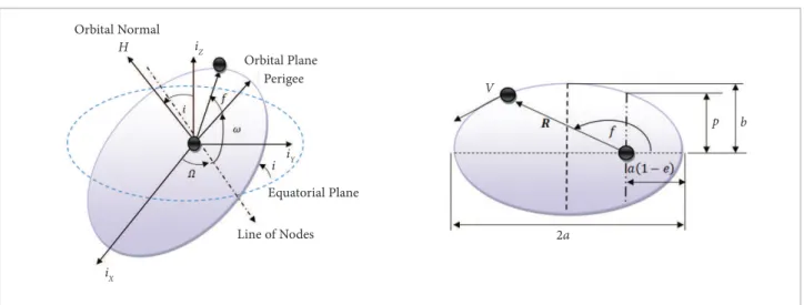
(LVLH) frame,which is attached to the target spacecrat , as shown in Fig.1. h is frame has basis {iX, iY, iZ,} with iX lying along the radius vector form the Earth’s center to the spacecrat , iZ coinciding with the normal to the plane dei ned by the position and velocity vectors of the spacecrat , and iY = iZ x iX. h e LVLH frame rotates with angular velocityvector ω, and its current orientation with respect to the ECI frame is given by the 3-1-3 direction cosine matrix, comprising right ascension of ascending node Ω, inclination i, perigee argument ω plus true anomaly f, respectively (Fig.2). h e angular velocity can also be expressed in terms of orbital elements and their rates.
Let the position of the chaser vehicle in the target’s LVLH frame be denoted by ρ=xix+yiy+ziz, where x, y and z denote the components of the position vector along the radial, transverse,
and out-of-plane directions, respectively. ρis determined from ρ=Rc-Rt, where Rc and Rt are the chaser and target absolute position vectors. h en, the most general equations modeling relative motion are given by the following:
(1)
where [fc]LVLH and [f
t]LVLH are the external accelerations acting
on the chaser and the target, respectively in the LVLH frame of the target vehicle. In Eq. (1), (..) and (.) denote the i rst and second derivatives with respect to time.
It is assumed, in this paper, that the externalaccelerations arise due to two basic groups of accelerations, dei ned by the following equation:
f = fg + fa + fc + fw (2)
h e i rst group of accelerationsis due to gravitational ef ects, fg, atmospheric drag, fa, and control, fc. Since Earth isn’t perfectly spherical, more accurate gravity models exist, taking into account Earth’s irregular shape. One irregularity that has a signii cant inl uence on space missions is the Earth’s bulge at the equator. h is phenomenon is captured in the J2 gravity model (Vallado, 2001; Schaub and Junkins, 2003). h e second group of accelerations, fw, is considered to be small accelerations, due to the gravity i elds of other planets, solar pressure, or venting, which also perturbs the spacecrat ’s motion. h ese small accelerationsare grouped together and modeled as zero mean normally distributed random variables (Woi nden and Geller, 2007).
Relative Orbit
Target
Chaser
Rc Rt
iY iY
iZ
iZ
iX
iX
ρ
Figure 1. Relative Motion Coordinates.
Figure 2. Orbital Elements.
Orbital Plane Orbital Normal
Perigee
Equatorial Plane
Line of Nodes
iX
iZ
iY i H
2a
In the literature, the most popular methods to model the spacecraft’s orbit are known as Cowell’s method and Gauss’s method (Vallado, 2001; Schaub and Junkins, 2003). The Cowell’s method is basically defined by specifying the position (R) and velocity (V) vectors of the spacecrat in the inertial coordinate frame, while Gauss’ method is dei ned by an equivalent set of elements called orbital elements (a,e,i,Ω,ω,f) which correspond to the semi-major axis, eccentricity, inclination, right ascension of the ascending node, argument of periapsis, and true anomaly, respectively, as shown in Fig. 2.
Table 1 summarizes the dynamic equations that are used in order to describe all of these methods. In this table, [.]I and [.]LVLH denote that the forces are dei ned in inertial and LVLH coordinate frames, respectively; ax , ay and az are the components of disturbance accelerations acting on the target in the LVLH reference coordinate frame; s(∙)=sin(∙) and c(∙)=cos(∙); and R are the Earth gravitational constant and the radius of the Earth; the terms R and V refer to the magnitude of the position and velocity vectors, respectively; the quantity H denotes the magnitude of the specii c angular momentum vector dei ned by H=R×V; X, Y and Z are the components of the spacecrat position vector; CD
Table 1. Orbit Model Methods Summary.
Method Dynamic equations
Cowell’s
is the atmospheric drag coei cient; A denotes the cross sectional area; m is the spacecrat mass; and i nally, ρ is the atmospheric density. Exponential atmospheric behavior is used to model Earth’s atmospheric density. h is model and its corresponding parameters are dei ned inVallado (2001).
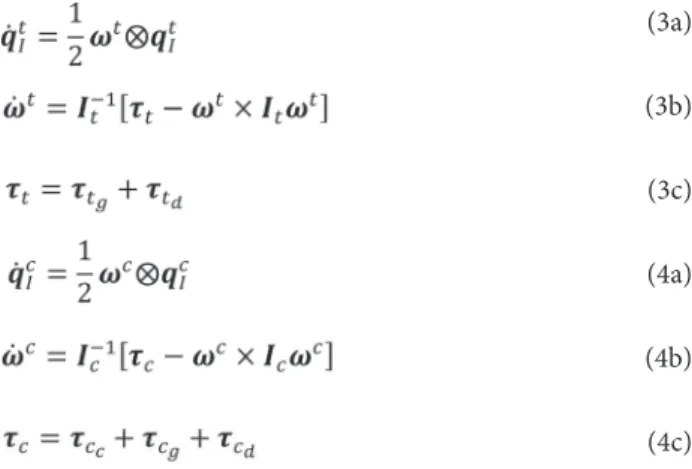
In order to use the generalized relative dynamic model dei ned by Eq. (1), the angular velocity vector, ω, and the angular acceleration vector, ώ, ot he LVLH frame with respect to the ECI frame, needs to be determined. Table 2 summarizes the equations that can be used to compute these vectors. h ese equations are derived based on using either Cowell’s method (position and velocity vectors) or Gauss’s method (orbital elements). In this table, the matrix TILVLH denotes the direction cosine matrix of the LVLH coordinate frame with respect to the ECI coordinate frame. h e Euler’s equation of motion is used to describe the attitude dynamics for both target and chaser vehicles, and a quaternion formulation is used for attitude kinematics. h e dynamics for both vehicles are given below as (Woi nden and Geller, 2007):
(3a)
(3b)
(3c)
(4a)
(4b)
(4c)
where is the quaternion multiplication operator dei ned by Lear (1985).
(5)
Dynamic equations
Given Inertial Position and Velocity
Given Orbital Elements
and the i vehicle gravity gradient torque is dei ned by
(6)
In Eqs. 3 and 4, the target states include the quaternion, qIt, that dei nes the orientation of the target with respect to the
inertial frame, and the target’s angular rate, ωt. Similarly the chaser
states are qIcand I
c. andare the target and chaser inertia matrices,
respectively. h e gravity gradient torque, τ(ig), for both vehicles (τ(cg) for the chaser and τ(tg) for the target) is derived from the Earth’spoint mass gravity models. h e random disturbances, τ(td) and, τ(tg) are included in the models to account for disturbance torques acting on each vehicle such as drag, solar radiation and other unmodeled disturbances. h ese unmodeled disturbances are represented as uncorrelated white noise, with mean and variance dei ned by a trial and error technique outlined by Lear (1985). h e control input, τ(cc), is the torque executed by the actuators (momentum wheels) on the chaser spacecrat .
It is assumed that the available sensors are the LIDAR for tracking the target and an assembly of a star tracker and gyros for attitude determination. h e parameter states for these sensors are modeled as i rst-order Markov processes with large time constants, causing them to behave like biases. h e parameter states include the gyros bias bωc, star camera misalignments Є
ss,
and LIDAR misalignments Єll. h e dynamics model associated
with these states is given by:
(7a)
(7b)
(7c)
where, wbω, ws and wl are white noise terms, driving the i
rst-order Markov processes and τbω, τs and τl are the corresponding
time constants.
The actuator models used in the simulation include momentum wheels for orientation control and thrusters for translational control. h e mathematical model for the actual control torque, generated by the wheels, and the impulsive thrust, by the thrusters, are:
(8)
(9)
h e generated torque and impulsive include errors such as noises νc, biases bc, scale factor biases fc, and misalignments Єc.
h ese errors can be modeled also as white noises.
h e simulation contains gyros, star tracker, and LIDAR sensor models. h e models for these measurements are given by:
Gyro Model:
(10)
Star Tracker Model:
(11)
LIDAR Model:
(12)
where:
(13)
h e gyro models include bias bωc, scale factor bias f ωc, and
angular random walk noise νωc. h e starcamera model accounts
for the uncertainty in the alignment of the star camera frame Єss with respect to the chaser frame and sensor noise ν
ss. h e
qcs refers to the i xed orientation of the star camera coordinate
frame with respect to the chaser body coordinate frame. h e LIDAR model includes angle measurements (azimuth, α, and elevation, β) noises vα, vβ and range (ρ) noise, vρ. h e transformation matrix denoted by Tab is the transformation
matrix used to transform any vector from coordinate b to coordinate a. h e term ilosl is the line of sight vector in the
LIDAR coordinate frame (Fig. 3). h e transformations TlῙ,
TῙS, TŜS, TŜI, and TITare a series of transformation matrices to
transform the line of sight vector from target LVLH coordinate frame to the LIDAR coordinate frame. h ese transformations include errors from sensor misalignments, noises, and attitude determination errors.
The small angle rotations can be written in terms of quaternions as
or attitude matrices as
(15)
where θ=θu is a small rotation vector, and θ× operating on
vector ω is a cross product matrix dei ned by the ordinary cross product θ× ω = ω × θ.
LINEAR HIGH FIDELITY RELATIVE
MODEL
In this section, a linear time varying high i delity model is obtained to describe the relative motion dynamics. h is model is derived based on two main assumptions. h e i rst assumption is that the relative distant between the chaser and the target vehicles is much less than the target orbital radius. h e second one assumes that the main disturbance accelerations, that af ect both vehicles are the gravitational acceleration and the atmospheric drag acceleration. Based on these assumptions, all terms mentioned in the general relative dynamic expression, Eq. (1), are expanded considering only i rst order terms to obtain the new proposed model. Table 3 summarizes the procedures that have been followed to obtain this model. In this table the linear time varying model reduces to the following form
(16)
where x is the state vector. h is model can be used to approximate the time varying state transition matrix by expanding the time invariant exponential matrix solution in a Taylor series to fourth order, as follows:
(17)
This matrix is used in the next section as a part of the extended Kaman i lter, to propagate the states forward in time and to compute the i lter parameters.
NAVIGATION CONTROL MODEL
ALGORITHMS
h e main objective of the navigation system is to estimate the target’s relative position, relative velocity and orientation given noisy sensor measurements, imperfect dynamic models, and uncertain initial conditions. h e logic behind the navigation i lter is to process information collected from sensors and various mathematical models to generate the best possible estimation of the states. Space navigation application of the Kalman i lter is presented in this section. h e dynamic models for a closed loop GN&C system are shown in Fig. 4.
h e navigation model uses an extended Kalman i lter to estimate the relative position and velocity of the chaser vehicle with respect to the target vehicle, and the approximated analytical state transition matrix solution. Orbital elements of the target are numerically propagated with respect to time using Gauss’s variational equations, with J2 and drag perturbations. h ese orbital elements are used to compute the transformation matrix of the target vehicle with respect to the inertial frame, as well as to assist in estimating LIDAR measurements. h e dynamic models used to propagate the navigation states are:
(18a)
(18b)
(18c)
(18d) Figure 3. Line of Sight Vector.
il o s
iZ
iX
iY
Chaser
Target
α
Table 3. Relative Orbit Model Summary.
Model Equations
Nonlinear
Linear Time
(18e)
(18f)
where
(19)
The orbit perturbed acceleration term, â, is different form the term used in the truth model in which it does not contain the unmodeled disturbance acceleration term fw.h is navigation target model is used only to assist in the process of estimation. h e dynamic modelfor the relative navigation states are:
(20)
where ϕLTVis the state transition matrix, and it is dei ned by Eq. (17) for the relative linear time varying model.
h e navigation model for the target angular motion is used only to produce a reference attitude trajectory. h is trajectory will be tracked by the chaser attitude control system.
(21a)
(21b)
(21c)
For the chaser vehicle, the propagation of the state can be accomplished by using numerical integration techniques. However, in general, the gyros observations are sampled at a high rate (usually higher than or at least equal to the
same rate as the vector attitude observations). A discrete propagation is usually sufficient. Discrete propagation can be derived using a power series approach (Crassidis and Junkins, 2004).
(22)
where
(23a)
(23b)
h e propagation dynamic model for the error parameters is given by
(24)
where ϕMarkovMarkovis dei ned as follows:
(25)
An extended Kalman i lter is derived from the nonlinear models as illustrated in the equations below (Brown and Hawag, 1997).
(26a)
(26b)
Here, the state vector x can represent relative position, velocity, and orientations of the chaser as well as other
GN&C System Dynamics
Guidance Algorithms
Control Algorithms
Navigation
Filter Sensors
Actuators Plant Model
parameters that need to be estimated for the use by other l ight algorithms. h e time derivatives of the states x· are a function of the states, inputs, time, and additive process noise w. This process noise is used to approximate unmodeled disturbances and other random disturbances to the dynamics. h e measurements ~zk are modeled as a function of the states, time, and measurement noise vk. The process noise and measurement noise are normally distributed with zero mean and covariance Q and Rk respectively.
h e following steps summarize the Kalman i lter equations, that are used to estimate the relative motion states and it is based on minimizing mean square of the error.
• Enter prior estimate of x–kand its error covariance P–k and compute the Kalman gain
(27a)
• Update estimate by measurement ~zk
(27b)
(27c)
• Compute error covariance for updated estimate
(27d)
• Project ahead
(27e)
(27f)
h e term ϕk is the state transition matrix, and Hk is the measurement partial matrix that represents the sensitivity of the measurements to changes in the states. h e state vector of the Kalman i lter is dei ned to be:
(28)
and Kalman i lter matrices are given by:
(29a)
(29b)
(29c)
The state vector contains θc instead of qIc because the
quaternion must obey a normalization constraint, which can be violated by the linear measurement updates associated with the i lter. h e most common approach to overcome this shortfall involves using a multiplicative error quaternion, where at er neglecting higher order terms, the four component quaternion can ef ectively be replaced by a three component error vector θc (Crassidis and Junkins, 2004).h erefore, within i rst order, the quaternion update is given by:
(30)
and the discrete attitude error state transition matrix can also be derived using a power series approach to be:
(31)
where where
(32a)
(32b)
(32c)
(32d)
matrix P–o , which represents how accurate the initial states are known, is given below for the proposed linear relative model, attitude, and error parameters.
(33a)
(33b)
(33c)(33c)
Parameters σx, σy and σz denote the standard deviation uncertainties of the relative position components, and σx, σy and σz are for the relative velocity components. h e coei cient ε refers to the uncertainty correlation coupling between relative position and velocity components in the LVLH coordinate frame, and it ranges between a positive and a negative one. h e standard deviations σw
b θ, σw
b
ω, σwSand σwl are referring to
the uncertainties of initial attitude, gyro biases, star tracker misalignments, and LIDAR misalignments, respectively. h e discrete process noise matrix components of the relative motion canbe approximated by:
(34a)
(34b)
(34c)
Here, σWx, σWy and σWx are the standard deviations for the random unmodeled acceleration disturbances that act on the relative motion during the sample time period ∆t and σV
ω c, σV
b
ω, σVsand σVl are the
random process uncertainty noises for gyros, gyro biases, star tracker misalignments, and LIDAR misalignments, respectively.
The measurements sensitivity matrices Hk and sensor measurements noise matrices Rk are defined for both star sensor and LIDAR as:
(35)
(36)
h e measurement partials for the azimuth, elevation and range measurements are computed with the help of the LIDAR measurement range vector. Utilizing Eq. (13) and small angle approximations leads to the following equation for the relative range in terms of the navigation states:
(37)
Using the chain rule, the partial of the range vector with respect to the navigation states can be expressed as (Woi nden and Geller, 2007):
(38)
(39)
h e measurement geometry can now be computed by taking the advantages of the property that pαl, p
βl and ppl are orthogonal to
each other and taking the dot product with respect to each of them.
h e evaluation of the relative range vector with respect to the navigation states yields
(41)
Now, the LIDAR measurement sensitivity matrix and covariance matrix can be written as:
(42)
and
(43)
When processing star tracker data, a derived measurement is calculated (Woi nden and Geller, 2007). h is quantity is ef ectively the residual to be processed by the i lter.
(44)
h e derived star tracker measurement can be written as a function of the navigation states as:
(45)
h erefore, the measurement sensitivity matrix for the star tracker can be derived to be
(46)
and the star tracker measurement covariance is
(47)
For close proximity operations, a propositional-derivative (PD) controller is employed for both the rotational and translational controls. h e commanded torques for the chaser spacecrat to match its orientation with the target vehicle are computed as
(48)
where
(49a)
(49b)
and
(50a)
(50b)
(50c)
^
qc
Idesc and ^ωcdesc are the desired orientation and angular velocity,
respectively, to be tracked by the chaser vehicle. h e angular of set and angular rate of set between target and chaser are denoted by δ^qe and δ^ω, respectively. h e proportional and derivative control gains Kq and Kω are determined based on the desired natural frequency ωθ, damping ratio ζθ of the attitude control system, and the moment of inertia of the chaser spacecrat Ic (Wie, 1998).
(51)
On the other hand, The translation control algorithm computes the required continuous thrust, fc, based on the previous linear model, in order to track the desired trajectory specii ed by the following guidance algorithm:
(52a)
(52b)
(52c)
h e proportional and derivative control gains Kρ and Kρ.
are determined based on the desired natural frequency ωρ and damping ratio ζρ of the translational control system.
(53)
worth noting that the equivalent continuous velocity increment ∆V, based on the continuous thrust, can be approximated for small to be
(54)
SIMULATION EXAMPLES
The key metrics of the analysis fall into three main categories. The first is navigation performance, which is how well the states are estimated by the filter. This metric is measured by the navigation error, the difference between the true states and the filter states. The second is trajectory control performance, which is a measure of how closely the chaser vehicle is able to follow the guidance algorithms. The third is fuel performance, or ∆V fuel usage, and it is computed based on the linear model developed in the previous section.
The preceding guidance and navigation algorithms are illustrated now through different examples. Initial conditions for simulation are listed in Tables 4 to 6.
A Simulink model is built using the MATLAB software to demonstrate the closed-loop guidance transfer of the chaser in order to approach and to depart from the target vehicle in any orbit, either circular or elliptic, given uncertain initial conditions, noisy measurements, and limited dynamics. This model consists of three main parts, guidance, navigation, and control. The proposed linear time varying model is used in designing the navigation filter and in maneuver targeting of
the guidance system. The target is assumed to be in a passive nadir pointing mode andnot in maneuvering. The chaser uses star tracker data and gyro data to determine attitude and attitude rate. Momentum wheels and PD controller are used to point the chaser LIDAR at the target. The chaser uses LIDAR data to determine the relative position and velocity of the target. Maneuver targeting algorithms, based on PD controller, are used to compute commands in the chaser body frame as to track the desired trajectory.
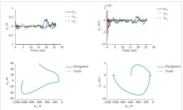
The performance of the navigation system is shown in Figs. 5 to 7. In this case, the thrusters are of and both target and chaser vehicles are initially in the same neighborhood (Table 5). Figure 5 shows the relative position and relative velocity between the vehicles during simulation. Figure 6 depicts how accurately the navigation system can estimate the chaser’s relative position and velocity. Form this i gure, the i lter is able to converge within few minutes and the relative position and velocity can be accurately estimatedwithin the accuracy of the sensors. h e attitude navigation errors and the PD control tracking performance are shown in Fig. 7. As indicated by this i gure, the chaser attitude navigation system is able to converge quickly and the chaser attitude PD controller can track the target attitude and angular velocity trajectories.
h e basic glidelope rendezvous and close proximity operations scenario used to evaluate the performance of the entire closed-loop relative position and attitude control system with the navigation i lter consists of two main segments: the inbound and theoutbound segments. Each segment of the glideslope is followed by 3 minutes of station keeping. First, the inbound segment: the chaser starts to approach the target form [58-580 0] m behind the target and ends at [0-100 0] m. At er 3 minutes
Parameter Value
Initial Relative Position and Velocity
Uncertainties
Process Noise
Measurements Noise
Simulation Step 0.1 s
Measurements
Update 1 Hz
Table 4. Navigation Filter Parameters.
Parameter Target Chaser
a,km 6723.2576 6723.2576
e 0.1 0.1
i, deg 51.6467 51.6467
Ω,deg 188. 0147 188. 0147
ω,deg 174.3022 174.3022
f,deg 270.0882 270.0832
of station keeping at -100 m behind the target, the chaser starts to depart away from the target and leading to a new location -1000 m behind the target. h e chase then stays at rest at that location for another 3 minutes. h e results of this scenario are shown in Figs. 8 and 9. In all of these i gures, dif erent segments of the glideslope are shown, and the variations of in-plane relative motion of the chaser with respect to target vehicle are presented. Figure 8 shows the relative position and velocity plots of relative motion along with the required in order to achieve this trajectory maneuver, while Fig. 9 shows the error in relative position and velocity between the truth model and the navigation model. In all of the above glideslopes, the overall performance of the rendezvous and proximity operations are satisfactory.
h e continuous thrust is calculated using the estimated relative position and velocity, either from the Kalman i lter or from the knowledge of initial conditions, not from the true relative position and velocity of the chaser. As such, the chaser is not expected to reach its intended place exactly, but in the neighborhood thereof. Aided by the sensors, the initial estimation errors subside to an optimal level, determined by the ratio of the process noise matrix , and the measurement noise matrix ,earlier dei ned. Because of the active range and the angle measurements from the LIDAR system, and relatively small measurement errors, the true and the estimated relative position and velocity states are almost indistinguishable, as seen in previous i gures during the steady state.
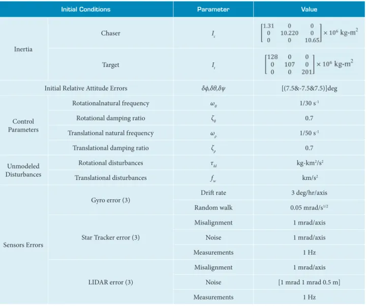
Initial Conditions Parameter Value
Inertia
Chaser Ic
Target It
Initial Relative Attitude Errors δϕ,δθ,δψ [(7.5&-7.5&7.5)]deg
Control Parameters
Rotationalnatural frequency ωθ 1/30 s-1
Rotational damping ratio ζθ 0.7
Translational natural frequency ωρ 1/50 s-1
Translational damping ratio ζρ 0.7
Unmodeled Disturbances
Rotational disturbances τId kg-km2/s2
Translational disturbances fw km/s2
Sensors Errors
Gyro error (3)
Drit rate 3 deg/hr/axis
Random walk 0.05 mrad/s1/2
Star Tracker error (3)
Misalignment 1 mrad/axis
Noise 1 mrad/axis
Measurements 1 Hz
LIDAR error (3)
Misalignment 1 mrad/axis
Noise [1 mrad 1 mrad 0.5 m]
Measurements 1 Hz
ρ
, m
ρY, m
ρX
, m
200
0
-200
-400
-600
-800
0 5 10 15
Time, min
20 25 30
60
40
20
0
-20
-40
-640 -630 -620 -610 -600 -590 -580
ρ
, m/s
0.1
0.05
0
-0.05
-0.1
0 5 10 15 20 25 30
∆V
, m/s
1
0.5
0
-0.5
-1
0 5 10 15 20 25 30
Time, sec Time, sec
ρX ρY
ρZ
ρX ρY ρZ
∆X
∆Y
∆Z
Figure 5. Relative Motion Without.
ρY, m ρY, m
5
0.2
0.1
0
-0.1
-0.2
0 10 20 30
200
150
100
50
0
-50
-700 -650 -600 -550
0.05
0.
-0.05
-0.1
-0.15
-0.2
-700 -650 -600 -550
0
-5
0 5 10 15 20 25
Time, min Time, min
ρY
, m/s
ρX
, m/s
ρe
, m/s ρ, m/se
ρeX ρeY ρeZ
ρeX ρeY ρeZ
Navigation Truth
Navigation Truth
6x 10- 2
- 0 . 1
- 0 . 2 0 0 . 1 4
2
0
- 2
- 4
0 1 0 2 0
Time, min
30
0 10 20
Time, min15 25
5 δω C , d eg/s C h as er E u ler A n g le s E rr o rs, d eg δωCX δωCY δωCZ δΦC δΨC δθC 0.1 0.05 0 -0.05 -0.1 10 5 0 -5 -10
0 10 20
Time, min
30
0 10 20
Time, min 30
An gu la r V el o ci ty T ra ck in g E rr o rs, d eg/s A lt it ude T ra ck in g E rror s, d eg δωCX δωCY δωCZ δΦ δΨ δθ
Figure 7. Chaser Attitude Navigation and Control Performance.
5 0 0 6 0
4 0 20 0 -20 -40 -60 5 0.02 0.01 0 -0.01 -0.02 -0.03 -0.04 0 -5 -10 0 -500 -1000 -1500
0 5 10 15 20 25 30 -1200-1000 -800 -600 -400 -200 0
Time, min
0 5 10 15 20 25 30
Time, sec 0 5 10Time, sec15 20 25 30
ρX
, m
ρY, m
ρ , m/s ∆V , m/s ρ , m ρX ρY ρZ ρX ρY ρZ ∆VX ∆VY ∆VZ
CONCLUSION
h e results of this study indicate that the proposed linear model is clearly ef ective at estimating the relative position and velocity and controlling the relative trajectory. In addition, this model is not restricted to a circular orbit but it can be used as well for an eccentric orbit. Furthermore, by using this model, simple guidance algorithms for glideslope are developed to autonomously approach and depart form a target vehicle. h e relative navigation in this study is utilizing range, azimuth, and
elevation measurements of the target relative to the chaser froma simulated LIDAR system, along with the star tracker and gyro measurements of the chaser and an extended Kalman i lter. h e vehicle attitude dynamics, attitude tracking control, attitude determination, and uncertainties like measurement biases and sensor misalignments are considered in this study to i re the thrusters in the right direction and spin the momentum wheels at the proper rate in the chaser coordinate frame. h e analyst must consider, in addition, of nominal situations, limitations and operational range of the sensors, and limitations of the actuators. h ese topics and others will be addressed in the future.
x 10-2
5
0
-5
-10
5
0
-5
-10
0 5 10 15 20 25 30
Time, min
ρe
, m/s
ρY
, m/s
-1200-1000 -800 -600 -400 -200 0
ρY, m
ρeX ρeY ρeZ
Navigation Truth 1
60
20
-20
-60 40
0
-40 0.5
0
-0.5
-1
0 5 10 15 20 25 30
-1200-1000 -800 -600 -400 -200 0
Time, min
ρe
, m
ρY, m
ρX
, m
ρeX ρeY ρeZ
Navigation Truth
Figure 9. Relative Motion Navigation and Control Performance (Summary Scenario).
REFERENCES
Brown, R.G. and Hawag, P., 1997, “Introduction to Random Signals
and Applied Kalman Filtering”, 3rd Edition, John Wiley & Son Inc.,
United States.
Broucke, R.A., 2003, “Solution of the Elliptic Rendezvous Problem with the Time as Independent Variable”, Journal of Guidance, Control, and Dynamics,Vol. 26, No. 4, pp. 615-621. doi: 10.2514/2.5089.
Carter,T.E., 1998, “State Transition Matrices for Terminal Rendezvous Studies: Brief Survey and New Example”, Journal of Guidance, Control, and Dynamics, Vol. 21, No. 1, pp. 148-155.doi: 10.2514/2.4211.
Clohessy, W.H. and Wiltshire, R.S., 1960, “Terminal Guidance System for Satellite Rendezvous”, Journal of the Aerospace Sciences, Vol. 27, No. 9, pp. 653–678.
Crassidis, J.L. and Junkins, J.L., 2004, “Optimal Estimation of Dynamic System”, 1st Edition, CRC Press LLC, United States.
Fehse, W., 2003, “Automated Rendezvous and Docking of Spacecraft”, 1st Edition, Cambridge University Press, United Kingdom.
Inalhan, G., Tillerson, M., and How, J. P., 2002, “Relative Dynamics and Control of Spacecraft Formation in Eccentric Orbits”, Journal of Guidance, Control, and Dynamics,Vol. 25, No. 1, pp. 48-58.
Jenkins, S.C. and Geller, D.K., 2007, “State Estimation and Targeting For Autonomous Rendezvous and Proximity Operations”, AAS 07-316, Proceedings of theAIAA/AASAstrodynamics Specialists Conference, Mackinac Island, MI.
Junkins, J.L., Kim, S., Crassidis, L., Cheng, Y., and Fosbury, A.M., 2005,“Kalman Filtering for Relative Spacecraft Attitude and Position Estimation”, AIAA 2005-6087, Proceedings of the AIAA Guidance, Navigation, and Control Conference, San Francisco, California.
Lear, W.M., 1985, “Kalman Filtering Techniques”, NASA Johnson Space Center: Mission Planning andAnalysis Division, Houston, TX, JSC-20688.
Melton, R.G., 2000, “Time-Explicit Representation of Relative Motion Between Elliptica lOrbits” Journal of Guidance, Control and Dynamics, Vol. 23, No. 4, pp. 604–610.doi: 10.2514/2.4605.
Sengupta, P. and Vadali, S.R., 2007, “Relative Motion and the Geometry of Formations in KeplerianElliptic Orbits with Arbitrary Eccentricity”, Journal of Guidance, Control, and Dynamics,Vol. 30, No. 4, pp. 953-964.doi: 10.2514/1.25941.
Schaub, H. and Junkins, J.L., 2003, “Analytical Mechanics of Space Systems”, American Institute of Aeronautics and Astronautics, Reston, Virginia, United States.
Tschauner, J. and Hempel, P., 1965, “Rendezvous zueinem in Elliptischer Bahn Umlaufenden Ziel”, ActaAstronautica, Vol. 11, pp. 104-109.
Vallado, D.A., 2001, “Fundamentals of Astrodynamics and Applications”, 2nd Edition, Microcosm Press, El Segundo, California.
Wofinden, D.C. and Geller, D.K., 2007, “Navigating the Road to Autonomous Orbital Rendezvous”, Journal of Spacecraft and Rockets, Vol. 44, No. 4, 2007, pp. 898–909.doi: 10.2514/1.30734.
Wofinden, D.C. and Geller, D.K., 2007, “Relative Angles-Only Navigation and Pose Estimation for Autonomous Orbital Rendezvous”, Journal of Guidance, Control and Dynamics, Vol. 30, No.5, pp. 1455-1469.doi: 10.2514/1.28216.
Wofinden, D.C., 2004, “On-Orbit Satellite Inspection Navigation and Analysis”, M.S. Thesis, Aeronautics and Astronautics Department,Massachusetts Institute of Technology, Cambridge, MA, United States.
Wie, B., 1998,“Space Vehicle Dynamics and Control”, American Institute of Aeronautics and Astronautics, Reston, Virginia, United States.