The simple two-dimensional parameterisation for Flux Footprint Predictions FFP

(1)

GMDD

8, 6757–6808, 2015

Two-dimensional parameterisation for

Flux Footprint Predictions

N. Kljun et al.

Title Page

Abstract Introduction

Conclusions References

Tables Figures

◭ ◮

Back Close

Full Screen / Esc

Printer-friendly Version Interactive Discussion

Discussion

P

a

per

|

Discussion

P

a

per

|

Discussion

P

a

per

|

Discussion

P

a

per

|

Geosci. Model Dev. Discuss., 8, 6757–6808, 2015 www.geosci-model-dev-discuss.net/8/6757/2015/ doi:10.5194/gmdd-8-6757-2015

This discussion paper is/has been under review for the journal Geoscientific Model Development (GMD). Please refer to the corresponding final paper in GMD if available.

The simple two-dimensional

parameterisation for Flux Footprint

Predictions FFP

N. Kljun1, P. Calanca2, M. W. Rotach3, and H. P. Schmid4

1

Department of Geography, Swansea University, Swansea, United Kingdom

2

Agroscope, Institute for Sustainability Sciences, Zurich, Switzerland

3

Institute of Atmospheric and Cryospheric Sciences, Innsbruck University, Innsbruck, Austria

4

KIT, Institute of Meteorology and Climate Research, Garmisch-Partenkirchen, Germany Received: 2 July 2015 – Accepted: 11 August 2015 – Published: 24 August 2015

Correspondence to: N. Kljun ([email protected])

(2)

GMDD

8, 6757–6808, 2015

N. Kljun et al.

Title Page

Tables Figures

◭ ◮

Back Close

Full Screen / Esc

Discussion

P

a

per

|

Discussion

P

a

per

|

Discussion

P

a

per

|

Discussion

P

a

per

|

Abstract

Flux footprint models are often used for interpretation of flux tower measurements, to estimate position and size of surface source areas, and the relative contribution of passive scalar sources to measured fluxes. Accurate knowledge of footprints is of crucial importance for any upscaling exercises from single site flux measurements to

5

ecosystem or regional scale. Hence, footprint models are ultimately also of consid-erable importance for improved greenhouse gas budgeting. With increasing numbers of flux towers within large monitoring networks such as FLUXNET, ICOS, NEON, or AMERIFLUX, and with increasing temporal range of observations from such towers (order of decades) and availability of airborne flux measurements, there has been an

10

increasing demand for reliable footprint estimation. Even though several sophisticated footprint models have been developed in recent years, most are still not suitable for application to long time series, due to their high computational demands. Existing fast footprint models, on the other hand, are based on Surface Layer theory and hence are of restricted validity for real case applications.

15

To remedy such shortcomings, we present the two-dimensional Flux Footprint Pa-rameterisation, FFP, based on a novel scaling approach for the crosswind distribution of the flux footprint and on an improved version of the footprint parameterisation of Kljun et al. (2004b). Compared to the latter, FFP now provides not only the extent, but also the width and shape of footprint estimates, and explicit consideration of the eff_{ects of} 20

the surface roughness length. The footprint parameterisation has been developed and evaluated using simulations of the backward Lagrangian stochastic particle dispersion model LPDM-B (Kljun et al., 2002). Like LPDM-B, the parameterisation is valid for a broad range of boundary layer conditions and measurement heights over the entire planetary boundary layer. Thus it can provide footprint estimates for a wide range of

25

real case applications.

The new footprint parameterisation requires inputs that can be easily determined from, for example, flux tower measurements or airborne flux data. FFP can be applied

(3)

GMDD

8, 6757–6808, 2015

N. Kljun et al.

Title Page

Tables Figures

◭ ◮

Back Close

Full Screen / Esc

Discussion

P

a

per

|

Discussion

P

a

per

|

Discussion

P

a

per

|

Discussion

P

a

per

|

to data of long-term monitoring programmes as well as be used for quick footprint estimates in the field, or for designing new sites.

1 Introduction

Flux footprint models are used to describe the spatial extent and position of the surface area that is contributing to a turbulent flux measurement at a specific point in time, for

5

specific atmospheric conditions and surface characteristics. They are hence very im-portant tools when it comes to interpretation of flux measurements of passive scalars, such as the greenhouse gases carbon dioxide (CO₂), water vapour (H₂O), or methane (CH₄).

In recent years, the application of footprint models has become a standard task in

10

analysis of measurements from flux towers (e.g., Aubinet et al., 2001; Rebmann et al., 2005; Nagy et al., 2006; Göckede et al., 2008; Mauder et al., 2013) or airborne flux measurements (Kustas et al., 2006; Mauder et al., 2008; Hutjes et al., 2010; Metzger et al., 2012) of inert (i.e., long-lived) greenhouse gases. Information about the sink and source location is even more crucial for towers in heterogeneous or disturbed

land-15

scapes (e.g., Sogachev et al., 2005), a topical study area in recent times. Schmid (2002) showed that the use of the footprint concept has been increasing exponention-ally since 1972. Since then, footprint models have been used for planning and design of new flux towers and have been applied to most flux tower observations around the globe, to support the interpretation of such measurements.

20

Long-term and short-term flux observations are exposed to widely varying atmo-spheric conditions and their interpretation therefore involves an enormous amount of footprint calculations. Despite the widespread use of footprint models, the selection of a suitable model still poses a major challenge. Complex footprint models based on Large Eddy Simulations (LES; e.g., Luhar and Rao, 1994; Leclerc et al., 1997;

Stein-25

(4)

GMDD

8, 6757–6808, 2015

N. Kljun et al.

Title Page

Tables Figures

◭ ◮

Back Close

Full Screen / Esc

Discussion

P

a

per

|

Discussion

P

a

per

|

Discussion

P

a

per

|

Discussion

P

a

per

|

(LS; e.g., Leclerc and Thurtell, 1990; Horst and Weil, 1992; Flesch, 1996; Baldocchi, 1997; Rannik et al., 2000; Kljun et al., 2002; Hsieh et al., 2003) can, to a certain de-gree, off_{er the ability to resolve complex flow structures (e.g., flow over a forest edge)}

and surface heterogeneity. However, to date they are laborious to run, still highly CPU-intensive, and hence can in practice be applied only for case studies over selected

5

hours or days, and most are constrained to a narrow range of atmospheric conditions. These complex models are not suited for dealing with the vast increase of long-term flux tower data or the more and more frequent airborne flux measurements. Instead, quick footprint estimates are needed, models that can deal with large amounts of input data, for example several years of half-hourly data points at several observational levels

10

at multiple locations. For these reasons, analytical footprint models are often used as a compromise (e.g., Schuepp et al., 1990; Leclerc and Thurtell, 1990; Schmid and Oke, 1990; Wilson and Swaters, 1991; Horst and Weil, 1992, 1994; Schmid, 1994, 1997; Haenel and Grünhage, 1999; Kormann and Meixner, 2001). These models are simple and fast, but their validity is often constrained to ranges of receptor heights and

bound-15

ary layer conditions that are much more restricted than those commonly observed. Existing footprint modelling studies off_{er the potential for simple parameterisations}

as, for example, proposed by Horst and Weil (1992; 1994), Weil and Horst (1992), Schmid (1994) or Hsieh et al. (2000). The primary drawback of these parameterisations is their limitation to a particular turbulence scaling domain (often Surface Layer scaling),

20

or to a limited range of stratifications. Conversely, measurement programs of even just a few days are regularly exposed to conditions spanning several turbulence scaling domains.

To fill this gap, Kljun et al. (2004b) introduced a footprint parameterisation based on a fit to scaled footprint estimates derived from the Lagrangian stochastic particle

dis-25

persion model LPDM-B (Kljun et al., 2002). LPDM-B is one of very few LS footprint models valid for a wide range of boundary layer stratifications and receptor heights. Likewise, the parameterisation of LPDM-B is also valid for outside Surface Layer con-ditions and for non-Gaussian turbulence, as for example for the Convective

(5)

GMDD

8, 6757–6808, 2015

N. Kljun et al.

Title Page

Tables Figures

◭ ◮

Back Close

Full Screen / Esc

Discussion

P

a

per

|

Discussion

P

a

per

|

Discussion

P

a

per

|

Discussion

P

a

per

|

ary Layer. However, the parameterisation of Kljun et al. (2004b) comprises only the crosswind-integrated footprint, i.e. it describes the footprint function’s upwind extent but not its width.

In recent time, footprint model outputs have frequently been combined with surface information, such as remote sensing data (e.g., Schmid and Lloyd, 1999; Kim et al.,

5

2006; Li et al., 2008; Barcza et al., 2009; Chasmer et al., 2009; Sutherland et al., 2014). As remote sensing data is increasingly available in high spatial resolution, a footprint often covers more than one pixel of remote sensing data; hence there is a need for information of the crosswind spread of the footprint. Similar to FSAM (Schmid, 1994), the footprint model of Kormann and Meixner (2001) includes dispersion in crosswind

10

direction. Detto et al. (2006) provided a crosswind extension of the footprint model of Hsieh et al. (2000). However, all these models are of limited validity restricted to measurements close to the surface. For more details on their validity and restrictions, and for a comprehensive review on existing footprint techniques and approaches the reader is referred to Schmid (2002), Vesala et al. (2008), or Leclerc and Foken (2014).

15

This study addresses the issues and shortcomings mentioned above. We present the new footprint parameterisation FFP, with improved footprint predictions for elevated measurement heights in stable stratifications. The influence of the surface roughness has been implemented into the scaling approach explicitly. Further and most impor-tantly, the new parameterisation describes also the crosswind spread of the footprint

20

and hence, it is suitable for many practical applications. Like all footprint models that do not simulate the full time- and space-explicit flow, FFP implicitely assumes sta-tionarity over the eddy-covariance integration period (typically 30 min) and horizontal homogeneity of the flow (but not of the scalar source/sink distribution). As in Kljun et al. (2004b), the new parameterisation is based on a scaling approach of flux footprint

re-25

(6)

GMDD

8, 6757–6808, 2015

N. Kljun et al.

Title Page

Tables Figures

◭ ◮

Back Close

Full Screen / Esc

Discussion

P

a

per

|

Discussion

P

a

per

|

Discussion

P

a

per

|

Discussion

P

a

per

|

2 Footprint dataset

Mathematically, the flux footprint,f, is the transfer function between sources or sinks of passive scalars at the surface,Q_c, and the turbulent flux,F_c, measured at a receptor at heightzm(e.g., Pasquill and Smith, 1983; Schmid, 2002). We define a local footprint coordinate system, where the receptor is mounted above the origin (0, 0) and positive

5

xindicates upwind distance, such that

F_c(0, 0,z_m)=

Z

ℜ

Q_c(x,y)f(x,y) dxdy, (1)

where_ℜ denotes the integration domain. As the footprint function is always specific to a given measurement height, the vertical reference inf is neglected, for simplicity. It follows that the footprint function is proportional to the flux increment arising from a

10

single unit point source or sink,Q_u, i.e.,

f(x,y)=Fc(0, 0,zm)

Q_u(x,y) . (2)

As Fc is a flux density (per unit area) and Qu is a source or sink integrated over a unit area, the two-dimensional footprint function has the dimension of [1/area]. Assum-ing that crosswind turbulent dispersion can be treated independently from vertical or

15

streamwise transport, the footprint function can be expressed in terms of a crosswind-integrated footprint,fy_{, and a crosswind dispersion function,}_D

y, (see, e.g., Horst and Weil, 1992)

f(x,y)=_fy₍_x₎_D

y. (3)

Derivation and evaluation of the footprint parameterisation are based on footprint

20

calculations using LPDM-B (Kljun et al., 2002). LPDM-B is a footprint model of the

(7)

GMDD

8, 6757–6808, 2015

N. Kljun et al.

Title Page

Tables Figures

◭ ◮

Back Close

Full Screen / Esc

Discussion

P

a

per

|

Discussion

P

a

per

|

Discussion

P

a

per

|

Discussion

P

a

per

|

Lagrangian stochastic particle dispersion type, with three-dimensional dispersion of in-ert particles as described by Rotach et al. (1996) and de Haan and Rotach (1998). LPDM-B fulfils the well-mixed condition (Thomson, 1987) and is valid for stable, neu-tral, and convective boundary layer stratifications, assuming stationary flow conditions. It has been shown to reproduce wind-tunnel simulations very well (Kljun et al., 2004a).

5

LPDM-B tracks particles backward in time, from the receptor location to the source / sink, at the surface (i.e., particle touchdown location, see Kljun et al., 2002, for details). Hence, footprint calculation can be based on all computed particle tracks directly with-out the need for coordinate transformation. We refer to Rotach et al. (1996), de Haan and Rotach (1998), and Kljun et al. (2002) for details in the formulation and evaluation

10

of the model.

Compared to the original parameterisation of Kljun et al. (2004b), we have increased the parameter space for LPDM-B simulations especially for stable boundary layer con-ditions. We also increased the covered range of roughness lengths, z₀, to include roughness lengths that may be found over sparse forest canopies. For the

parame-15

terisation, a total of 200 simulations were run with LPDM-B for measurement heights between 1 and 1000 m and boundary layer conditions between strongly convective, neutral, to strongly stable. With that, the simulations span a range of stability regimes, namely the Surface Layer, Local Scaling Layer, Z-less Scaling Layer, Neutral Layer, the Free Convection Layer, and the Mixed Layer (cf. Holtslag and Nieuwstadt, 1986).

20

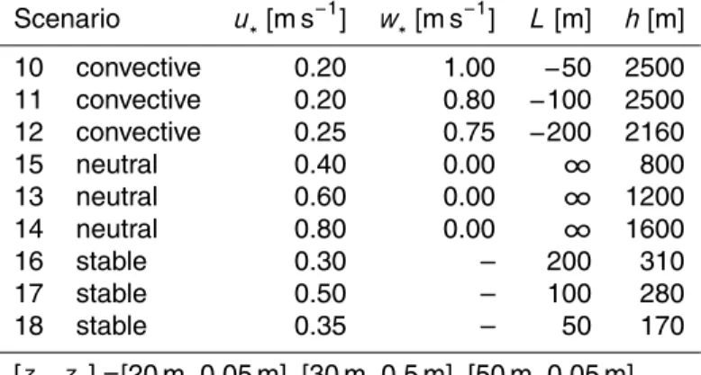
Table 1 gives an overview of the parameter space for the simulated scenarios. We use standard definitions for the friction velocity, u_∗, the convective velocity scale, w_∗, and the Obukhov length, L (see, e.g., Stull, 1988, and Appendix B for details and for the definition of L). Each scenario was run for the whole set of roughness lengths and for all listed measurement heights. Note that we define the measurement height as

25

(8)

GMDD

8, 6757–6808, 2015

N. Kljun et al.

Title Page

Tables Figures

◭ ◮

Back Close

Full Screen / Esc

Discussion

P

a

per

|

Discussion

P

a

per

|

Discussion

P

a

per

|

Discussion

P

a

per

|

of the roughness elements, approximated byhrs=10z0 (Grimmond and Oke, 1999)]. Here, we usez_∗=_2.75_h

rs.

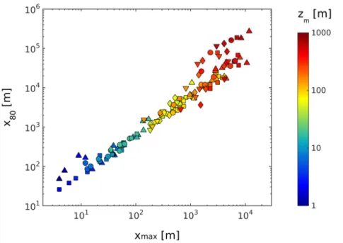
As expected for such a broad range of scenarios, the resulting footprints of LPDM-B simulations show a vast range of extents and sizes. Fig. 1 depicts this range by means of peak location of the footprints and their extent, when integrated from their

5

peak to 80 % contribution of the total footprint (cf. Sect. 5.3). For example, the 80 % footprint extents ranged from a few tens to a few hundreds of meters upwind of the tower location for the lowest measurement heights. For the highest measurements, the 80 % footprints ranged up to 270 km.

An additional set of 27 LPDM-B simulations was run for independent evaluation of

10

the footprint parameterisation. Measurement heights that are typical for flux tower sites were selected for this evaluation set, with boundary layer conditions again ranging from convective to stable. Table 2 lists the characteristics of these additional scenarios.

3 Scaling of footprints

The vast range in footprint sizes presented above clearly manifests that it is not

prac-15

tical to fit a single footprint parameterisation to all real-scale footprints. An additional step of footprint scaling is hence needed, with the goal of deriving a universal non-dimensional footprint. Ideally, such dimensionless footprints collapse to a single shape or narrow ensemble of curves. We follow a method that borrows from BuckinghamΠ

dimensional analysis (e.g., Stull, 1988), using dimensionlessΠ_{-functions to scale the} 20

footprint estimates of LPDM-B, similar to Kljun et al. (2004b), and scale the two com-ponents of the footprint, the crosswind-integrated footprint and its crosswind dispersion (Eq. 3), in two separate steps.

(9)

GMDD

8, 6757–6808, 2015

N. Kljun et al.

Title Page

Tables Figures

◭ ◮

Back Close

Full Screen / Esc

Discussion

P

a

per

|

Discussion

P

a

per

|

Discussion

P

a

per

|

Discussion

P

a

per

|

3.1 Scaled crosswind-integrated footprint

As in Kljun et al. (2004b), we choose scaling parameters relevant for the crosswind-integrated footprint function, fy₍_x_{). The first choice is the receptor height,} _z

m, as ex-perience shows that the footprint (both its extent and footprint function value) is most strongly dependent on this height. Secondly, as indicated in Eq. (2), the footprint is

5

proportional to the flux at height z_m. We hence formulate another scaling parame-ter based on the common finding that turbulent fluxes decline approximately linearly through the planetary boundary layer, from their surface value to the boundary layer height,h, where they disappear (e.g., Stull, 1988). Lastly, as a transfer function in tur-bulent boundary layer flow, the footprint is directly aff_{ected by the mean wind velocity} 10

at the measurement height,u(zm), as well as by the surface shear stress, represented by the friction velocity, u_∗. The well-known diabatic Surface Layer wind speed profile (e.g., Stull, 1988) relatesu(z_m) to the roughness length,z₀, and the integrated form of the non-dimensional wind shear,Ψ

M, that accounts for the effect of stability (zm/L) on the flow.

15

With the above scaling parameters we form four dimensionlessΠ_{groups as}

Π

1=fyzm

Π

2=

x zm

Π

3=

h₋z_m h =1−

z_m h

Π

4=

u(zm)

u_∗ k=ln

_z m

z₀

−Ψ

M (4)

(10)

GMDD

8, 6757–6808, 2015

N. Kljun et al.

Title Page Abstract Introduction Conclusions References Tables Figures ◭ ◮ ◭ ◮ Back Close

Full Screen / Esc

Printer-friendly Version Interactive Discussion Discussion P a per | Discussion P a per | Discussion P a per | Discussion P a per |

wherek=_{0.4 is the von Karman constant. We use} Ψ

M as suggested by Högström (1996): Ψ M=    −5.3zm

L forL >0,

ln1+₂χ2+_{2 ln}1+χ

2

−2tan−1(χ)+π

2 forL <0 .

(5)

withχ=₍₁₋₁₉_z

m/L)1

/4_{. In principle,}_Ψ

M is based on Monin-Obukhov similarity and valid within the Surface Layer. Hence special care was taken in testing this scaling

ap-5

proach for measurements outside the Surface Layer (see below). In contrast to Kljun et al. (2004b), the present study incorporates the roughness length directly in the scal-ing procedure: high surface roughness (i.e., largez₀) enhances turbulence relative to the mean flow, and thus shortens the footprints. Here,z0is either directly used as input parameter or is implicitly included through the fraction ofu(z_m)/u_∗.

10

The non-dimensional form of the crosswind-integrated footprint,Fy∗, can be written as a yet unknown functionϕof the non-dimensional upwind distance,X∗. ThusFy∗= ϕ(X∗), withX∗= Π

2Π3Π− 1 4 andF

y∗_{= Π}

1Π− 1

3 Π4, such that

X∗= x z_m

1₋zm

h

_u₍_z m)

u_∗ k

!−1

(6)

= x

z_m

1₋zm

h ln

_z m

z₀

−Ψ_M

−1

(7)

15

Fy∗=_fy_z m

1₋zm

h

−1 _u₍_z m)

u_∗ k (8)

=_fy_z m

1₋zm

h −1 ln _z m z₀ −Ψ M . (9)

As a next step, the above scaling procedure is applied to all footprints of Scenar-ios 1 to 8 (Table 1) derived by LPDM-B. Despite the huge range of footprint extents

(11)

GMDD

8, 6757–6808, 2015

N. Kljun et al.

Title Page

Tables Figures

◭ ◮

Back Close

Full Screen / Esc

Discussion

P

a

per

|

Discussion

P

a

per

|

Discussion

P

a

per

|

Discussion

P

a

per

|

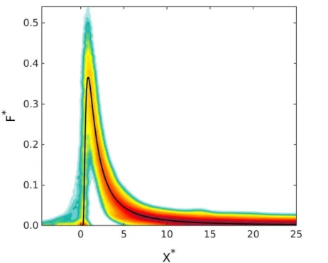
(Fig. 1), the resulting scaled footprints collapse into an ensemble of footprints of very similar shape, peak location, and extent (Fig. 2). Hence the new scaling procedure for crosswind-integrated flux footprints proves to be successful across the whole range of simulations, including the large range of surface roughness lengths and stability regimes.

5

3.2 Scaled crosswind dispersion

Crosswind dispersion can be described by a Gaussian distribution function withσ_y as the standard deviation of the crosswind distance (e.g., Pasquill and Smith, 1983). In contrast to vertical dispersion, Gaussian characteristics are valid for crosswind disper-sion for the entire stability range and are even appropriate over complex surfaces (e.g.,

10

Rotach et al., 2004). The three-dimensional particle dispersion of LPDM-B incorpo-rates the Gaussian lateral dispersion (cf. Kljun et al., 2002). Note that variations of the mean wind direction by the Ekman eff_{ect are neglected. Hence, assuming Gaussian}

characteristics for the crosswind dispersion function,D_y, in Eq. (3), the flux footprint,

f(x,y), can be described as (e.g., Horst and Weil, 1992)

15

f(x,y)=_fy₍_x₎ 1 √

2πσ_y exp − y2

2σ_y2

!

. (10)

Here,y is the crosswind distance from the centreline (i.e., the x-axis) of the footprint. The standard deviation of the crosswind distance,σy, depends on boundary layer con-ditions and the upwind distance from the receptor.

Similar to the crosswind-integrated footprint, we aim to derive a scaling approach

20

(12)

GMDD

8, 6757–6808, 2015

N. Kljun et al.

Title Page

Tables Figures

◭ ◮

Back Close

Full Screen / Esc

Discussion

P

a

per

|

Discussion

P

a

per

|

Discussion

P

a

per

|

Discussion

P

a

per

|

therefore set

Π

5=

y z_m

Π

6=

σy

z_m

Π

7=

σ_v

u_∗. (11)

In analogy to, for example, Nieuwstadt (1980), we define a non-dimensional standard

5

deviation of the crosswind distance,σy∗, proportional to Π6Π−71. The non-dimensional crosswind distance from the receptor,Y∗, is linked toσy∗ through Eq. (10) and accord-ingly has to be proportional toΠ

5Π−71. With that

Y∗=_p

s1

y z_m

u_∗

σ_v (12)

σ_y∗=_p

s1

σ_y z_m

u_∗ σv

, (13)

10

where p_s1 is a proportionality factor depending on stability. Based on the LPDM-B results, we set p_s1=_min(1,z_m/L

−

1

10−5+_p_{), with} _p=_{0.8 for} _L_≤_{0 and} _p=_0.55

forL >0, respectively. In Fig. 3 unscaled distance from the receptor, x, and scaled, non-dimensional distanceX∗are plotted against the unscaled and scaled deviations of the crosswind distance, respectively (see Appendix C for information on the derivation

15

ofσ_y from LPDM-B simulations). The scaling procedure is clearly successful, as the scaled deviation of the crosswind distance,σy∗, of all LPDM-B simulations collapse into a narrow ensemble when plotted againstX∗(Fig. 3, right-hand panel). For largeX∗, the ensemble spread increases mainly due to increased scatter of LPDM-B simulations for distances far away from the receptor.

20

(13)

GMDD

8, 6757–6808, 2015

N. Kljun et al.

Title Page

Tables Figures

◭ ◮

Back Close

Full Screen / Esc

Discussion

P

a

per

|

Discussion

P

a

per

|

Discussion

P

a

per

|

Discussion

P

a

per

|

4 Flux Footprint Parameterisation FFP

The successful scaling of both along-wind and crosswind shapes of the footprint into narrow ensembles within a non-dimensional framework provides the basis for fitting a parameterisation curve to the ensemble of scaled LPDM-B results. Like for the scaling approach, the footprint parameterisation is set up in two separate steps, the

crosswind-5

integrated footprint, and its crosswind dispersion.

4.1 Crosswind-integrated footprint parameterisation

The ensemble of scaled crosswind-integrated footprints Fy∗(X∗) of LPDM-B is suffi

-ciently coherent that it allows fitting a single representative function to it. We choose the product of a power function and an exponential function as a fitting function for the

10

parameterised cross-wind integrated footprint ˆFy∗( ˆX∗):

ˆ

Fy∗=_a_{( ˆ}_X∗₋_d₎b _exp

−c

ˆ

X∗₋_d

. (14)

Derivation of the fitting parameters,a,b,c,d is dependent on the constraint that the integral of the footprint parameterisation (cf. Eq. 14) must equal unity to satisfy the integral conditionR∞

−∞F

y∗₍_X∗₎_{d X}∗₌_{1 (cf. Schmid, 1994; Kljun et al., 2004b). Hence} 15

∞

Z

d ˆ

Fy∗( ˆX∗) d ˆX∗=₁

= ∞

Z

d

a( ˆX∗₋d)b exp

−c

ˆ

X∗₋_d

d ˆX∗ (15)

=_{a c}b+1Γ₍₋_b₋_{1) ,} ₍₁₆₎

whereΓ₍_b_{) is the gamma function, and here}Γ₍₋_b₋₁₎_≡R∞ 0 t−

b−2

(14)

GMDD

8, 6757–6808, 2015

N. Kljun et al.

Title Page

Tables Figures

◭ ◮

Back Close

Full Screen / Esc

Discussion

P

a

per

|

Discussion

P

a

per

|

Discussion

P

a

per

|

Discussion

P

a

per

|

The footprint parameterisation (Eq. 14) is fitted to the scaled footprint ensemble using an unconstrained nonlinear optimization technique based on the Nelder-Mead simplex direct search algorithm (Lagarias et al., 1998). With that, we find

a=_1.452 b=₋_1.991 5

c=_1.462

d=_{0.136 .} ₍₁₇₎

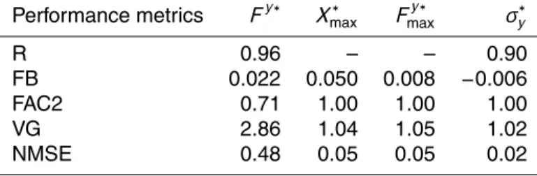
Figure 2 shows that the parameterisation of the crosswind-integrated footprint repre-sents all scaled footprints very well. The goodness-of-fit of this single parameterisation to the ensemble of scaled footprints for all simulated measurement heights, stability

10

conditions, and roughness lengths, is evident from model performance metrics (see, e.g., Hanna et al., 1993; Chang and Hanna, 2004), including the Pearson’s correla-tion coeffi_{cient (R), the fractional bias (FB), the fraction of the parameterisation within}

a factor of two of the scaled footprints (FAC2), the geometric variance (VG), and the normalised mean square error (NMSE). Table 3 lists these performance metrics for the

15

parameterisation of the full extent of the crosswind-integrated footprint curve, for the footprint peak location, and for the footprint peak value of the parameterisation against the corresponding scaled LPDM-B results. The fit can be improved even more if the parameters are optimised to represent footprints of convective or neutral and stable conditions only (see Appendix A).

20

4.2 Parameterisation of the crosswind footprint extent

A single function can be fitted also to the scaled crosswind dispersion. In conformity with Deardorff_{and Willis (1975), the fitting function was chosen to be of the form}

ˆ

σ_y∗ =_a

c

bc( ˆX∗)2 1+_c

cXˆ∗ !1/2

. (18)

(15)

GMDD

8, 6757–6808, 2015

N. Kljun et al.

Title Page

Tables Figures

◭ ◮

Back Close

Full Screen / Esc

Discussion

P

a

per

|

Discussion

P

a

per

|

Discussion

P

a

per

|

Discussion

P

a

per

|

A fit to the data of scaled LPDM-B simulations results in

a_c=_2.17 b_c=_1.66

c_c=_{20.0 .} ₍₁₉₎

The above parameterisation of the scaled deviation of the crosswind distance of the

5

footprint is plotted in Fig. 3 (right panel). The performance metrics confirm that theσy∗ of the scaled LPDM-B simulations are very well reproduced by the parameterisation ˆσ_y∗

(Table 3).

5 Real-scale flux footprint

Typically, users of footprint models are interested in footprints given in a real-scale

10

framework, such that distances (e.g., between the receptor and maximum contribution to the measured flux) are given in metres or kilometers. Depending on the availability of observed parameters, the conversion from the non-dimensional (parameterised) foot-prints to real-scale dimensions can be based on either Eqs. (6) and (8), or on Eqs. (7) and (9). For convenience, the necessary steps of the conversion are described in the

15

following, by means of some examples.

5.1 Maximum footprint contribution

The distance between the receptor and the maximum contribution to the measured flux can be approximated by the peak location of the crosswind-integrated footprint. The maximum’s position can be deduced from the derivative of Eq. (14) with respect to

20 X∗:

ˆ

X_max∗ =−c

(16)

GMDD

8, 6757–6808, 2015

N. Kljun et al.

Title Page

Tables Figures

◭ ◮

Back Close

Full Screen / Esc

Discussion

P

a

per

|

Discussion

P

a

per

|

Discussion

P

a

per

|

Discussion

P

a

per

|

Using the fitting parameters as listed in Eq. (17) to evaluate ˆX_max∗ , the peak location is converted from the scaled to the real-scale framework applying Eq. (6)

x_max=_Xˆ∗

max zm

1₋zm

h

−1 _u₍_z m)

u_∗ k

=_0.87 _z

m

1₋zm

h

−1 _u₍_z m)

u_∗ k, (21)

or, alternatively applying Eq. (7)

5

xmax=Xˆmax∗ zm

1₋zm

h

−1 ln

_z m

z₀

−Ψ

M

=_0.87 _z

m

1₋zm

h

−1 ln

_z m

z0

−Ψ

M

, (22)

withΨ_M _{as given in Eq. (5). Hence} _x

max can easily be derived from observations of

z_m,h, andu(z_m),u_∗, orz₀,L, and the constant value of ˆX_max∗ . For suggestions on how to estimate the planetary boundary layer height,h, if not measured, see Appendix B.

10

5.2 Two-dimensional flux footprint

The two-dimensional footprint function can be calculated by applying the crosswind dispersion (Eq. 10) to the crosswind-integrated footprint. With inputs of the scaling parametersz_m,h,u_∗,σ_v, andu(z_m) orz₀,L, the two-dimensional footprint for any (x,y) combination can be derived easily by the following steps:

15

1. EvaluateX∗using Eq. (6) or (7) for givenx.

2. Derive ˆFy∗and ˆσy∗ by insertingX∗ for ˆX∗in Eqs. (14) and (18).

3. Invert Eqs. (8) or (9) and (13) to derivefy _and_σ

(17)

GMDD

8, 6757–6808, 2015

N. Kljun et al.

Title Page

Tables Figures

◭ ◮

Back Close

Full Screen / Esc

Discussion

P

a

per

|

Discussion

P

a

per

|

Discussion

P

a

per

|

Discussion

P

a

per

|

4. Evaluatef(x,y) for givenxandy using Eq. (10).

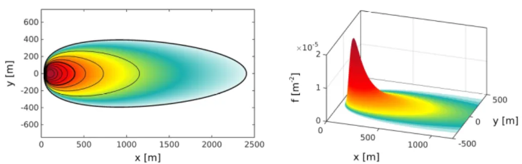
Fig. 4 depicts an example footprint for convective conditions, computed by applying the described approach to arrays of (x,y) combinations.

5.3 Relative contribution to the total footprint area

Often, the interest lies in the extent and location of the area contributing to, for

ex-5

ample, 80 % of the measured flux. For such applications, there are two approaches: (i) the crosswind-integrated footprint function,fy₍_x_{), is integrated from the receptor} lo-cation to the upwind distance where the contribution of interest is obtained; (ii) the two-dimensional footprint functionf(x,y) is integrated from the footprint peak location into all directions along constant levels of footprint values until the contribution of

inter-10

est is obtained. The result is the source area: the smallest possible area containing a given relative flux contribution (cf. Schmid, 1994). This approach can also be used as a one-dimensional equivalent to the source area, for the crosswind-integrated footprint. For case (i) starting at the receptor location, we denote ˆX_R∗ as the upper limit of the footprint parameterisation ˆF∗( ˆX∗) containing the area of interest, i.e. the fraction

15

R of the total footprint (that integrates to 1). The integral of Eq. (14) up to ˆX_R∗ can be simplified (see Appendix D for details) as

R=_exp −c

ˆ

X_R∗−d

!

. (23)

With that, the distance between the receptor and ˆX_R∗ can be determined very simply as

ˆ

X_R∗ = −c

ln(R)+d, (24)

(18)

GMDD

8, 6757–6808, 2015

N. Kljun et al.

Title Page Abstract Introduction Conclusions References Tables Figures ◭ ◮ ◭ ◮ Back Close

Full Screen / Esc

Printer-friendly Version Interactive Discussion Discussion P a per | Discussion P a per | Discussion P a per | Discussion P a per |

and in real-scale

xR=

−c

ln(R)+d

zm

1₋zm

h

−1 _u₍_z m)

u_∗ k

=

−c

ln(R)+d

zm

1₋zm

h −1 ln _z m z₀ −Ψ M , (25)

whereR is a value between 0.1 and 0.99. As the above is based on the crosswind-integrated footprint, the derivation includes the full width of the footprint at any

along-5

wind distance from the receptor.

There is no near-analytical solution for the description of the source area, the extent of the fractionR, when integrating from the peak location (e.g., Schmid, 1994; Kormann and Meixner, 2001). Instead, the size of the source area has to be derived through iterative search. For crosswind-integrated footprints, the downwind ( ˆX_R∗_d<Xˆ_max∗ ) and

10

upwind ( ˆX_max∗ <Xˆ_R∗_u) distance from the receptor including the fractionR can be approx-imated as a function of ˆX_R∗ using LPDM-B results:

ˆ

X_R∗_d,u=_n

1

ˆ

X_R∗n2+_n

3 (26)

For the downwind limit ˆX_R∗_d,n₁=_0.44,_n

2=−0.77,n3=0.24. For the upwind limit, ˆXR∗u, the approximation is split into two parts,n₁=_0.60,_n

2=1.32,n3=0.61 for ˆXmax∗ <XˆR∗ ≤

15

1.5, andn₁=_0.96,_n

2=1.01,n3=0.19 for 1.5<XˆR∗ <∞. The scaled distances ˆX∗,Rd and ˆX_∗_,Rucan again be transformed into real-scale values using Eqs. (6) or (7).

If the size and position of the two-dimensionalR-source area are of interest, but not the footprint function value (i.e. footprint weight) itself, the pairs ofx_R andy_Rdescribing its shape can be drawn from a lookup table of the scaled corresponding X_R∗ and Y_R∗ 20

values. If the footprint function values are needed for weighting of source emissions or sinks, iterative search procedures have to be applied to each footprint. Figure 4 (left panel) illustrates examples of contour lines ofR-fractions from 10 to 90 % of a footprint.

(19)

GMDD

8, 6757–6808, 2015

N. Kljun et al.

Title Page

Tables Figures

◭ ◮

Back Close

Full Screen / Esc

Discussion

P

a

per

|

Discussion

P

a

per

|

Discussion

P

a

per

|

Discussion

P

a

per

|

5.4 Footprint estimates for extended time series

The presented footprint model is computationally inexpensive and hence can be run easily for several years of data in, for example, half-hourly time steps. Each single data point can be associated with its source area by converting the footprint coordinate sys-tem to geographical coordinates, and positioning a discretised spatial array containing

5

the footprint function onto a map or aerial image surrounding the receptor position. In many cases, an aggregated footprint, a so-called footprint climatology, is of more interest to the user than a series of footprint estimates. The aggregated footprint can be normalised and presented for several levels of relative contribution to the total ag-gregated footprint. Figure 5 shows an example of such a footprint climatology for one

10

month of half-hourly input data for the ICOS flux tower site Norunda in Sweden (cf. Lin-droth et al., 1998). A footprint climatology can be derived for selected hours of several days, for months, seasons, years, etc., depending on interest.

Combined with remotely sensed data, a footprint climatology provides spatially ex-plicit information on vegetation structure, topography, and possible source/sink

influ-15

ences on the measured fluxes. This additional information has proven to be beneficial for analysis and interpretation of flux data (e.g., Rahman et al., 2001; Rebmann et al., 2005; Kim et al., 2006; Chasmer et al., 2008; Barcza et al., 2009; Gelybó et al., 2013). A combination of the footprint parameterisation presented here with high-resolution remote sensing data can be used not only to estimate the footprint area for

measure-20

ments, but also to weigh or classify spatially continuous information on the surface and vegetation for its impact on measurements.

Certain remotely sensed data, for example airborne LiDAR data, allow for approxi-mate derivation of the surface roughness length (Chasmer et al., 2008). Alternatively,

z₀may be estimated from flux tower measurements (e.g., Kim et al., 2006). Ifz₀varies

25

substantially for diff_{erent wind directions, we suggest running a spin-up of the footprint}

(20)

GMDD

8, 6757–6808, 2015

N. Kljun et al.

Title Page

Tables Figures

◭ ◮

Back Close

Full Screen / Esc

Discussion

P

a

per

|

Discussion

P

a

per

|

Discussion

P

a

per

|

Discussion

P

a

per

|

of the footprints is reached. We recommend such a spin-up procedure despite the fact that footprint models are in principle not valid for non-scalars, such as momentum.

6 Discussion

6.1 Evaluation of FFP and sensitivity to input parameters

Exhaustive evaluation of footprint models is still a diffi_{cult task, and clearly, tracer-flux} 5

field experiments would be very helpful. We are aware that in reality such experiments are both challenging and expensive to run. However, the aim of the present study is not to present a new footprint model, but to provide a simple and easily accessible parameterisation or “short-cut” for the much more sophisticated, but highly resource intensive, Lagrangian stochastic particle dispersion footprint model LPDM-B of Kljun

10

et al. (2002). For the current study, we hence restrict the assessment of the presented footprint parameterisation to an evaluation against an additional set of LPDM-B simu-lations. A description of these additional scenarios can be found in Table 2.

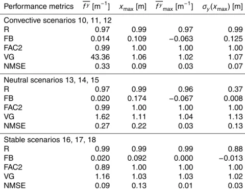
The capability of the footprint parameterisation to reproduce the real-scale footprint of LPDM-B simulations is tested by means of the full extent of the footprint, its peak

15

location, peak value, and its crosswind dispersion. Performance metrics show that for all stability classes (convective, neutral, and stable scenarios), the footprint parame-terisation is able to predict the footprints simulated by the much more sophisticated Lagrangian stochastic particle dispersion model very accurately (Table 4).

Results shown here clearly demonstrate that our objective of providing a short-cut

20

to LPDM-B has been achieved. The full model was tested successfully against wind tunnel data (Kljun et al., 2004a). Further, the dispersion core of LPDM-B was evaluated successfully against wind tunnel and water tank data, large eddy simulations, and a full-scale tracer experiment (Rotach et al., 1996). These considerations lend confidence to the validity of LPDM-B and thus FFP. They suggest that, despite its simplicity, FFP

25

is suitable for a wide range of real-world applications, and is fraught with much less

(21)

GMDD

8, 6757–6808, 2015

N. Kljun et al.

Title Page

Tables Figures

◭ ◮

Back Close

Full Screen / Esc

Discussion

P

a

per

|

Discussion

P

a

per

|

Discussion

P

a

per

|

Discussion

P

a

per

|

restrictive assumptions and turbulence regime limitations than what most other footprint models are faced with. We have applied the new scaling aproach to LPDM-B, but it is likely applicable similarly to other complex footprint models.

For the calculation of footprints with FFP, the values of the input parameters

z_m,u(z_m), u_∗,L, and σv can be derived from measurements typically available from

5

flux towers. Input values forz₀ may be derived from turbulence measurements or es-timated using the mean height of the roughness elements (e.g., Grimmond and Oke, 1999). In the case of not perfectly homogeneous surfaces, these z₀ values may vary depending on wind direction (see also Sect. 5.4). Measurements ofhare available only rarely, and the accuracy of estimates ofhmay vary substantially. In the following, we

10

hence evaluate the sensitivity of the footprint parameterisation on the input parameters

z₀andh.

The sensitivity of the FFP derived footprint estimate to changes inhand z₀ by_±5, ±10, and_±20 % is tested for all scenarios of Table 2. For all scenarios, even changes of 20 % inhandz₀result in only minor shifts or size alterations of the footprint (Table 5).

15

As to be expected, a small variation in the input value of the boundary layer height,h, does hardly alter footprint estimates for stability regimes with largeh, namely convec-tive and neutral regimes. This finding is rather convenient, as reliable estimates ofhare diffi_{cult to derive for convective stabilities (see Appendix B). For stable scenarios, the}

footprint peak location is shifted closer to the receptor for overestimatedhand shifted

20

further from the receptor for underestimatedh. For these cases, overestimatedh will also very slightly increase the width of the footprint as described byσ_y and vice versa. The impact of variations in the roughness length is quite similar for all atmospheric conditions, slightly decreasing the footprint extent for overestimatedz₀. Changes of the roughness length do not directly impactσ_y but the absolute value of the footprintf(x,y)

25

(22)

GMDD

8, 6757–6808, 2015

N. Kljun et al.

Title Page

Tables Figures

◭ ◮

Back Close

Full Screen / Esc

Discussion

P

a

per

|

Discussion

P

a

per

|

Discussion

P

a

per

|

Discussion

P

a

per

|

6.2 Limitations of FFP

Since FFP is based on LPDM-B simulations, LPDM-B’s application limits are also ap-plicable to FFP. As for most footprint models, these include the requirements of station-arity and horizontal homogeneity of the flow over time periods that are typical for flux calculations (e.g., 30–60 min). If applied outside these restrictions, FFP will still provide

5

footprint estimates, but their interpretation becomes diffi_{cult and unreliable. Similarly,}

LPDM-B does not include roughness sublayer dispersion near the ground, nor disper-sion within the entrainment layer at the top of the Convective Boundary Layer. Hence, we suggest limiting FFP simulations to measurement heights above the roughness sublayer and below the entrainment layer (e.g., for airborne flux measurements). The

10

Π_{functions of the scaling procedure also set some limitations to the presented}

foot-print parameterisation (see below). Further, the presented footfoot-print parameterisation has been evaluated for the range of parameters of Table 1 and application outside this range should be considered with care. For calculations of source areas of fractionsRof the footprint, we suggestR_≤0.9 (note that the source area forR=_{1 is infinite). In most} 15

cases,R=_{0.8 is su}ffi_{cient to estimate the area of the main impact to the measurement.}

The requirements and limits of FFP for the measurement height and stability men-tioned above can be summarised as follows:

20z₀< z_m< h_e

−15.5_≤zm

L , (27)

20

where 20z₀ is of the same order as the roughness sublayer height,z_∗ (see Sect. 2), and h_e is the height of the entrainment layer (typically, h_e_≈0.8h, e.g., Holtslag and Nieuwstadt, 1986). Eq. (27) is required by Π

4 for a measurement height just above

z_∗ and may be adjusted for diff_{erent values of}_z

∗. At the same time, Eq. (27) also

re-stricts application of the footprint parameterisation for very large measurement heights

25

in strongly convective situations. For such cases, scaled footprints of LPDM-B simula-tions are of slightly shorter extent than those of the parameterisation and also include

(23)

GMDD

8, 6757–6808, 2015

N. Kljun et al.

Title Page

Tables Figures

◭ ◮

Back Close

Full Screen / Esc

Discussion

P

a

per

|

Discussion

P

a

per

|

Discussion

P

a

per

|

Discussion

P

a

per

|

small contributions to the footprint from downwind of the receptor location (see Fig. 2). To account for such conditions, we suggest FFP parameters specific to the strongly convective stability regime (see Appendix A).

6.3 Comparison with other footprint models

In the following, we compare footprints of three of the a most commonly used models

5

with results of FFP: the parameterisation of Hsieh et al. (2000) with crosswind extension of Detto et al. (2006), the model of Kormann and Meixner (2001), and the footprint pa-rameterisation of Kljun et al. (2004b), hereinafter denoted HKC00, KM01, and KRC04, respectively.

For the comparison, the three above models and FFP were run for all scenarios

10

listed in Table 1. As mentioned earlier, these scenarios span stability regimes ranging from the Mixed Layer (ML), Free Convection Layer (FC), Surface Layer (SL, here further diff_{erentiated into convective, c, neutral, n, and stable, s), the Neutral Layer (NL), Z-less}

Scaling Layer (ZS), and finally Local Scaling Layer (LS). The wide range of stability regimes means that, unlike FFP, HKC00 and KM01 were in some cases run clearly

15

outside their validity range. As, in practice, footprint models are run outside of their validity range quite frequently when they are applied to real environmental data, these simulations are included here.

Figure 6 shows the upwind extents of 80 % of the crosswind-integrated footprint (x₈₀) of these simulations of HKC00 against the corresponding results of FFP. Clearly,

20

HKC00’s footprints for neutral and stable scenarios extend further from the receptor than corresponding FFP’s footprints by a factor of 1.5 to 2. This is the case for scenar-ios outside and within the Surface Layer. The results show most similar footprint extents for the convective part of the Surface Layer regime. In contrast, HKC00’s footprints for elevated measurement heights within the Free Convection Layer and footprints within

25

(24)

GMDD

8, 6757–6808, 2015

N. Kljun et al.

Title Page

Tables Figures

◭ ◮

Back Close

Full Screen / Esc

Discussion

P

a

per

|

Discussion

P

a

per

|

Discussion

P

a

per

|

Discussion

P

a

per

|

again larger than that of FFP for most scenarios except for Mixed Layer and Free Con-vection conditions; this is also found at half and at twice the peak location (not shown). The alongwind extents of the footprint predictions of KM01 are very similar to HKC00’s results, and hence the comparison of KM01 against FFP is similar as well: larger footprint extents resulting from KM01 than from FFP in most cases except for

5

Free Convection and Mixed Layer scenarios, where FFP’s footprints extend further (Fig. 7). Again, the peak location of the footprints also follow this pattern (not shown). Kljun et al. (2003) have discussed possible reasons for diff_{erences between KM01 and}

KRC04, relating these to LPDM-B capabilities of modelling alongwind dispersion that is also included in KRC04, but not in KM01. These reasons also apply to FFP. For

10

crosswind dispersion, results of KM01 and FFP are relatively similar at the peak loca-tion of the footprint,x_max(Fig. 7). Diff_{erences are most evident for the neutral Surface}

Layer and for measurement heights above the Surface Layer. Nevertheless, the shape of the two-dimensional footprint is diff_{erent between the two models. For most}

scenar-ios, the footprint is predicted to be wider by KM01 downwind of the footprint peak, and

15

for scenarios within SL_c and FC it is predicted to be narrower upwind of the peak (not shown).

KRC04 and FFP were both developed on the basis of LPDM-B simulations. Hence, as expected, the results of these two footprint parameterisations agree quite well (Fig. 8). FFP suggests that footprints extend slightly further from the receptor than

20

KRC04 does, the diff_{erence is increasing with measurement height. FFP and KRC04}

footprint predictions clearly diff_{er for elevated measurement heights within the}

Neu-tral Layer, Local Scaling, and Z-less Scaling scenarios, which is due to the improved scaling approach of FFP. The footprint peak locations are predicted to be further away from the receptor by KRC04 than by FFP, with the diff_{erence decreasing for increasing} 25

measurement height (not shown).

To date, the availability of observational data suitable for direct evaluation of footprint models is very limited, and hence the performance of footprint models cannot be tested against “the truth”. Nevertheless, as stated in Sect. 6.1, LPDM-B and its dispersion

(25)

GMDD

8, 6757–6808, 2015

N. Kljun et al.

Title Page

Tables Figures

◭ ◮

Back Close

Full Screen / Esc

Discussion

P

a

per

|

Discussion

P

a

per

|

Discussion

P

a

per

|

Discussion

P

a

per

|

core, the basis for FFP, have been evaluated successfully against experimental data, supporting the validity of FFP results.

7 Summary

Flux footprint models describe the area of influence of a turbulent flux measurement. They are typically used for the design of flux tower sites, and for the interpretation of

5

flux measurements. Over the last decades, large monitoring networks of flux tower sites have been set up to study greenhouse gas exchanges between the vegetated surface and the lower atmosphere. These networks have created a great demand for footprint modelling of long-term data sets. However, to date available footprint models are either too slow to process such large data sets, or are based on too restrictive assumptions to

10

be valid for many real-case conditions (e.g., large measurement heights or turbulence conditions outside Monin-Obukhov scaling).

In this study, we present a novel scaling approach for real-scale two-dimensional footprint data from complex models. The approach was applied to results of the back-ward Lagrangian stochastic particle dispersion model LPDM-B. This model is one of

15

only few that have been tested against wind tunnel experimental data. LPDM-B’s dis-persion core was specifically designed to include the range from convective to stable conditions and was evaluated successfully using wind tunnel and water tank data, large eddy simulation and a field tracer experiment.

The scaling approach forms the basis for the two-dimensional flux footprint

param-20

eterisation FFP, as a simple and accessible short-cut to the complex model. FFP can reproduce simulations of LPDM-B for a wide range of boundary layer conditions from convective to stable, for surfaces from very smooth to very rough, and for measure-ment heights from very close to the ground to high up in the boundary layer. Unlike any other current fast footprint model, FFP is hence applicable for day and night time

mea-25

(26)

GMDD

8, 6757–6808, 2015

N. Kljun et al.

Title Page

Tables Figures

◭ ◮

Back Close

Full Screen / Esc

Discussion

P

a

per

|

Discussion

P

a

per

|

Discussion

P

a

per

|

Discussion

P

a

per

|

Appendix A: Footprint parameterisation optimised for specific stability conditions

There may be situations where footprint estimates are needed for only one specific sta-bility regime, for example, when footprints are calculated for only a short period of time, or for a certain daytime over several days. For such cases, it may be beneficial to use

5

footprint parameterisation settings optimised for this stability regime only. While scaled footprint estimates for neutral and stable conditions collapse to a very narrow ensemble of curves, footprints for strongly convective situations may also include contributions from downwind of the receptor location. For neutral and stable conditions, a specific set of fitting parameters for FFP has been derived using the LPDM-B simulations of

10

Scenarios 4 to 6 (Table 1). For convective conditions, additional LPDM-B simulations to Table 1 (Scenarios 1 to 3) have been included, to represent more strongly convec-tive situations. These simulations (Scenario 1*) were run for the same set of recep-tor heights and surface roughness length as listed in Table 1, but withu_∗=_{0.2 m s}−1_, w_∗=_{2.0 m s}−1_,_L=₋_{5 m, and} _h=_{2000 m. The resulting values for the parameters}_a_, 15

b,c, andd for the crosswind-integrated footprint parameterisation, anda_c,b_c, andc_c

for the crosswind dispersion parameterisation are listed in Table 6.

Please note that when applying these fitting parameters, the footprint functions for convective and neutral/stable conditions will not be continuous. We hence suggest to use the universal fitting parameters of Eqs. (17) and (19) for cases where a transition

20

between stability regimes may occur.

Appendix B: Derivation of the boundary layer height

Determination of the boundary layer height,h, is a delicate matter, and no single “uni-versal approach” can be proposed. Clearly, any available nearby observation (e.g., from LiDAR or radio sounding) should be used.hmay also be diagnosed from assimilation

25

runs of high-resolution numerical weather predictions. For unstable (daytime)

(27)

GMDD

8, 6757–6808, 2015

N. Kljun et al.

Title Page

Tables Figures

◭ ◮

Back Close

Full Screen / Esc

Discussion

P

a

per

|

Discussion

P

a

per

|

Discussion

P

a

per

|

Discussion

P

a

per

|

tions, Seibert et al. (2000) give a comprehensive overview on diff_{erent methods and}

discuss the associated caveats and uncertainties. For stable conditions, Zilitinkevich et al. (2012) and Zilitinkevich and Mironov (1996) provide a theoretical assessment of the boundary layer height under various limiting conditions. If none of the above measurements or approaches for h are applicable, a so-called “meteorological

pre-5

processor” may be used. A non-exhaustive suggestion for the latter is provided in the following.

For stable and neutral conditions there are simple diagnostic relations with which the boundary layer height can be estimated. Nieuwstadt (1981) proposed an interpolation formula for neutral to stable conditions:

10

h= L

3.8 "

−1+

1+_2.28u∗ f L

1/2#

, (B1)

whereLis the Obukhov length (L=₋_u3

∗Θ/(kg(w′Θ′)0)), Θis the mean potential tem-perature,k=_{0.4 the von Karman constant,} _g _{the acceleration due to gravity, (}_w′Θ′₎

0 the surface (kinematic) turbulent flux of sensible heat, andf =₂Ω_sinφ_{is the Coriolis}

parameter (φbeing latitude andΩ_{the angular velocity of the Earth’s rotation). Eq. (B1)} 15

is widely used in pollutant dispersion modelling (e.g., Hanna and Chang, 1993) and has the desired property to have limiting values corresponding to theoretical expressions. For largeL(i.e., approaching near-neutral conditions), Eq. (B1) tends towards

h_n=_c

n

u_∗

|f|. (B2)

In their meteorological pre-processor, Hanna and Chang (1993) recommendc_n=_0.3 20

corresponding to Tennekes (1973). Strictly speaking, Eq. (B2) is valid only as long as the stability of the free atmosphere is also close to neutral, i.e. 10< N|f|−1<70, where N is the Brunt-Väisälä frequency above the boundary layer defined as N=