Noise detection in classification problems
SERVIÇO DE PÓS-GRADUAÇÃO DO ICMC-USP
Data de Depósito:
Assinatura: ______________________
Luís Paulo Faina Garcia
Noise detection in classification problems
Doctoral dissertation submitted to the Instituto de Ciências Matemáticas e de Computação – ICMC-USP, in partial fulfillment of the requirements for the degree of the Doctorate Program in Computer Science and
Computational Mathematics. FINAL VERSION
Concentration Area: Computer Science and
Computational Mathematics
Advisor: Prof. Dr. André Carlos Ponce de Leon Ferreira de Carvalho
Ficha catalográfica elaborada pela Biblioteca Prof. Achille Bassi e Seção Técnica de Informática, ICMC/USP,
com os dados fornecidos pelo(a) autor(a)
Garcia, Luís Paulo Faina
G216n Noise detection in classification problems / Luís
Paulo Faina Garcia; orientador André Carlos Ponce de Leon Ferreira de Carvalho. – São Carlos – SP, 2016.
108 p.
Tese (Doutorado - Programa de Pós-Graduação em Ciências de Computação e Matemática Computacional) – Instituto de Ciências Matemáticas e de Computação,
Universidade de São Paulo, 2016.
1. Aprendizado de Máquina. 2. Problemas de Classificação. 3. Detecção de Ruídos.
Luís Paulo Faina Garcia
Detecção de ruídos em problemas de classificação
Tese apresentada ao Instituto de Ciências
Matemáticas e de Computação – ICMC-USP, como parte dos requisitos para obtenção do título de Doutor em Ciências – Ciências de Computação e
Matemática Computacional. VERSÃO REVISADA
Área de Concentração: Ciências de Computação e Matemática Computacional
Orientador: Prof. Dr. André Carlos Ponce de Leon Ferreira de Carvalho
There are things known and there
are things unknown, and in between
are the doors of perception.
Acknowledgements
Firstly, I would like to express my deep gratitude to Prof. Andr´e de Carvalho and Ana Lorena, my research supervisors. Prof. Andr´e de Carvalho is one of the few fascinating people who we have the pleasure to meet in life. An exceptional professional and a humble human being. Prof. Ana Lorena is responsible for one of the most important achievements of my life, which was the finishing of this work. She enlightened every step of this journey with her personal and professional advices. I thank both for granting me the opportunity to grow as a researcher.
Besides my advisors, I would like to thank Francisco Herrera and Stan Matwin for sharing their valuable knowledge and advice during the internships. I am also thankful to Prof. Jo˜ao Rosa, Prof. Rodrigo Mello and Prof. Gustavo Batista for being my professors in the first half of the doctorate. With them I had the pleasure to learn the meaning of being a good professor.
I thank my friends and labmates who supported me in so many different ways. To J´ader Breda, Carlos Breda, Luiz Trondoli e Alexandre Vaz for being my brothers since 2005 and expend so many coffee with me. To Davi Santos for the opportunity to know a bit of your thoughts. To Henrique Marques for all kilometers running and all breathless talks. To Andr´e Rossi, Daniel Cestari, Everlˆandio Fernandes, Victor Barella, Adriano Rivolli, Kemilly Garcia, Murilo Batista, Fernando Cavalcante, Fausto Costa, Victor Padilha e Luiz Coletta for the moments in the Biocom, talking, discussing and laughing.
My gratitude also goes to my girlfriend Thalita Liporini, for all her love and support. You made the happy moments much more sweet. I also would like to thank my parents Prof. Paulo Garcia and Tˆania Maria and my sisters Gabriella Garcia and Laleska Garcia. You are my huge treasure. This work is yours.
Finally, I would like to thank FAPESP for the financial support which made possible the development of this work (process 2011/14602−7).
Abstract
Garcia, L. P. F.. Noise detection in classification problems. 2016. 108 f. Tese (Doutorado em Ciˆencias – Ciˆencias de Computa¸c˜ao e Matem´atica Computacional) – Instituto de Ciˆencias Matem´aticas e de Computa¸c˜ao (ICMC/USP), S˜ao Carlos - SP.
In many areas of knowledge, considerable amounts of time have been spent to compre-hend and to treat noisy data, one of the most common problems regarding information collection, transmission and storage. These noisy data, when used for training Machine Learning techniques, lead to increased complexity in the induced classification models, higher processing time and reduced predictive power. Treating them in a preprocessing step may improve the data quality and the comprehension of the problem. This The-sis aims to investigate the use of data complexity measures capable to characterize the presence of noise in datasets, to develop new efficient noise filtering techniques in such sub-samples of problems of noise identification compared to the state of art and to recommend the most properly suited techniques or ensembles for a specific dataset by meta-learning. Both artificial and real problem datasets were used in the experimental part of this work. They were obtained from public data repositories and a cooperation project. The evalu-ation was made through the analysis of the effect of artificially generated noise and also by the feedback of a domain expert. The reported experimental results show that the investigated proposals are promising.
Key-words: Machine Learning, Classification Problems, Noise Detection, Meta-learning.
Resumo
Garcia, L. P. F.. Noise detection in classification problems. 2016. 108 f. Tese (Doutorado em Ciˆencias – Ciˆencias de Computa¸c˜ao e Matem´atica Computacional) – Instituto de Ciˆencias Matem´aticas e de Computa¸c˜ao (ICMC/USP), S˜ao Carlos - SP.
Em diversas ´areas do conhecimento, um tempo consider´avel tem sido gasto na compreen-s˜ao e tratamento de dados ruidosos. Trata-se de uma ocorrˆencia comum quando nos refe-rimos `a coleta, `a transmiss˜ao e ao armazenamento de informa¸c˜oes. Esses dados ruidosos, quando utilizados na indu¸c˜ao de classificadores por t´ecnicas de Aprendizado de M´aquina, aumentam a complexidade da hip´otese obtida, bem como o aumento do seu tempo de in-du¸c˜ao, al´em de prejudicar sua acur´acia preditiva. Trat´a-los na etapa de pr´e-processamento pode significar uma melhora da qualidade dos dados e um aumento na compreens˜ao do problema estudado. Esta Tese investiga medidas de complexidade capazes de caracterizar a presen¸ca de ru´ıdos em um conjunto de dados, desenvolve novos filtros que sejam mais eficientes em determinados nichos do problema de detec¸c˜ao e remo¸c˜ao de ru´ıdos que as t´ecnicas consideradas estado da arte e recomenda as mais apropriadas t´ecnicas ou comitˆes de t´ecnicas para um determinado conjunto de dados por meio de meta-aprendizado. As bases de dados utilizadas nos experimentos realizados neste trabalho s˜ao tanto artificiais quanto reais, coletadas de reposit´orios p´ublicos e fornecidas por projetos de coopera¸c˜ao. A avalia¸c˜ao consiste tanto da adi¸c˜ao de ru´ıdos artificiais quanto da valida¸c˜ao de um es-pecialista. Experimentos realizados mostraram o potencial das propostas investigadas.
Palavras-chave: Aprendizado de M´aquina, Problemas de Classifica¸c˜ao, Detec¸c˜ao de Ru´ıdos, Meta-aprendizado.
Contents
Contents xv
List of Figures xix
List of Tables xxi
List of Algorithms xxiii
List of Abbreviations xxv
1 Introduction 1
1.1 Motivations . . . 2
1.2 Objectives and Proposals . . . 4
1.3 Hypothesis . . . 6
1.4 Outline . . . 7
2 Noise in Classification Problems 9 2.1 Types of Noise . . . 11
2.2 Describing Noisy Datasets: Complexity Measures . . . 12
2.2.1 Measures of Overlapping in Feature Values . . . 14
2.2.2 Measures of Class Separability . . . 16
2.2.3 Measures of Geometry and Topology . . . 17
2.2.4 Measures of Structural Representation . . . 18
2.2.5 Summary of Measures . . . 22
2.3 Evaluating the Complexity of Noisy Datasets . . . 23
2.3.1 Datasets . . . 23
2.3.2 Methodology . . . 24
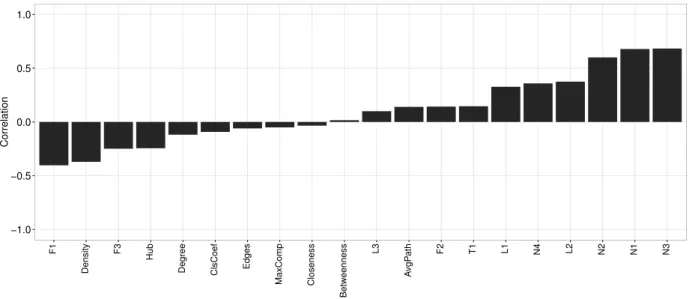
2.4 Results obtained in the Correlation Analysis . . . 27
2.4.1 Correlation of Measures with the Noise Level . . . 28
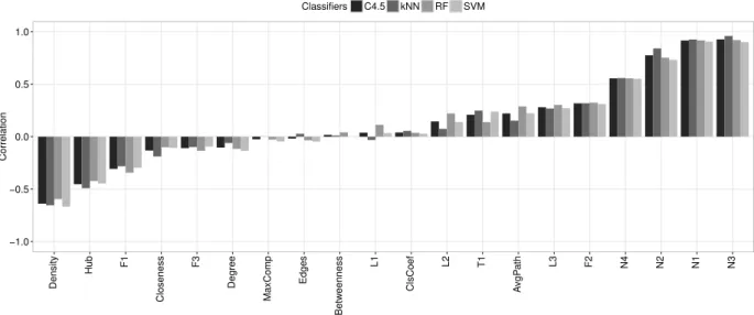
2.4.2 Correlation of Measures with the Predictive Performance . . . 29
2.4.3 Correlation Between Measures . . . 30
2.5 Chapter Remarks . . . 32
3 Noise Identification 33
3.1 Noise Filters . . . 35
3.1.1 Ensemble Based Noise Filters . . . 35
3.1.2 Noise Filters Based on Data Descriptors . . . 37
3.1.3 Distance Based Noise Filters . . . 40
3.1.4 Other Noise Filters . . . 42
3.2 Noise Filters: a Soft Decision . . . 43
3.3 Evaluation Measures for Noise Filters . . . 44
3.4 Evaluating the Noise Filters . . . 47
3.4.1 Datasets . . . 47
3.4.2 Methodology . . . 47
3.5 Experimental Evaluation of Crisp Filters . . . 49
3.5.1 Rank analysis . . . 49
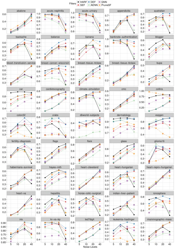
3.5.2 F1 per noise level . . . 50
3.6 Experimental Evaluation of Soft Filters . . . 54
3.6.1 Similarity and Rank analysis . . . 54
3.6.2 p@n per noise level . . . 56
3.6.3 NR-AUC per noise level . . . 61
3.7 Chapter Remarks . . . 66
4 Meta-learning 67 4.1 Modelling the Algorithm Selection Problem . . . 69
4.1.1 Instance Features . . . 70
4.1.2 Problem Instances . . . 71
4.1.3 Algorithms . . . 72
4.1.4 Evaluation measures . . . 73
4.1.5 Learning using the meta-dataset . . . 73
4.2 Evaluating MTL for NF prediction . . . 74
4.2.1 Datasets . . . 75
4.2.2 Methodology . . . 75
4.3 Experimental Evaluation to Predict the Filter Performance . . . 76
4.3.1 Experimental Analysis of the Meta-dataset . . . 76
4.3.2 Performance of the Meta-regressors . . . 77
4.4 Experimental Evaluation of the Filter Recommendation . . . 81
4.4.1 Experimental analysis of the meta-dataset . . . 81
4.4.2 Performance of the Meta-classifiers . . . 82
4.5 Case Study: Ecology Data . . . 85
4.5.1 Ecological Dataset . . . 86
4.5.3 Experimental Results . . . 87
4.6 Chapter Remarks . . . 88
5 Conclusion 91 5.1 Main Contributions . . . 92
5.2 Limitations . . . 93
5.3 Prospective work . . . 95
5.4 Publications . . . 96
List of Figures
2.1 Types of noise in classification problems. . . 11
2.2 Building a graph using ǫ-Nearest Neighbor (NN) . . . 19
2.3 Flowchart of the experiments. . . 26
2.4 Histogram of each measure for distinct noise levels. . . 28
2.5 Correlation of each measure to the noise levels. . . 29
2.6 Correlation of each measure to the predictive performance of classifiers. . . 30
2.7 Heatmap of correlation between measures. . . 31
3.1 Building the graph for an artificial dataset. . . 39
3.2 Noise detection by GNN filter. . . 41
3.3 Example of NR-AUC calculation . . . 46
3.4 Ranking of crisp NF techniques according to F1 performance. . . 49
3.5 F1 values of the crisp NF techniques per dataset and noise level. . . 51
3.6 F1 values of the crisp NF techniques per dataset and noise level. . . 52
3.7 Ranking of crisp NF techniques according to F1 performance per noise level. 53 3.8 Ranking of soft NF techniques according to p@n performance. . . 55
3.9 Dissimilarity of filters predictions. . . 56
3.10 p@n values of the best soft NF techniques per dataset and noise level. . . . 57
3.11 p@n values of the best soft NF techniques per dataset and noise level. . . . 58
3.12 Ranking of best soft NF techniques according top@nperformance per noise level. . . 60
3.13 NR-AUC values of the best soft NF techniques per dataset and noise level. 62 3.14 NR-AUC values of the best soft NF techniques per dataset and noise level. 63 3.15 Ranking of best soft NF techniques according to NR-AUC performance per noise level. . . 64
4.1 Miles (2008) algorithm selection diagram. (Adapted from Smith-Miles (2008)) . . . 70
4.2 Performance of the six crisp NF techniques. . . 78
4.3 MSE of each meta-regressor for each NF technique in the meta-dataset. . . 79
4.4 Performance of the six crisp NF techniques. . . 80
4.5 Frequency with which each meta-feature was selected by CFS technique. . 81
4.6 Distribution of highestp@n. . . 82
4.7 Accuracy of each meta-classifier in the meta-dataset. . . 83
4.8 Performance of meta-models in the base-level. . . 83
4.9 Meta DT model for NF recommendation. . . 85
List of Tables
2.1 Summary of Measures. . . 22
2.2 Summary of datasets characteristics: name, number of examples, number of features, number of classes and the percentage of the majority class. . . 25
3.1 Confusion matrix for noise detection. . . 45
3.2 Possible ensembles of NF techniques considered in this work . . . 48
3.3 Percentage of best performance for each noise level. . . 61
4.1 Summary of the characterization measures. . . 72
4.2 Summary the predictive features of the species dataset. . . 86
List of Algorithms
1 SEF . . . 36 2 Selecting m classifiers to compose the DEF ensemble . . . 37 3 Saturation Test . . . 38 4 Saturation Filter . . . 38 5 AENN . . . 42
List of Abbreviations
AENN All-k-Nearest Neighbor
ANN Artificial Neural Network
AUC Area Under the ROC Curve
CFS Correlation-based Feature Selection
CLCH Complexity of the Least Correct Hypothesis
CVCF Cross-validated Committees Filter
DCoL Data Complexity Library
DEF Dynamic Ensemble Filter
DF Default Technique
DM Data Mining
DT Decision Tree
DWNN Distance-weighted k-NN
ENN Edited Nearest Neighbor
GNN Graph Nearest Neighbor
HARF High Agreement Random Forest Filter
INFFC Iterative Noise Filter based on the Fusion of Classifiers
IPF Iterative-Partitioning Filter
IR Imbalance Ratio
ML Machine Learning
MSE Mean Squared Error
MST Minimum Spanning Tree
MTL Meta-learning
NB Naive Bayes
NDP Noisy Degree Prediction
NF Noise Filtering
NN Nearest Neighbor
NR-AUC Noise Ranking Area Under the ROC Curve
RENN Repeated Edited Nearest Neighbor
RD Random Technique
RF Random Forest
SEF Static Ensemble Filter
SF Saturation Filter
ST Saturation Test
SMOTE Synthetic Minority Over-sampling Technique
Chapter 1
Introduction
This Thesis investigates new alternatives for the use of Noise Filtering (NF) tech-niques to improve the predictive performance of classification models induced by Machine Learning (ML) algorithms.
Classification models are induced by supervised ML techniques when these techniques are applied to a labeled dataset. This Thesis will assume that a labeled dataset is com-posed bynpairs (xi, yi), where eachxi is a tuple of predictive features describing a certain
object andyi is target feature, which value corresponds to the object class. The predictive
performance of the induced model for new data depends on various factors, such as the training data quality and the inductive bias of the ML algorithm. Nonetheless, despite of the algorithm bias, when data quality is low, the performance of the predictive model is harmed.
In real world applications, there are many inconsistencies that affect data quality, such as missing data or unknown values, noise and faults in the data acquisition process (Wang et al., 1995; Fayyad et al., 1996). Data acquisition is inherently leaned to errors, even though extreme efforts are made to avoid them. It is also a resource-consuming step, since at least 60% of the efforts in a Data Mining (DM) task is spent on data preparation, which includes data preprocessing and data transformation (Pyle, 1999). Some studies estimate that, even in controlled environments, there are at least 5% of errors in a dataset (Wu, 1995; Maletic & Marcus, 2000).
Although many ML techniques have internal mechanisms to deal with noise, such as the pruning mechanism in Decision Trees (DTs) (Quinlan, 1986b,a), the presence of noise in data may lead to difficulties in the induction of ML models. These difficulties include an increase in processing time, a higher complexity of the induced model and a possible deterioration of its predictive performance for new data (Lorena & de Carvalho, 2004). When these models are used in critical environments, they may also have security and reliability problems (Strong et al., 1997).
To reduce the data modeling problems due to the presence of noise, the two usual approaches are: to employ a noise-tolerant classifier (Smith et al., 2014); or, to adopt
2 1 Introduction
a preprocessing step, also known as data cleansing (Zhu & Wu, 2004) to identify and remove noisy data. The use of noise-tolerant classifiers aims to construct robust models by using some information related to the presence of noise. The preprocessing step, on the other hand, normally involves the application of one or more NF techniques to identify the noisy data. Afterwards, the identified inconsistencies can be corrected or, more often, eliminated (Gamberger et al., 2000). The research carried out in this Thesis follows the second approach.
Even using more than one NF technique, each with a different bias, it is usually not possible to guarantee whether a given example is really a noisy example without the support of a data domain expert (Wu & Zhu, 2008; S´aez et al., 2013). Just filtering out potentially noisy data can also remove correct examples containing valuable information, which could be useful for the learning process. Thus, an extraction of noisy patterns might be needed to perform a proper filtering process. It could be done through the use of characterization measures, leading to the recommendation of the best NF using Meta-learning (MTL) for a new dataset and improves the noise detection accuracy.
The study presented in this Thesis investigates how noise affects the complexity of classification datasets identifying problem characteristics that are more sensitive to the presence of noise. This work also seeks to improve the robustness in noise detection and to recommend the best NF technique for the identification of potential noisy examples in new datasets with support of MTL. The validation of the filtering process in a real dataset is also investigated.
This chapter is structured as follows. Section 1.1 presents the main problems and gaps related to noise detection in classification tasks. Section 1.2 presents the objectives of this work and Section 1.3 defines the hypothesis investigated in this research. Finally, Section 1.4 presents the outline of this Thesis.
1.1
Motivations
The manual search for inconsistencies in a dataset by an expert is usually an unfeasible task. In the 1990s, some organizations, which used information collected from dynamic environments, spent annually, millions of dollars on training, standardization and error detection tools (Redman, 1997). In the last decades, even with the automation of the collecting processes, this cost has increased, as a consequence of the growing use of data monitoring tools (Shearer, 2000). As a result, there was an increase in data cleansing costs to avoid security and reliability problems (Strong et al., 1997).
1.1 Motivations 3
• missing values (Batista & Monard, 2003);
• outlier detection (Hodge & Austin, 2004);
• imbalanced data (Hulse et al., 2011; L´opez et al., 2013);
• noise detection (Brodley & Friedl, 1999; Verbaeten & Assche, 2003).
The noise detection is a critical component of the preprocessing step. The techniques which deal with noise in a preprocessing step are known as Noise Filtering (NF) techniques (Zhu et al., 2003). The noise detection literature commonly divides noise detection in two main approaches: noise detection in the predictive features and noise detection in the target feature.
The presence of noise is more common in the predictive features than in the target feature. Predictive feature noise is found in large quantities in many real problems (Teng, 1999; Yang et al., 2004; Hulse et al., 2007; Sahu et al., 2014). An alternative to deal with the predictive noise is the elimination of the examples where noise was detected. However, the elimination of examples with noise in predictive features could cause more harm than good (Zhu & Wu, 2004), since other predictive features from these examples may be useful to build the classifier.
Noise in the target feature is usually investigated in classification tasks, where the noise changes the true class label to another class label. A common approach to over-come the problems due to the presence of noise in the target feature is the use of NF techniques which remove potentially noisy examples. Most of the existing NF techniques focus on the elimination of examples with class label. Such approach has been shown to be advantageous (Miranda et al., 2009; Sluban et al., 2010; Garcia et al., 2012; S´aez et al., 2013; Sluban et al., 2014). Noise in the class label, from now on named class noise, can be treated as an incorrect class label value.
Several studies show that the use of these techniques can improve the classification per-formance and reduce the complexity of the induced predictive models (Brodley & Friedl, 1999; Sluban et al., 2014; Garcia et al., 2012; S´aez et al., 2016). NF techniques can rely on different types of information to detect noise, such as those employing neighborhood or density information (Wilson, 1972; Tomek, 1976; Garcia et al., 2015), descriptors extracted from the data (Gamberger et al., 1999; Sluban et al., 2014) and noise identification models induced by classifiers (Sluban et al., 2014) or ensembles of classifiers (Brodley & Friedl, 1999; Verbaeten & Assche, 2003; Sluban et al., 2010; Garcia et al., 2012). Since each NF has a bias, they can present a distinct predictive performance for different datasets (Wu & Zhu, 2008; S´aez et al., 2013). Consequently, the proper management of NF bias is expected to lead to an improvement on the noise detection accuracy.
4 1 Introduction
classification dataset can be used to detect the presence or absence of noise in the dataset. These measures can be used to assess the complexity of the classification task (Ho & Basu, 2002; Orriols-Puig et al., 2010; Kolaczyk, 2009). For such, they take into account the overlap between classes imposed by feature values, the separability and distribution of the data points and the value of structural measures based on the representation of the dataset as a graph structure. Accordingly, experimental results show that the addition of noise in a dataset affects the geometry of the classes separation, which can be captured by these measures (S´aez et al., 2013).
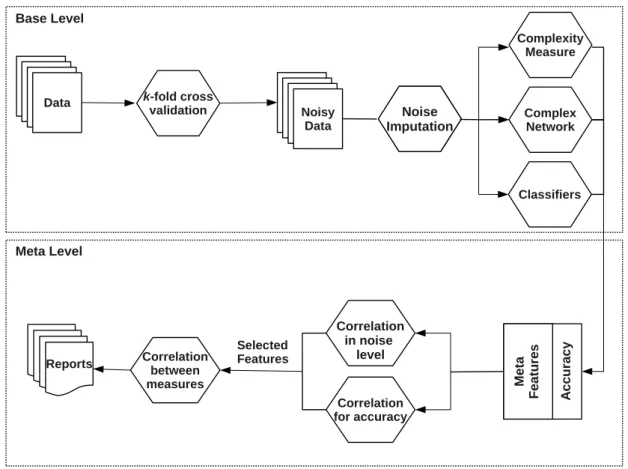
Another open research issue is the definition of how suitable a NF technique is for each dataset. MTL has been largely used in the last years to support the recommendation of the most suitable ML algorithm(s) for a new dataset (Brazdil et al., 2009). Given a set of widely used NF techniques and a set of complexity measures able to characterize datasets, an automatic system could be employed to support the choice of the most suitable NF technique by non-experts. In this Thesis, we investigate the support provided by the proposed MTL-based recommendation system. The experiments were based on a meta-dataset consisting of complexity measures extracted from a collection of several artificially corrupted datasets along with information about the performance of widely used NF techniques.
1.2
Objectives and Proposals
The main goal of this study is the investigation of class label noise detection in a preprocessing step, providing new approaches able to improve the noise detection predic-tive performance. The proposed approaches include the study of the use of complexity measures to identify noisy patterns, the development of new techniques to fill gaps in ex-isting techniques regarding predictive performance in noise detection and the use of MTL to recommend the most suitable NF technique(s). Another contribution of this study is the validation of the proposed approaches on a real dataset with an application domain expert.
1.2 Objectives and Proposals 5
be applied whether a new dataset should be cleaned by a NF technique.
Even for the well-known NF techniques that use different types of information to detect noise, such as neighborhood or density information, descriptors extracted from the data and noise identification models induced by classifiers or ensembles of classifiers, there is usually a margin of improvement on the noise detection accuracy. Two NF techniques are proposed, one of them based on a subset of complexity measures capable to detect noisy patterns and the other based on a committee of classifiers - both can increase the robustness in the noise identification.
Most NF techniques adopt a crisp decision for noise identification, classifying each training example as either noisy or safe. Soft decision strategies, on the other hand, assign a Noisy Degree Prediction (NDP) to each example. In practice, this allows not only to identify, but also to rank the potential noisy cases, evidencing the most unreliable instances. These examples could then be further examined by a domain expert. The adaptation of the original NF techniques for soft decision and the aggregation of differ-ent individual techniques can improve noise detection accuracy. These issues are also investigated in this Thesis.
The bias of each NF technique influences its predictive performance on a particular dataset. Therefore, there is no single technique that can be considered the best for all domains or data distributions and choosing a particular filter for a new dataset is not straightforward. An alternative to deal with this problem is to have a model able to recommend the best NF technique(s) for a new dataset. MTL has been successfully used for the recommendation of the most suitable technique for each one of several tasks, like classification, clustering, time series analysis and optimization. Thus, MTL would be a promising approach to induce a model able to predict the performance and recommend the best NF techniques for a new dataset. Its use could reduce the uncertainty in the selection of NF technique(s) and improve the label noise identification.
The predictive accuracy of MTL depends on how a dataset is characterized by features. Thus, the first step to use MTL is to create a dataset, with one meta-example representing each dataset. In this meta-dataset, for each meta-meta-example, the predictive features are the meta-features extracted from a dataset and the target feature is the technique(s) with the best performance in the dataset.
The set of meta-features used in this Thesis describes various characteristics for each dataset, including its expected complexity level (Ho & Basu, 2002). Examples in this meta-dataset are labeled with the performance achieved by the NF technique in the noise identification. ML techniques from different paradigms are applied to the meta-dataset to induce a meta-model, which is used in a recommendation system to predict the best NF technique(s) for a new dataset.
6 1 Introduction
is analyzed by a domain expert. The dataset used for this validation shows the presence or absence of species in georeferenced points. Both classes present label noise: the absence of the species can be a misclassification if the point analyzed does not represent the protected area or even the false presence if the point analyzed does not have environmental compatibility in a long-term window.
All experiments use a large set of artificial and public domain datasets like UCI1 with different levels of artificial imputed noise (Lichman, 2013). The NF evaluation is per-formed by standard measures, which are able to quantify the quality of the preprocessed datasets. The quality is related to the noisy cases correctly identified among those exam-ples identified as noisy by the filter and noisy cases correctly identified among the noisy cases present in the dataset.
1.3
Hypothesis
Considering the current limitations and the existence of margins for improvement in noise detection in classification datasets, this work investigated four main hypotheses aiming to make inferences about the impact of label noise in classification problems and the possibility to performing data cleansing effectively. The hypotheses are:
1. The characterization of datasets by complexity and structural measures
can help to better detect noisy patterns. Noise presence may affect the com-plexity of the classification problem, making it more difficult. Thereby, monitoring several measures in the presence of different label noise levels can indicate the mea-sures that are more sensitive to the presence of label noise, and can thereby be used to support noise identification. Geometric, statistical and structural measures are extracted to characterize the complexity of a classification dataset.
2. New techniques can improve the state of the art in noise detection. Even
with a high number of NF techniques, there is no single technique that has satisfac-tory results for all different niches and different noise levels. Thus, new techniques for NF can be investigated. The proposed NF techniques are based on a subset of complexity measures able to detect noisy patterns and based on an ensemble of classifiers.
3. Noise filters techniques can be adapted to provide a NDP, which can
increase the data understanding and the noise detection accuracy. In
order to highlight the most unreliable instances to be further examined, the rank of the potential noisy cases can increase the data understanding and it even makes easier to combine multiple filters in ensembles. While the expert can use the rank
1.4 Outline 7
of unreliable instances to understand the noisy patterns, the ensembles can combine the NF techniques to increase the noise detection accuracy for a larger number of datasets than the individual techniques used alone.
4. A model induced using meta-learning can predict the performance or
even recommend the best NF technique(s) for a new dataset. The bias of
each NF technique influences its predictive performance on a particular dataset. Therefore, there is no single technique that can be considered the best for all datasets. A MTL system able to predict the expected performance of NF tech-niques in noisy data identification tasks could recommend the most suitable NF technique(s) for a new dataset.
1.4
Outline
The remainder of this Thesis is organized as follows:
Chapter 2 presents an overview of noisy data and complexity measures that can be used to characterize the complexity of noisy classification datasets. Preliminary experiments are performed to analyse the measures and, based on the experimental results, a subset of measures is suggested as more sensitive to the addition of noise in a dataset.
Chapter 3 addresses the preprocessing step, describing the main NF techniques. This chapter also proposed two new NF, one of them based in the experimental results presented in the previous chapter and the other based on the use of an ensemble of classifiers. In this chapter the NF techniques are also adapted to rank the potential noisy cases to increase the data understanding. Experiments are performed to analyse the predictive performance of the NF techniques for different noise levels with different evaluation measures.
Chapter 4 focuses on MTL, explaining the main meta-features and the algorithm selection problem adopted in this research. Experiments using MTL for NF technique recommendation are carried out, to predict the NF technique predictive performance and to recommend the best NF technique. In this chapter, a validation of the recommendation system approach on a real dataset with support of a domain expert is also presented.
Chapter 2
Noise in Classification Problems
The characterization of a dataset by the amount of information present in the data is a difficult task (Hickey, 1996). In many cases, only an expert can analyze the dataset and provide an overview about the dispersion concepts and the quality of the information present in the data (Pyle, 1999). Dispersion concepts are those associated with the process of identifying, understanding and planning the information to be collected, while quality of the information is related with the addition of inconsistencies in the collection process. Since the analysis of dispersion concepts is very difficult, it is natural to consider only the aspects associated with inconsistencies.
These inconsistencies can be absent of information (missing or unknown values), noise or errors (Wang et al., 1995; Fayyad et al., 1996). Even with extreme efforts to avoid noise, it is very difficult to ensure a data acquisition process without errors. Whereas the noise data needs to be identified and treated, secure data must be preserved in the dataset (Sluban et al., 2014). The term secure data usually refers to instances that are the core of the knowledge necessary to build accurate learning models (Quinlan, 1986b). This study deals with the problem of identifying noise in labeled datasets.
Various strategies and techniques have been proposed in the literature to reduce the problems derived from the presence of noisy data (Tomek, 1976; Brodley & Friedl, 1996; Verbaeten & Assche, 2003; Sluban et al., 2010; Garcia et al., 2012; Sluban et al., 2014; Smith et al., 2014). Some recent proposals include designing classification techniques more tolerant and robust to noise, as surveyed in Frenay & Verleysen (2014). Generally, the data identified as noisy are first filtered and removed from the datasets. Nonetheless, it is usually difficult to determine if a given instance is indeed noisy or not.
Despite the strategy employed to deal with noisy data, either by data cleansing or by the design of noise-tolerant learning algorithms, it is important to understand the effects that the presence of noise in a dataset cause in classification tasks. The use of measures capable to characterize the presence or absence of noise in a dataset could assist the noise detection or even the decision of whether a new dataset needs to be cleaned by a NF technique. Complexity measures may play an important role in this issue. A
10 2 Noise in Classification Problems
recent work that uses complexity measures in the NF scenario is S´aez et al. (2013). The authors employ these measures to predict whether a NF technique is effective for cleaning a dataset that will be used for the induction of k-NN classifiers.
The approach presented in S´aez et al. (2013) differs from the approach proposed in this Thesis in several aspects. One of the main differences is that, while the approach proposed by S´aez et al. (2013) is restricted to k-NN classifiers, the proposed approach investigates how noise affects the complexity of the decision border that separates the classes. For such, it employs a series of statistic and geometric measures originally described in Ho & Basu (2002). These measures evaluate the difficulty of a classification task of a given dataset by analyzing some characteristics of the dataset and the predictive performance of some simple classification models induced from this dataset. Furthermore, the proposed approach uses new measures able to represent a dataset through a graph structure, named here structural measures (Kolaczyk, 2009; Morais & Prati, 2013).
The studies presented in this Thesis allow a better understanding of the effects of noise in the predictive performance of predictive models in classification tasks. Besides, they allow the identification of problem characteristics that are more sensitive to the presence of noise and that can be further explored in the design of new noise handling techniques. To make the reading of this text more direct, from now on, this Thesis will refer to complexity of datasets associated with classification tasks as complexity of classification tasks.
The main contributions from this chapter can be summarized as:
• Proposal of a methodology for the empirical evaluation of the effects of different levels of label noise in the complexity of classification datasets;
• Analysis of the sensibility of various measures associated with the geometrical com-plexity of classification datasets to detect the presence of label noise;
• Proposal of new measures able to evaluate the structural complexity of a classifica-tion dataset;
• Highlight complexity measures that can be further explored in the proposal of new noise handling techniques.
2.1 Types of Noise 11
2.1
Types of Noise
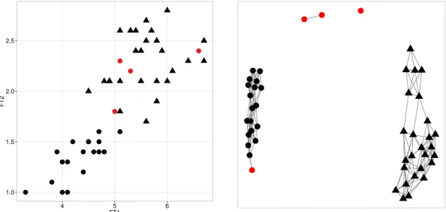
Noisy data also can be regarded as objects that present inconsistencies in their pre-dictive and/or target feature values (Quinlan, 1986a). For supervised learning datasets, Zhu & Wu (2004) distinguish two types of noise: (i) in the predictive features and (ii) in the target feature. Noise in predictive features is introduced in one or more predictive features as consequence of incorrect, absent or unknown values. On the other hand, noise in target features occurs in the class labels. They can be caused by errors or subjectivity in data labeling, as well as by the use of inadequate information in the labeling process. Lately, noise in predictive features can lead to a wrong labeling of the data points, since they can be moved to the wrong side of the decision border.
The artificial binary dataset shown in Figure 2.1 illustrates these cases. The original dataset has 2 classes (•and N) that are linearly separable. Figure 2.1(a) shows the same artificial dataset with two potential predictive noisy examples, while Figure 2.1(b) has two potential label noisy examples. Although the noise identification for this artificial dataset is rather simplistic, for instance when the degree of noise in the predictive features is lower, the noise detection capability can dramatically decrease.
1.2 1.5 1.8 2.1
2.5 3.0 3.5 4.0 4.5 5.0
FT1
FT2
(a) Noise in predictive feature
1.2 1.5 1.8 2.1
2.5 3.0 3.5 4.0 4.5 5.0
FT1
FT2
(b) Noise in target feature
Figure 2.1: Types of noise in classification problems.
12 2 Noise in Classification Problems
noise will refer to label noise.
Ideally, noise identification should involve a validation step, where the objects high-lighted as noisy are confirmed as such, before they can be further processed. Since the most common approach is to eliminate noisy data, it is important to properly distinguish these data from the safe data. Safe data need to be preserved, once they have features that represent part of the knowledge necessary for the induction of an adequate model.
In a real application, evaluating whether a given example is noisy or not usually has to rely on the judgment of a domain specialist, which is not always available. Furthermore, the need to consult a specialist tends to increase the cost and duration of the preprocessing step. This problem is reduced when artificial datasets are used, or when simulated noise is added to a dataset in a controlled way. The systematic addition of noise simplifies the validation of the noise detection techniques and the study of noise influence in the learning process.
There are two main methods to add noise to the class feature: (i) random, in which each example has the same probability of having its label corrupted (exchanged by another label) (Teng, 1999); and (ii) pairwise, in which a percentage x% of the majority class examples have their labels modified to the same label of the second majority class (Zhu et al., 2003). Whatever the strategy employed to add noise to a dataset, it is necessary to corrupt the examples within a given rate. In most of the related studies, noise is added according to rates that range from 5% to 40%, with intervals of 5% (Zhu & Wu, 2004), although other papers opt for fixed rates (as 2%, 5% and 10%) (Sluban et al., 2014). Besides, due to its stochastic nature, this addition is normally repeated a number of times for each noise level.
2.2
Describing Noisy Datasets: Complexity Measures
Each noise-tolerant technique and cleansing filter has a distinct bias when dealing with noise. To better understand their particularities, it is important to know how noisy data affects a classification problem. According to Li & Abu-Mostafa (2006), noisy data tends to increase the complexity of the classification problem. Therefore, the identification and removal of noise can simplify the geometry of the separation border between the problem classes (Ho, 2008).
2.2 Describing Noisy Datasets: Complexity Measures 13
a modification of the error function minimized during neural networks training, so that hard instances have a lower weight on the error function update. The second proposal is a NF technique that removes hard instances, which correspond to potential noisy data. All previous work confirm the effect of noise in the complexity of the classification problem.
This work evaluates deeply the effects of different noise levels in the complexity of the classification problems, by extracting different measures from the datasets and monitoring their sensitivity to noise imputation. According to Ho & Basu (2002), the difficulty of a classification problem can be attributed to three main aspects: the ambiguity among the classes, the complexity of the separation between the classes, and the data sparsity and dimensionality. Usually, there is a combination of these aspects. They propose a set of geometrical and statistical descriptors able to characterize the complexity of the classi-fication problem associated with a dataset. Originally proposed for binary classiclassi-fication problems (Ho & Basu, 2002), some of these measures were later extended to multiclass classification in Mollineda et al. (2005); Lorena & de Souto (2015) and Orriols-Puig et al. (2010). For measures only suitable for binary classification problems, we first transform the multiclass problem into a set of binary classification subproblems by using the one-vs-all approach. The mean of the complexity values obtained in such subproblems is then used as an overall measure for the multiclass dataset.
The descriptors of Ho & Basu (2002) can be divided into three categories:
Measures of overlapping in the feature values. Assess the separability of the classes in a dataset according to its predictive features. The discriminant power of each feature reflects its ambiguity level compared to the other features.
Measures of class separability. Quantify the complexity of the decision boundaries separating the classes. They are usually based on linearity assumptions and on the distance between examples.
Measures of geometry and topology. They extract features from the local
(geome-try) and global (topology) structure of the data to describe the separation between classes and data distribution.
Additionally, a classification dataset can be characterized as a graph, allowing the extraction of some structural measures from the data. Modeling a classification dataset through a graph allows capturing additional topological and structural information from a dataset. In fact, graphs are powerful tools for representing the information of relations between data (Ganguly et al., 2009). Therefore, this work includes an additional class of complexity measures in the experiments related to noise understanding:
Measures of structural representation. They are extracted from a structural
14 2 Noise in Classification Problems
The recent work of Smith et al. (2014) also proposes a new set of measures, which are intended to understand why some instances are hard to classify. Since this type of analysis is not within the scope of this thesis, these measures were not included in the experiments.
2.2.1
Measures of Overlapping in Feature Values
Fisher’s discriminant ratio (F1): Selects the feature that best discriminates the classes. It can be calculated by Equation 2.1, for binary classification problems, and by Equation 2.2 for problems with more than two classes (C classes). In these equations,m is the number of input features and fi is the i-th predictive feature.
F1 = maxm
i=1 (µfi
c1 −µ
fi
c2)
2
(σfi
c1)2+ (σ
fi
c2)2
(2.1)
F1 =maxm
i=1
PC
cj=1
PC
ck=cj+1pcjpck(µ
fi
cj −µ
fi
ck)
2
PC
cj=1pcjσ
2
cj
(2.2)
For continuous features, µfi
cj and (σ
fi
cj)
2 are, respectively, the average and standard
deviation of the feature fi within the class cj. Nominal features are first mapped
into numerical values and µfi
cj is their median value, while (σ
fi
cj)
2 is the variance
of a binomial distribution, as presented in Equation 2.3, where pµfi
cj is the median
frequency andncj is the number of examples in the class cj. σfi
cj =
q
pµfi
cj(1−pµficj)∗ncj (2.3)
High values of F1 indicate that at least one of the features in the dataset is able to linearly separate data from different classes. Low values, on the other hand, do not indicate that the problem is non-linear, but that there is not an hyperplane orthogonal to one of the data axis that separates the classes.
Directional-vector maximum Fisher’s discriminant ratio (F1v): this measure
complements F1, modifying the orthogonal axis in order to improve data projection. Equation 2.4 illustrates this modification.
R(d) = d
T(µ
1−µ2)(µ1 −µ2)Td
dTΣ¯d (2.4)
Where:
• dis the directional vector where data are projected, calculated asd= ¯Σ−1(µ 1−
2.2 Describing Noisy Datasets: Complexity Measures 15
• µi is the mean feature vector for the class ci;
• Σ =¯ αΣ1+ (1−α)Σ2,0≤α≤1;
• Σi is the covariance matrix for the examples from the class ci.
This measure can be calculated only for binary classification problems. A high F1v value indicates that there is a vector that separates the examples from distinct classes, after they are projected into a transformed space.
Overlapping of the per-class bounding boxes (F2): This measure calculates the
volume of the overlapping region on the feature values for a pair of classes. This overlapping considers the minimum and maximum values of each feature per class in the dataset. A product of the calculated values for each feature is generated. Equation 2.5 illustrates F2 as it is defined in (Orriols-Puig et al., 2010), where fi is
the feature iand c1 and c2 are two classes.
F2 =
m
Y
i=1
|min(max(fi, c1), max(fi, c2))−max(min(fi, c1), min(fi, c2))
max(max(fi, c1), max(fi, c2))−min(min(fi, c1), min(fi, c2))
| (2.5)
In multiclass problems, the final result is the sum of the values calculated for the underlying binary subproblems. A low F2 value indicates that the features can discriminate the examples of distinct classes and have low overlapping.
Maximum individual feature efficiency (F3): Evaluates the individual efficacy of each feature by considering how much each feature contributes to the classes sepa-ration. This measure uses examples that are not in overlapping ranges and outputs an efficiency ratio of linear separability. Equation 2.6 shows how F3 is calculated, wheren is the number of examples in the training set andoverlapis a function that returns the number of overlapping examples between two classes. High values of F3 indicate the presence of features whose values do not overlap between classes.
F3 =maxm
i=1
n−overlap(xfi
c1,x
fi
c2)
n (2.6)
Collective feature efficiency (F4): based on F3, this measure evaluates the collective power of discrimination of the features. It uses an iterative procedure selecting the feature with the highest discrimination power and removing these examples from the dataset. The procedure is repeated until all examples are discriminated or all features are analysed, returning the proportion of instances that have been discriminated. Equation 2.7 shows how F4 is calculated, where overlap(xfi
c1,x
fi
16 2 Noise in Classification Problems
measure the overlap in a subset of the dataTi generated by removing the examples
already discriminated inTi−1.
F4 =
m
X
i=1
overlap(xfi
c1,x
fi
c2)Ti
n (2.7)
Higher values indicate that more examples can be discriminated by using a combi-nation of the available features.
2.2.2
Measures of Class Separability
Distance of erroneous instances to a linear classifier(L1): This measure quantifies the linearity of data, since the classification of linear separable data is considered a simpler classification task. L1 computes the sum of the distances of erroneous data to an hyperplane separating two classes. Support Vector Machine (SVM) with a linear kernel function (Vapnik, 1995) are used to induce the hyperplane. This measure is used only for binary classification problems. In Equation 2.8, f(·) is the linear function, h(·) is the prediction and yi is the class of xi. Values equal to 0
indicate a linearly separable problem.
L1 = X
h(xi)6=yi
f(xi) (2.8)
Training error of a linear classifier (L2): Measures the predictive performance of a linear classifier for the training data. It also uses a SVM with linear kernel. Equation 2.9 shows how L2 is calculated. The h(xi) is the prediction of the linear
classifier obtained and I(·) is the evalaution measure which returns 1 if xi is true
and 0 otherwise. A lower training error indicate the linearity of the problem.
L2 =
Pn
i=1I(h(xi)6=yi)
n (2.9)
Fraction of points lying on the class boundary (N1): Estimates the
complex-ity of the correct hypothesis underlying the data. Initially, a Minimum Spanning Tree (MST) is generated from the data, connecting the data points by their dis-tances. The fraction of points from different classes that are connected in the MST is returned. Equation 2.10 defines how N1 is calculated. The xj ∈N N(xi) verify if
xj is the NN example andyi 6=yj verify if they are examples of different class. High
values of N1 indicate the need for more complex boundaries for separating the data.
N1 =
Pn
i=1I(xj ∈N N(xi) and yi 6=yj)
2.2 Describing Noisy Datasets: Complexity Measures 17
Average intra/inter class nearest neighbor distances (N2): The mean
intra-class and inter-intra-class distances use the k-Nearest Neighbor (k-NN) (Mitchell, 1997) algorithm to analyse the spread of the examples from distinct classes. The intra-class distance considers the distance from each example to its nearest example in the same class, while the inter-class distance computes the distance of this example to its nearest example in other class. Equation 2.11 illustrates N2, where intra and inter are distance function.
N2 =
Pn
i=1intra(xi)
Pn
i=1inter(xi)
(2.11)
Low N2 values indicate that examples of the same class are next to each other, while far from the examples of the other classes.
Leave-one-out error rate of the 1-NN algorithm (N3): Evaluates how distinct
the examples from different classes are by considering the error rate of the 1-NN (Mitchell, 1997) classifier, with the leave-one-out strategy. Equation 2.12 shows the N3 measure. Low values indicate a high separation of the classes.
N3 =
Pn
i=1I(1N N(xi)6=yi)
n (2.12)
2.2.3
Measures of Geometry and Topology
Nonlinearity of a linear classifier (L3): Creates a new dataset by the interpolation of training data. New examples are created by linear interpolation with random coefficients of points chosen from a same class. Next, a SVM (Vapnik, 1995) classifier with linear kernel function is induced and its error rate for the original data is recorded. It is sensitive to the spread and overlapping of the data points and is used for binary classification problems only. Equation 2.13 illustrate the L3 measure, where l is the number of points and the examples generated by the interpolation. Low values indicate a high linearity.
L3 =
Pl
i=1I(h(xi)6=yi)
l (2.13)
Nonlinearity of the 1-NN classifier (N4): Has the same reasoning of L3, but us-ing the 1-NN (Mitchell, 1997) classifier instead of the linear SVM (Vapnik, 1995). Equation 2.14 illustrate the N4 measure.
N4 =
Pl
i=1I(1N N(xi)6=yi)
18 2 Noise in Classification Problems
Fraction of maximum covering spheres on data (T1): Builds hyperspheres
cen-tered on the data points. The radius of these hyperspheres are increased until touching any example of different classes. Smaller hyperspheres inside larger ones are eliminated. It outputs the ratio of the number of hyperspheres formed to the to-tal number of data points. Equation 2.15 shows T1, wherehyperpheres(D) returns the number of hyperspheres which can be built from the dataset. Low values indicate a low number of hyperspheres due to a low complexity of the data representation.
T1 = hyperpheres(D)
n (2.15)
There are other measures presented in Ho & Basu (2002) and Orriols-Puig et al. (2010) that were not employed in this work because, by definition, they do not vary when the label noise level is increased. One of them is the dimensionality of the dataset and another is the ratio of the number of features to the number of data points (data sparsity).
2.2.4
Measures of Structural Representation
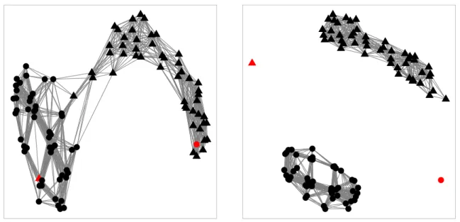
Before using these measures, it is necessary to transform the classification dataset into a graph. This graph must preserve the similarities and distances between examples, so that the data relationships are captured. Each data point will correspond to a node or vertex of the graph. Edges are added connecting all pairs of nodes or some of the pairs.
Several techniques can be used to build a graph for a dataset. The most common are the k-NN and the ǫ-NN (Zhu et al., 2005). While k-NN connects a pair of vertices i and j whenever i is one of the k-NN of j, ǫ-NN connects a pair of nodes i and j only if d(i, j) < ǫ, where d is a distance function. We employed the ǫ-NN variant, since many edge and degree based measures could be fixed fork-NN, despite the level of noise inserted in a dataset. Afterwards, all edges between examples from different classes are pruned from the graph (Zhu et al., 2005). This is a postprocessing step that can be employed for labeled datasets, which takes into account the class information.
2.2 Describing Noisy Datasets: Complexity Measures 19 ● ● ● ● ● ● ● ● ● ● ● ● ● ● ● ● ● ● ● ● ● ● ● ● ● ● ● ● ● ● ● ● ● ● ● ● ● ● ● ● ● ● ● ● ● ● ● ● ● ●
(a) Building the graph (unsupervised)
● ● ● ● ● ● ● ● ● ● ● ● ● ● ● ● ● ● ● ● ● ● ● ● ● ● ● ● ●● ● ● ● ● ● ● ● ● ● ●● ● ● ● ● ● ● ● ● ●
(b) Pruning process (supervised)
Figure 2.2: Building a graph using ǫ-NN
Number of edges (Edges): Total number of edges contained in the graph. High
values for edge-related measures indicate that many of the vertices are connected and, therefore, that there are many regions of high densities from a same class. This is true because of the postprocessing of edges connecting examples from different classes applied in this work. Equation 2.16 illustrate the measure, wherevij is equal
to 1 if i and j are connected, and 0 otherwise. Thus, the dataset is regarded as having low complexity if it shows a high number of edges.
edges=X
i,j
vij (2.16)
Average degree of the network (Degree): The degree of a vertex i is the number of edges connected to i. The average degree of a network is the average degree of all vertices in the graph. For undirected networks, it can be computed by Equation 2.17.
degree= 1 n
X
i,j
vij (2.17)
The same reasoning of edge-related measures applies to degree based measures, since the degree of a vertex corresponds to the number of edges incident to it. Therefore, high values for the degree indicates the presence of many regions of high densities from a same class, and the dataset can be regarded as having low complexity.
20 2 Noise in Classification Problems
number of edges it contains by the number of possible edges that could be formed. The average density also allows capturing whether there are dense regions from the same class in the dataset. Equation 2.18 illustrate the measure, where n is the number of vertices and n(n2−1) is the number of possible edges. High values indicate the presence of such regions and a simpler dataset.
density = 2 n(n−1)
X
i,j
vij (2.18)
Maximum number of components(MaxComp): Corresponds to the maximal
num-ber of connected components of a graph. In an undirected graph, a component is a subgraph with paths between all of its nodes. When a dataset shows a high overlap-ping between classes, the graph will probably present a large number of disconnected components, since connections between different classes are pruned from the graph. The minimal component will tend to be smaller in this case. Thus, we will assume that smaller values of the MaxComp measures represent more complex datasets.
Closeness centrality (Closeness): Average number of steps required to access every other vertex from a given vertex, which is the number of edges traversed in the shortest path between them. It can be computed by the inverse of the distance between the nodes, as shown in Equation 2.19:
closeness= P 1
i6=jd(vij)
(2.19)
Since the closeness measure uses the inverse of the shortest distance between vertices, larger values are expected for simpler datasets that will show low distances between examples from the same class.
Betweenness centrality (Betweenness): The vertex and edge betweenness are
de-fined by the average number of shortest paths that traverses them. We employed the vertex variant. Equation 2.20 represents the betweenness value of a vertex vj,
where d(vil) is the total number of the shortest paths from node i to node l and
dj(vil) is the number of those paths that pass throughj:
betweenness(vj) =
X
i6=j6=l
dj(vil)
d(vil)
(2.20)
The value of Betweenness will be small for simpler datasets, since the distance between the shortest paths and the paths which pass through j will be close.
2.2 Describing Noisy Datasets: Complexity Measures 21
ratio of the number of edges between its neighbors (ki) and the maximum number of
edges that could possibly exist between these neighbors. Equation 2.21 illustrate this measure. Measure ClsCoef will be higher for simpler datasets, which will produce large connected components joining vertices from the same class.
ClsCoef(vi) =
2 ki(ki−1)
X
i,j∈k
vij (2.21)
Hub score (Hubs): Measures the score of each node by the number of connections it has to other nodes, weighted by the number of connections these neighbors have. That is, more connected vertices, which are also connected to highly connected vertices, have higher hub score. The hub score is expected to have a low mean for high complexity datasets, since strong vertices will become less connected to strong neighbors. For instance, hubs are expected at regions of high density from a given class. Therefore, simpler datasets with high density will show larger values for this measure.
Average Path Length (AvgPath): Average size of all shortest paths in the graph. It measures the efficiency of information spread in the network. It is illustrated by Equation 2.22, where n represents the number of vertices of the graph andd(vij) is
the shortest distance between vertices iand j.
AvgP ath= 2 n(n−1)
X
i6=j
d(vij); (2.22)
For the AvgPath measure, high values are expected for low density graphs, indicating an increase in complexity.
For those measures that are calculated for each vertex individually, we computed an average for all vertices in the graph. The graph measures used in this study mainly evaluate the overlapping of the classes and their density.
22 2 Noise in Classification Problems
average clustering coefficient and the average degree. Besides introducing new measures, we also describe the behavior of all measures for simpler or complex problems. Moreover, we try to identify the best suited measures for detecting the presence of label noise in a dataset.
2.2.5
Summary of Measures
Table 2.1 summarizes the measures employed to characterize the complexity of the datasets used in this study. For each measure, we present upper (Maximum value) and lower bounds (Minimum value) achievable and how they are associated with the increase or decrease of complexity of the classification problems (Complexity column). For a given measure, the value in column “Complexity” is “+” if higher values of the measure are observed for high complexity datasets, that is, when the measure value correlates positively to the complexity level. On the other hand, the “-” sign denotes the opposite, so that low values of the measure are obtained for high complexity datasets, denoting a negative correlation.
Table 2.1: Summary of Measures.
Type of Measure Measure Minimum Value Maximum Value Complexity
Overlapping in feature values
F1 0 +∞
-F1v 0 +∞
-F2 0 +∞ +
F3 0 1
-F4 0 +∞
-Class separability
L1 0 +∞ +
L2 0 1 +
N1 0 1 +
N2 0 +∞ +
N3 0 1 +
Geometry and topology
L3 0 1 +
N4 0 1 +
T1 0 1 +
Structural representation
Edges 0 n∗(n−1)/2
-Degree 0 n−1
-MaxComp 1 n
-Closeness 0 1/(n−1)
-Betweenness 0 (n−1)∗(n−2)/2 +
Hubs 0 1
-Density 0 1
-ClsCoef 0 1
-AvgPath 1/n∗(n−1) 0.5 +
2.3 Evaluating the Complexity of Noisy Datasets 23
We denote that by the “∞” value in the Table 2.1. In the case of graph-based measures, we
generated graphs representing simple and complex relations between the same number of data points and observed the achieved measure values. A simple graph would correspond to a case where the classes are well separated and there is a high number of connections between examples from the same class, while a complex dataset would correspond to a graph where examples of different classes are always next to each other and ultimately the connections between them are pruned according to our graph construction method.
2.3
Evaluating the Complexity of Noisy Datasets
This section presents the experiments performed to evaluate how the different data complexity measures from Section 2.2 behave in the presence of label noise for several benchmark public datasets. First, a set of classification benchmark datasets were chosen for the experiments. Different levels of label noise were later added to each dataset. The experiments also monitor how the complexity level of the datasets are affected by noise imputation. This is accomplished by:
1. Verifying the Spearman correlation between the measure values with the noise rates artificially imputed and the predictive performance of a group of classifiers. This analysis allows the identification of a set of measures that are more sensitive to the presence of noise in a dataset.
2. Evaluating the correlation between the measure values in order to identify those measures that (i) capture different concepts regarding noisy environments and (ii) can be jointly used to support the development of new noise-handling techniques.
The next sections present in detail the experimental protocol previously outlined.
2.3.1
Datasets
24 2 Noise in Classification Problems
Regarding the real datasets, 90 benchmarks were selected from the UCI1 repository (Lichman, 2013). Because they are real, it is not possible to assert that they are noise-free, although some of them are artificial and show no label inconsistencies. Nonetheless, a recent study showed that most of the datasets from UCI can be considered easy prob-lems, once many classification techniques are able to obtain high predictive accuracies when applied to them (Maci´a & Bernad´o-Mansilla, 2014). Table 2.2 summarizes the main characteristics of the datasets used in the experiments of this Thesis: number of exam-ples (#EX), number of features (#FT), number of classes (#CL) and percentage of the examples in the majority class (%MC).
In order to corrupt the datasets with noise, the uniform random addition method, which is the most common type of artificial noise imputation method for classification tasks (Zhu & Wu, 2004), was used. For each dataset, noise was inserted at different levels, namely 5%, 10%, 20% and 40%. Thus, making possible to investigate the influence of increasing noise levels in the results. Besides, all datasets were partitioned according to 10-fold-cross-validation, but noise was inserted only in the training folds. Once the selection of examples was random, 10 different noisy versions of the training data for each noise level were generated.
2.3.2
Methodology
Figure 2.3 shows the flow chart of the experimental methodology. First, noisy versions of the original datasets from Section 2.3.1 were created by using the previously described systematic model of noise imputation. The complexity measures and the predictive per-formance of classifiers were extracted from the original training datasets and from their noisy versions.
To calculate the complexity measures described from Section 2.2.1 to Section 2.2.3, the Data Complexity Library (DCoL) (Orriols-Puig et al., 2010) was used. All distance-based measures employed the normalized euclidean distance for continuous features and the overlap distance for nominal features (this distance is 0 for equal categorical values and 1 otherwise) (Giraud-Carrier & Martinez, 1995). To build the graph for the graph-based measures, the ǫ-NN algorithm, with theǫ threshold value equal to 15%, was used, like in Morais & Prati (2013). The measures described in Section 2.2.4 were calculated using the Igraph library (Csardi & Nepusz, 2006). Measures like the directional-vector Fisher’s discriminant ratio (F1v) and collective feature efficiency (F4) from Orriols-Puig et al. (2010) were disregarded in this particular analysis, since they have a concept similar to other measures already employed.
The application of these measures result in one meta-dataset, which will be employed in the subsequent experiments. This meta-dataset contains 20 meta-features (# complexity
2.3 Evaluating the Complexity of Noisy Datasets 25
Table 2.2: Summary of datasets characteristics: name, number of examples, number of features, number of classes and the percentage of the majority class.
Dataset #EX #FT #CL %MC Dataset #EX #FT #CL %MC
abalone 4153 9 19 17 meta-data 528 22 24 4
acute-nephritis 120 7 2 58 mines-vs-rocks 208 61 2 53
acute-urinary 120 7 2 51 molecular-promoters 106 58 2 50
appendicitis 106 8 2 80 molecular-promotor 106 58 2 50
australian 690 15 2 56 monks1 556 7 2 50
backache 180 32 2 86 monks2 601 7 2 66
balance 625 5 3 46 monks3 554 7 2 52
banana 5300 3 2 55 movement-libras 360 91 15 7
banknote-authentication 1372 5 2 56 newthyroid 215 6 3 70
blogger 100 6 2 68 page-blocks 5473 11 5 90
blood-transfusion-service 748 5 2 76 parkinsons 195 23 2 75
breast-cancer-wisconsin 699 10 2 66 phoneme 5404 6 2 71
breast-tissue-4class 106 10 4 46 pima 768 9 2 65
breast-tissue-6class 106 10 6 21 planning-relax 182 13 2 71
bupa 345 7 2 58 qualitative-bankruptcy 250 7 2 57
car 1728 7 4 70 ringnorm 7400 21 2 50
cardiotocography 2126 21 10 27 saheart 462 10 2 65
climate-simulation 540 21 2 91 seeds 210 8 3 33
cmc 1473 10 3 43 segmentation 2310 19 7 14
collins 485 22 13 16 spectf 349 45 2 73
colon32 62 33 2 65 spectf-heart 349 45 2 73
crabs 200 6 2 50 spect-heart 267 23 2 59
dbworld-subjects 64 243 2 55 statlog-australian-credit 690 15 2 56
dermatology 366 35 6 31 statlog-german-credit 1000 21 2 70
expgen 207 80 5 58 statlog-heart 270 14 2 56
fertility-diagnosis 100 10 2 88 tae 151 6 3 34
flags 178 29 5 34 thoracic-surgery 470 17 2 85
flare 1066 12 6 31 thyroid-newthyroid 215 6 3 70
glass 205 10 5 37 tic-tac-toe 958 10 2 65
glioma16 50 17 2 56 titanic 2201 4 2 68
habermans-survival 306 4 2 74 user-knowledge 403 6 5 32
hayes-roth 160 5 3 41 vehicle 846 19 4 26
heart-cleveland 303 14 5 54 vertebra-column-2c 310 7 2 68
heart-hungarian 294 14 2 64 vertebra-column-3c 310 7 3 48
heart-repro-hungarian 294 14 5 64 voting 435 17 2 61
heart-va 200 14 5 28 vowel 990 11 11 9
hepatitis 155 20 2 79 vowel-reduced 528 11 11 9
horse-colic-surgical 300 28 2 64 waveform-5000 5000 41 3 34
indian-liver-patient 583 11 2 71 wdbc 569 31 2 63
ionosphere 351 34 2 64 wholesale-channel 440 8 2 68
iris 150 5 3 33 wholesale-region 440 8 3 72
kr-vs-kp 3196 37 2 52 wine 178 14 3 40
led7digit 500 8 10 11 wine-quality-red 1599 12 6 43
leukemia-haslinger 100 51 2 51 yeast 1479 9 9 31
mammographic-mass 961 6 2 54 zoo 84 17 4 49
and graph-based measures) and 4 predictive performance obtained from the application of 4 classifiers to the benchmark datasets and their noisy versions. This meta-dataset has therefore 3690 examples: 90 (# original datasets) + 90 (# datasets)∗ 4 (# noise levels)
∗10 (# random versions).