UNIVERSIDADE DE SÃO PAULO
ESCOLA DE ENGENHARIA DE SÃO CARLOS
DANIEL JARDÓN ÁLVAREZ
Study of advanced ion conducting polymers
by relaxation, diffusion and spectroscopy NMR methods
DANIEL JARDÓN ÁLVAREZ
Study of advanced ion conducting polymers
by relaxation, diffusion and spectroscopy NMR methods
Thesis presented to the Graduate program in Materials Science and Engineering at the Universidade de São Paulo to obtain the degree of Doctor of Science.
Concentration area:
Development, Characterization and Material Application.
Advisor: Prof. Dr. Tito José Bonagamba
Corrected Version
(Original version available at the program unit)
AUTHORIZE THE REPRODUCTION AND DISSEMINATION OF TOTAL OR PARTIAL COPIES OF THIS DISSERTATION OR THESIS, BY CONVENTIONAL OR ELECTRONIC MEDIA FOR STUDY OR RESEARCH PURPOSE, SINCE IT IS REFERENCED.
Jardón Álvarez, Daniel
J37s Study of advanced ion conducting polymers by
relaxation, diffusion and spectroscopy NMR methods/ Daniel Jardón Álvarez; orientador Tito José Bonagamba. São Carlos, 2016.
Tese (Doutorado) - Programa de Pós-Graduação em Ciência e Engenharia de Materiais e Área de
Concentração em Desenvolvimento, Caracterização e Aplicação de Materiais -- Escola de Engenharia de São Carlos da Universidade de São Paulo, 2016.
ACKNOWLEDGMENTS
I would like to thank everyone who has helped and supported me during the elaboration of this thesis.
First, my advisor Prof. Tito Bonagamba for his support, trust and help throughout this thesis. His mentorship and guidance are greatly appreciated.
Prof. Klaus Schimdt-Rohr for receiving me in his laboratory and for giving me great scientific and academic advices.
My friends and colleagues from the LEAR group Arthur, Camila, Christian, Elton, Everton, Mariane, Roberson and Rodrigo. For the friendship, the support, the scientific discussions, for always being willing to help and for making our lab a great place.
The technicians of our group Aparecido, João and Edson for their great efforts and help with anything related to NMR instrumentation.
Furthermore, Prof. Didier Gigmes, Trang Phan and Bérengère Pelletier from the University of Marseille for sending us the triblock copolymers and for showing me their laboratory. Prof. Éder Tadeu Gomes Cavalheiro and Priscila Cervini Assumpção from the IQSC/USP for the DSC measurements. My friends and colleagues from the OSU.
My family Ana, Teresa and Jesus whom I missed a lot, while being far from home. They always believed in me and supported me.
A special thanks to Pamela for her love, comprehension and patience and for always staying by my side.
ABSTRACT
JARDON ALVAREZ, D. Study of advanced ion conducting polymers by relaxation, diffusion and spectroscopy NMR methods. 115p. Tese (Doutorado) –Escola de Engenharia de São Carlos, Universidade de São Paulo, São Carlos, 2016.
Advances on secondary lithium ion batteries imply the use of solid polymer electrolytes, which represent a promising solution to improve safety issues in high energy density batteries. Through dissolution of lithium salts into a polymeric host, such as poly(ethylene oxide) (PEO), ion conducting polymers are obtained. The Li+ ions will be localized in the proximity of the oxygen atoms in the PEO chains and thus, their motion strongly correlated with the segmental reorientation of the polymer. Nuclear magnetic resonance (NMR) spectroscopy, translational diffusion coefficients and transverse relaxation times (T2) contribute to the understanding of the involved structures and the ongoing dynamical processes in ionic conductivity. Nuclei with different motional freedom can present different T2 times. T2xT2 exchange experiments enable studying exchange processes between nuclei from different motional regimes. In this work, three different ion conducting polymers were studied. First, PEG was doped with different amounts of LiClO4. 7Li NMR relaxometry measurements were done to study dynamical behavior of the lithium ions in the amorphous phase. All samples presented two lithium types with clearly differentiated T2 times, indicating the presence of two regions with different dynamics. The mobility and consequently the T2 times, increases with temperature. It was observed, that the doping ratio strongly influences the dynamics of the lithium ions, as the amount of crystalline PEG is reduced while increasing the polarity of the sample. A local maximum of the mobility was observed for y = 8. With the T2xT2 exchange experiments exchange rates between both lithium sites were quantified. Second, the triblock copolymer PS-PEO-PS doped with LiTFSI was studied with high resolution solid state NMR techniques as well as with 7Li relaxometry measurements. T1ρ and spin diffusion measurements gave insight on the influence of the doping and the PS/PEO ratio on the mobility of the different segments and on interdomain distances of the lamellar phases. Third, multiple quantum diffusion measurements were applied on poly(ethylene glycol) distearate (PEGD) doped with LiClO4. Therefore, triple quantum states of the 3/2 nucleus 7Li were excited. After optimizing the experimental procedure, it was possible to obtain reliable diffusion coefficients using triple quantum states.
RESUMO
JARDON ALVAREZ, D. Estudo de polímeros condutores iônicos avançados com métodos de relaxação, difusão e espectroscopia por RMN. 115p. Tese (Doutorado) – Escola de Engenharia de São Carlos, Universidade de São Paulo, São Carlos, 2016.
O avanço da tecnologia em baterias secundárias de íons lítio envolve o uso de polímeros condutores iônicos como eletrólitos, os quais representam uma solução promissora para obter baterias de maior densidade de energia e segurança. Polímeros condutores são formados através da dissolução de sais de lítio em uma matriz polimérica, como o poli(óxido de etileno) (PEO). Os íons de lítio estão localizados próximos aos oxigênios do PEO, de tal forma que seu movimento está correlacionado com a reorientação das cadeias poliméricas. Espectroscopia por Ressonância magnética nuclear (RMN), junto com medidas de difusão translacional e tempos de relaxação transversal (T2) contribuem para elucidar as estruturas e os processos dinâmicos envolvidos na condutividade iônica. Núcleos com diferente liberdade de movimentação podem ter tempos de T2 diferentes. Experimentos de T2xT2 permitem correlacionar sítios de diferentes propriedades dinâmicas. Neste trabalho, três diferentes polímeros condutores iônicos foram estudados. Primeiro, PEG foi dopado com LiClO4. As propriedades dinâmicas dos íons lítio na fase amorfa foram estudadas com medidas de relaxometria por RMN do núcleo 7Li. Todas as razões de dopagem apresentaram dois T2 diferentes, indicando dos tipos de lítio com dinâmica diferente. A mobilidade, e consequentemente os tempos T2 aumentam com aumento da temperatura. Foi identificado que a dopagem fortemente influencia a dinâmica dos íons lítio, devido à redução da fase cristalina PEG e o aumento da polaridade na amostra. Um máximo local da mobilidade foi observado para y = 8. Com o experimento T2xT2 foram quantificadas as rações de troca entre os dois tipos de lítio. Segundo, o copolímero tribloco PS-PEO-PS dopado com LiTFSI foi analisado através de técnicas de RMN de estado sólido de alta resolução assim como através de medidas de relaxação de 7Li. Medidas de T1ρ e difusão de spin mostraram a influência da dopagem e da razão PS/PEO na mobilidade dos diferentes segmentos e nas distâncias interdomínio das fases lamelares. Terceiro, medidas de difusão através de estados de múltiplos quanta foram feitas em diesterato de polietileno glicol (PEGD) dopado com LiClO4. Estados de triplo quantum foram criados no núcleo 7Li, spin 3/2. Após garantir a eficiência das ferramentas desenvolvidas, foi possível obter coeficientes de difusão confiáveis.
LIST OF ABBREVIATIONS
3Q Triple Quantum
BPP Bloembergen Pound Purcell CP Cross Polarization
CPMG Carr-Purcell-Meiboom-Gill DSC Differential Scanning Calorimetry FID Free Induction Decay
FWHM Full Width at Half Maximum ILT Inverse Laplace Transform MAS Magic Angle Spinning
MQ Multiple Quantum
NMR Nuclear Magnetic Resonance PEG Poly(ethylene glycol)
PEGD Poly(ethylene glycol) distearate PEO Poly(ethylene oxide)
PFG Pulse Field Gradient
PS Polystyrene
RMSD Root-Mean-Square Deviation
rf Radio Frequency
SE Spin Echo
SPE Solid Polymer Electrolyte STE Stimulated echo
CONTENTS
1 Introduction ... 15
2 Theoretical Background ... 19
2.1 Ion Conducting Polymers ... 19
2.1.1 Basic Concepts of Polymers ... 19
2.1.2 Solid Polymer Electrolytes ... 20
2.2 Nuclear Magnetic Resonance ... 24
2.2.1 Basic Principles of NMR Spectroscopy ... 24
2.2.2 NMR Spectroscopy Experiments ... 37
2.3 Relaxation in NMR ... 42
2.3.1 Theory of Relaxation ... 42
2.3.2 NMR Relaxometry Experiments ... 51
2.4 Translational Diffusion ... 55
2.4.1 Self-Diffusion in NMR ... 55
2.4.2 NMR Diffusion Measurements ... 56
3 Experimental ... 61
3.1 Sample Preparation ... 61
3.2 Measurements and Data Processing ... 62
4 Results and Discussion ... 65
4.1 PEG/LiClO4 ... 65
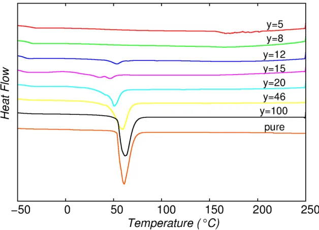
4.1.1 DSC ... 65
4.1.2 Relaxation ... 67
4.2 Solid Triblock Copolymer Electrolyte PS-PEO-PS/LiTFSI ... 80
4.2.1 The Polymer PS-PEO-PS ... 80
4.2.2 The Salt LiTFSI ... 85
4.3.1 7Li NMR Spectroscopy of PEGD-LiClO4 (y = 5) ... 93
4.3.2 Multiple Quantum Coherence Excitation ... 94
4.3.3 Multiple Quantum Coherence Detection... 96
4.3.4 Multiple Quantum Pulse Gradient Measurements ... 99
5 Conclusions and Outlook ... 103
1
Introduction
One of the biggest challenges in modern materials science and engineering is to develop new materials, which satisfy the increasing demand on production, storage and transport of energy. High volumetric and gravimetric energy density and lightweight make lithium ion batteries interesting for these applications. (1-2) Lithium metal batteries (where lithium metal is the anode material) are of great interest, since they present the highest energy density among the different types of batteries. (3) Nevertheless, due to dendrite formation, this type of battery is related with serious safety issues: dendrite formation can lead to short-cuts and destruction of the battery. (3) An approach to overcome this safety issue is the use of solid polymer electrolytes, since electrolytes with large mechanical stability can avoid dendrite formation. (4)
Since the discovery of ionic conductivity in PEO/Na+ (PEO, poly(ethylene oxide)) in 1975 by Wright (5) and the subsequent suggestion by Armand (6) of using ion conducting polymers as solid electrolytes in lithium ion batteries, this research field has attracted a lot of interest in the scientific community. (7–11) Conducting polymers via lithium ions present various advantages as electrolytes in batteries such as safety and higher design flexibility. Nevertheless, it is still a challenge to improve their electrochemical properties. (12)
The mechanical stability of PEO is not sufficient to completely avoid dendrite formation. In this context, synthesis of block copolymers becomes interesting, since it allows combining components with different properties. For instance, in the triblock copolymer PS-PEO-PS, ionic conductivity is guaranteed by the PEO block, in which salts can be dissolved, while the polystyrene (PS) blocks account for mechanical stability. (4,13–18) Commonly, an improvement in ionic conductivity, obtained by an increment of the PEO percentage in the copolymer comes along with a decrease of mechanical stability. (13) Consequently, it is necessary to find a compromise between good ionic conduction and sufficient mechanical resistance avoiding dendrite formation.
in. (19-20) This makes NMR a useful experimental tool, which allows studying the charge carrier as well as the host matrix of ion conducting materials independently. From those studies, it is possible to obtain information such as kind and number of diffusing ions, activation energies, jump rates or correlation effects, as well as structural and morphological properties. (20-21)
Transverse relaxation is mediated by fluctuations of the local magnetic fields in proximity of the nuclei. These fluctuations originate from the rotational and translational motions of the nuclei. In this way, nuclei with different motional freedom can have different transverse relaxation times (T2). The CPMG technique (named after they developers Carr-Purcell-Meiboom-Gill) (22-23) allows measuring T2 relaxation time distributions. Measurements of T2 relaxation times can contribute to understand the dynamic processes involved in ionic conductivity. (20)
The two-dimensional exchange experiment T2xT2, obtained by concatenating two CPMGs and its one-dimensional variants, (24–27) allow to correlate sites with different transverse relaxations. This makes it possible to obtain information on the possible diffusive paths, and even to characterize their specific exchange rates. (26) Relaxation exchange, in contrast to conventional Fourier transform exchange experiments, does not require different precession frequencies of the involved sites but different relaxation rates. In many cases, heterogeneities of the sample do not reflect on chemical shift differences. Relaxation exchange experiments have mainly gain popularity in the field of porous media such as reservoir rocks, (24,28-29) cements, (30) bones (31) or ceramics, (27) but have also been used in a large variety of areas, like biological tissue (32-33) or proton exchange membranes. (34) To our knowledge, they have not been used to characterize the ions in polymer electrolytes. The here presented ion conducting polymers present a 7Li spectrum with signals with strongly overlapping chemical shifts, while the T2 relaxation time distribution clearly differentiates two sites.
triblock copolymer Poly(ethylene glycol-400) distearate (PEGD) doped with large amounts of LiClO4, which presents order in the polymer matrix even at temperatures above the melting temperature.
Goal of this Thesis
The Li-doped ion conductor poly(ethylene glycol) PEG has, between the glass transition temperature (Tg) and the melting point (Tm), at least two phases, vitreous and crystalline. Being the first the principal responsible for the ionic conductivity. In the first part of this work, we apply NMR relaxometry techniques aiming to develop a methodology for studying the Li+ ions in the amorphous phase. In particular, we propose the use of 7Li T2 relaxation time measurements to study dynamical behavior of the lithium ions and the use of T2xT2 exchange experiments, to quantify exchange rates between the two different found Li+ sites.
In a second part, after validating the relaxometry techniques, we aim to apply them to a more advanced material, of higher complexity, Li-doped triblock copolymers based on poly(ethylene oxide). The triblock copolymer PS-PEO-PS has promising properties for applications as solid polymer electrolyte in lithium metal batteries. It has a lamellar structure, where aliphatic and polar chains form separated layers. Before applying the previously studied relaxometry techniques, it was necessary to gain knowledge about morphological and structural properties of these samples. Therefore, they were studied with high-resolution solid-state NMR techniques. Spin diffusion experiments allowed determining domain sizes of the heterogeneous segments of the block copolymer. Rotating frame relaxation (T1ρ) allowed studying dynamical processes of the spectroscopic distinguishable phases. With the combination of the results from 1H and 13C spectroscopy and 7Li relaxation measurements, we hope to gain new insights on the mechanisms involved in the ion conduction in the polymer matrix.
NMR spectroscopy techniques applied on polymers in the group of Prof. Klaus Schmidt-Rohr.
2
Theoretical Background
2.1
Ion Conducting Polymers
2.1.1 Basic Concepts of Polymers
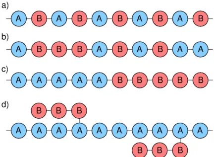
Polymers are macromolecules of large molecular weight composed of repeat units. They could be either organic, inorganic or even hybrids, but in this work we will focus only on organic polymers. The molecular weight of a polymer will depend on the molecular weight of the repeat unit and the number of times it repeats. Due to the polymerization process polymers could have strong heterogeneity in the degree of polymerization, or polydispersity. Therefore, the polymer molecular weight will be given as an average value of the sample. (41) There are multiple ways the repeat units can be aligned along the chains. This alignment will strongly affect their chemical, physical and mechanical properties. They can be aligned as linear polymers without ramifications, forming single chains. If the main chains present some ramifications, they are called branched polymers. In crosslinked polymers the main chains are joined one to another by the ramifications at various points. (41)
Figure 1 - Schematic representations of a) alternating, b) random, c) block and d) graft copolymers composed of two repeat units A and B.
Source: By the author.
Crystallinity in polymers is complex due to the magnitude of the involved molecules. As a consequence of their size and heterogeneity polymers are often semicrystalline, which means they are partially crystalline and partially amorphous. Besides the chemical composition and the molecular structure (linear polymers have a higher tendency to crystallize), the degree of crystallinity of a polymer depends strongly on its thermal history. (41) Furthermore, the presence of chemical distinct phases, in block copolymers or in semicrystalline systems can lead to self-organized systems with microphase-separated structures. The morphology and the domain size of the segregated phases will depend on their ratio and nature. Typical encountered morphologies are spherical, cylindrical, double gyroidal or lamellar. (42-43)
2.1.2 Solid Polymer Electrolytes
Introduction
of carbon instead of lithium metal reduced considerably the high security risks related to the later one. On the downside, the substitution of the anode material reduced the energy density of the electrochemical devices. Therefore, another approach involved replacing the liquid electrolyte by a solid electrolyte, which could mechanically avoid the formation of dendrites and allow the use of lithium metal as anode. In this context ion conducting polymers represent a promising option as electrolytes of high ionic conductivity paired with mechanical robustness and were therefore termed solid polymer electrolytes (SPE) (3).
PEG/PEO doped with Lithium Salts
In 1975 Wright (5) first reported ionic conductivity in a polymer-salt system, PEO/Na+ (PEO, poly(ethylene oxide)). Soon after, Armand (6) suggested the use of ion conducting polymers as solid electrolytes in rechargeable batteries. The presence of oxygen atoms in the PEO (or PEG, poly(ethylene glycol)) structure makes the chains polar, allowing good dissolution of lithium ions in its matrix. The salt concentration in this type of systems is commonly given by the oxygen to lithium ratio y = [O]/[Li].
It has been reported that ionic conductivity mainly occurs in the amorphous phase (above the glass transition temperature Tg) (44) and efforts to avoid crystallization have been done ever since. The mobility of the chains enable translational diffusion of the ions in the solid polymer, turning it a good ion conductor and thus a potential electrolyte. Since the lithium ions are close to the PEO oxygen atoms, it is believed that its dynamics are strongly correlated to segmental reorientations of the polymer. (45) But actually, much is still unknown on the chemical structure and ion transport in PEO. (3)
The chain mobility is strongly correlated to the glass transition temperature of the polymer, after which the amorphous region becomes elastomeric. Therefore polymers with low Tg present good ion conducting properties at room temperature. On the other hand, too low Tg values are related with higher tendency to crystallization. In this context, phase diagrams are a valuable tool. A phase diagram of PEO-LiClO4is shown in Gray’s book Solid Polymer Electrolytes. (7) For this system various phases were reported: crystalline complexes (PEO)6:LiClO4 and (PEO)3:LiClO4, crystalline pure PEO, as well as amorphous phases. (7,46)
and PEG have shown a maximal ion conductivity for y = 8 to 10. (47-48) The presence of a maximum occurs due to the action of opposed effects. Increment of salt concentration inhibits the crystallization of the pure PEO, if the compound is completely elastomeric, larger conductivity values will be obtained. (47) Furthermore, the number of charge carriers will increase. On the other hand, too large amounts of salt will cause a reduction of available sites and benefit formation of ion pair clusters. (48) Also, the overall polarity of the samples will increase which in turn will stiffen the polymer chains, reducing their mobility. (48)
However, the mechanical stability of PEO/PEG at high temperatures (60-80°C), where the largest capacities are obtained, is not sufficient to completely avoid dendrite formation. (3)
Triblock Copolymer PS-PEO-PS
Electrolytes with high mechanical stability can stop dendrite growth in Li metal batteries. On the other hand, highest ionic conductivity is present in soft polymers, such as PEO. Several studies have been done, aiming to combine polymers with high shear modulus with polymers with good ion conducting properties, through the synthesis of block copolymers. The group of Balsara (4,13) presented a strategy to obtain copolymers in which mechanical and electrical properties are decoupled. The most common architectures are AB diblock and ABA triblock copolymers, where A is the block responsible for mechanical stability and B is the block responsible for ion conductivity. (11) In polystyrene-poly(ethylene oxide) (PS-PEO) diblock copolymers the mechanical properties will be governed by the aliphatic PS block, while the PS block should have no influence on the electrical properties of the PEO block. The polymer Polystyrene (PS), despite having a low cost, presents good mechanical properties with a Tg of approximately 100°C, thus above the temperature of operation. Since PS has no polar heteroatom in its structure it cannot dissolve the lithium salts in its structure. Most of this copolymers present a lamellar morphology. (4,13,16)
The normalized conductivity n(T) for block copolymers directly indicates the
conductivity efficiency of the PEO block as compared to a PEO homopolymer at the same temperature and is given by:
( )
( )
( )
n
PEO PEO
T
T
f
T
(1)PEO(T) the conductivity of the homopolymer. Thus, n( ) 1T represents the theoretical limit
at which PEO in the block copolymer presents the same conducting properties as the PEO homopolymer. While the conductivity increases with temperature, the normalized conductivity is not affected, indicating that both homopolymer and block copolymer have the same temperature dependency. (13)
Since the ion transport in PEO was related to segmental motions of the polymer chains, the conductivity is expected to be independent of MPEO over a high molecular weight limit. While for the homopolymer this limit is already reached at about 3 kg/mol, (49) for the block copolymer conductivity continues increasing up to at least 60 kg/mol (4) (for LiTFSI and y = 12). Furthermore, for lower doping ratios, the normalized conductivities are considerably lower than the theoretical limit, n( ) 1T , for molecular weights up to 100 kg/mol. (13) As possible explanations for this drastic difference, two different approaches were proposed: First, at the PS-PEO interface the dielectric constant of PEO is lower, which could reduce the degree of dissociation of the salts in this region. (14) And second, block copolymers stretch when they form ordered phases, thus the Li+ ions are tighter coordinated to PEO chains in low molecular weight copolymers than in stretched PEO of high molecular weight copolymers, leaving to increasing conductivity with molecular weight. (16)
Structural and morphological studies of the triblock copolymer PS-PEO-PS without salt showed that the relative amount of the different blocks, at a constant PEO molecular weight of 10 kg/mol, is of crucial importance. (16) The amount of PS will affect the PEO block, in the sense that large amounts will inhibit crystallization of PEO. This could be related to the previous mentioned stretching of the PEO, which limits the capacity of folding of the chains. On the other side, if PEO is the dominant block, the PS block will present larger mobility, which will even become close to that of PEO itself. (16)
Triblock Copolymer Poly(Ethilene Glycol) Distearate (PEGD)
work has low molecular weight (MPEGD = 946 g/mol with MPEG = 400 g/mol), being the chemical formula:
CH3(CH2)16CO(OCH2CH2)9O2C(CH2)16CH3
A B A
Through dissolution of LiClO4, an ion conducing polymer is obtained. Ionic conductivity and thermal properties strongly depend on the amount of salt. (51) An increment in the salt concentration will increase the glass transition temperature Tg of the mobile phase (from Tg = -68°C for pure PEGD to Tg = -20°C for y = 5). On the other hand, the melting point Tm of the stearate phase remains constant (Tm≈ 35°C). (52) The ion conductivity in the melt phase presents a maximum at a doping amount of y = 9. (51)
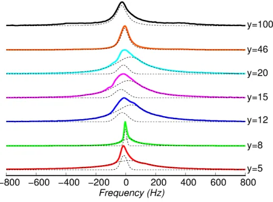
PEGD exhibits an interesting phenomenon, frequently found in block copolymers and polymer liquid crystals, the NMR spectra of highly doped PEGD show a sharp 7Li quadrupolar pattern at temperatures above the polymer melting point. This is attributed to the presence of order in the polymer matrix, which in turn is responsible for anisotropic dynamics of the ions. However, orientation is only observed in the presence of a magnetic field of a few Tesla and with addition of appropriate amounts of salt. (53) This orientation is maintained up to an order-disorder transition temperature TOD, which depends on the doping ratio. For the strongly doped sample with y = 5, TOD≈ 80°C, while for the sample with less LiClO4, y = 9, TOD≈ 46°C. (53) At temperatures around the melting point two phases coexist, thus the obtained 7Li spectra showed two overlapping quadrupole powder pattern. (52) Through annealing of the sample above TOD in the presence of an external magnetic field and subsequent cooling, it is possible to ensure that the sample is completely in the ordered state (53).
2.2
Nuclear Magnetic Resonance
2.2.1 Basic Principles of NMR Spectroscopy
The Nuclear Spin
Nuclei can possess a spin
I
ˆ
. From spin results, as an intrinsic property, an angular momentumJ
ˆ
and a magnetic moment
ˆ
. (19) The spin, angular momentum and magnetic moment operators are related according toˆ
ˆ
ˆ
J
I
(2)being γ the gyromagnetic ratio, a nucleus specific constant. For a single spin, a consistent set of spin operators, Î2, Îx, Îy and Îz, determine all properties. They are related according to:
2 2 2 2
ˆ ˆx ˆy ˆz
I I I I (3)
where Î2 commutes with Îz. Their eigenfunctions,
l m
,
, and eigenvalues, l and m,respectively, are:
2
ˆ , ( 1) ,
I l m l l l m (4)
ˆz , ,
I l m m l m (5)
where the quantum number m may be any of the 2l+1 values l, l - 1, …, -l, and l is either an integer or a half-integer. The eigenfunctions
l m
,
are spherical harmonics. (54) Note that the factor ħ is included as part of the operator as is convenient and common in the NMR literature. (42)In presence of an external magnetic field
B
0
(0,0, )
B
0 , the Zeeman interaction usually dominates the behavior of the nuclear spin system. The Zeeman Hamiltonian is given by:0
ˆ
zH
B Î
. (6)The eigenvalues of the Hamiltonian obtained from the eigenfunctions
l m
,
are the Energies El,m of the different possible states of the spin. Thus, according to:,
ˆ , l m ,
H l m E l m , (7)
the allowed energies are:
, 0
l m
E
B m
. (8)Furthermore, the selection rule of NMR states (55): 1
m
Therefore, the energy difference ΔEbetween two states is given by γψ0. This transition energy
corresponds to the Larmor frequency ( 0 or L).The population difference between the
energy levels corresponds to a magnetization on the z-axis and at equilibrium it is described by the Boltzmann distribution. This difference in energy and population is the basis of NMR. The population, pm, of each eigenstate,
m
, is: (19)' / / ' m m E kT
m E kT
m
e
p
e
. (10)The Density Matrix
It is convenient to describe an ensemble of spin systems through the density matrix ˆ. Each spin system is in one of the possible eigenstates, , with a probability pΨ. Analogously, each spin system in the whole ensemble may be considered to be in the same superposition state, Ψ:
p
. (11)Furthermore, the states of any spin system can be written as a sum over a basis set of functions
m
(for instance the eigenfunctions of the spin operators represent an appropriate basis set):m m
c m
. (12)The expectation value of an operator
Q
ˆ
is:* ' , '
ˆ
ˆ
'
m m
m m
Q
p
c c
m Q m
. (13)Alternatively, it can be written as:
ˆ
Q
Tr
p
Q
, (14)where Q is the matrix representation of
, '
ˆ '
m m
m Q m
. The spin density operator ˆ is definedˆ
p
. (15)Leaving to following expression for the expectation value:
ˆ
ˆ
Q
Tr
Q
. (16)The matrix representation of the density matrix presents some interesting properties. The diagonal elements
ˆ
mm (equation (17)) are the populations of the statesm
while the off-diagonal elements
ˆ
mm' (equation(18)) are the coherences between statesm
and'
m
. (54)* *
ˆ
mmp c c
m mc c
m m
(17)* *
' ' '
ˆ
mmp c c
m mc c
m m
. (18)The overbar indicates the average over all spin systems. At thermal equilibrium the coherences between the states are zero, while the populations satisfy the Boltzmann distribution as given above. (54) The equilibrium spin density matrix is:
0 0 ˆ ˆ
ˆ
(
)
z z B I kT eq B I kTe
Tr e
. (19)Under consideration of the high temperature approximation, which is valid for temperatures above 1 K, (42) the density matrix can be simplified to:
0
1
ˆ
ˆ
ˆ
(1
)
2
eq zB
I
kT
. (20)It is useful to classify the coherences of the density matrix by their coherence order. In the Zeeman basis the order qmm’ of the coherence ρmm’ is defined as: (54)
'
'
mm
q
m m
. (21)Where m and m’ are the eigenvalues of
I
ˆ
z of their respective eigenfunctions, according to equation (5). The maximal coherence order qmax in a spinsystem of n spins I is definedTime Evolution of the Density Matrix
While the spin density operator describes the state of the ensemble of spin systems, any interaction that changes this state is described by a Hamiltonian. The effects caused on the spin density operator are given by the von Neumann (or Liouville-von Neumann) equation: (42)
ˆ
ˆ
,
ˆ
d
i H
dt
. (22)The formal solution of the von Neumann equation for a time-independent Hamiltonian is given by:
ˆ ˆ
ˆ
( )
t
e
iHtˆ
(0)
e
iHt
. (23)
To analyze the effects of the propagators eiHtˆ on the density matrix it is possible to use the Baker-Campbell-Hausdorff Equation:
2 3
ˆ
ˆ ˆ
ˆ ˆ ˆ
ˆ
( )
ˆ
(0)
[ (0), ]
ˆ
[[ (0), ], ]
ˆ
[[ (0), ], ], ] ...
ˆ
2!
3!
t
it
t
it
H
H H
H H H
. (24)Evolution of the Density Matrix under the Zeeman Interaction
It is useful to analyze the free evolution of the density matrix in terms of its populations and coherences considering only the effect of the Zeeman Hamiltonian (
H
ˆ
B Î
0 z
L zÎ
). Therefore, first the density matrix is decomposed in terms of the coherence order q: (56)ˆ
( )
ˆ
q( )
q
t
t
. (25)Subsequently, application of the Hamiltonian on the components leads to:
' ˆ ' ˆ
ˆ
qmm( )
t
e
iHtˆ
qmm(0)
e
iHt
(26)
ˆ ˆ
*
' i tIL z
'
i tIL zm m
c c e
m m e
' *
' L L
'
i tm i tm m m
c c e
e
m m
( ') *
' L
'
i t m m m m
c c e
m m
' '
L mm mm
i tq q
e
This result implies that the Zeeman Hamiltonian will not change the coherence order of any component of the density matrix. Furthermore, the populations are not affected, while the coherences will oscillate with cos(q t i
L ) sin( q t
L ). This represents the precession of the magnetization around the external field B0 and in the case of single quantum coherence it isrelated to the complex observable NMR signal.
The Density Matrix in the Rotating Frame
It will prove useful to eliminate the effect of the Larmor rotation by transition to a frame that rotates with the same frequency: R= L. The rotating frame spin density operator
is related to the fixed frame density operator by: (42)
ˆ
( )
i R ztIˆ
( )
i R ztIR
t
e
t e
. (27)
The Effect of Radio-Frequency Pulses
Transition between the energy levels are induced under the action of an additional magnetic field B1( )t . (42) This time dependent field has to oscillate at a frequency close to the resonance frequency, usually in the radio-frequency (rf) range. The Hamiltonian describing the effect of both the static B0 and the oscillating B1 (which will be taken to
oscillate along the x-axis) fields is:
0 1 0 1
ˆ ˆ ˆ (ˆz 2ˆx cos( rf ))
H H H
I B I B
t . (28)The oscillating B1 field may be described as two counter rotating components. One
component rotates in the same sense as the nuclear spins, while the other rotates in the opposite sense. However, in most cases this second component has no significant effect on the spin system, (19) so that equation (28) can be rewritten as:
0 1
ˆ
(
ˆ
i rftIzˆ
i rftIz)
z x
H
I B
B e
I e
. (29)Furthermore, the Hamiltonian can be transformed into the rotating frame. In a frame rotating about B0 at a frequency rf the Hamiltonian becomes:
0 1
ˆR ( rf)ˆz ˆx
H
I
B I , (30),1 1
ˆR ˆR ˆx
H H
B I . (31)The flip angle caused by the pulse on the spin system is given by:
1 1
rf
B
rf rf
. (32)Application of pulses on a spin system allows changing the coherence order of any component of the spin density matrix, as shown in equation (33) for a pulse of arbitrary phase
φ. For instance, it is possible to excite coherence from a state of thermal equilibrium by applying a pulse.
1( ) 1( ) '
1 2
'
ˆ
( )
ˆ
( )
H t q H t q i q
q
e
t e
t e
. (33)Each coherence component that is transferred by the pulse will gain a phase shift Δqφ, where
Δq is the coherence order difference Δq = q’-q. (56)
Ensemble of Spin 1/2: Pauli Matrices
Consider a sample of magnetically equivalent and independent spins 1/2, which will behave as an ensemble of isolated spins 1/2. An appropriate set of spin operators for such spin systems are the Pauli matrices: (42)
1 0 1 ˆ 0 1 2 z
ˆ 1 0 11 0 2 x
ˆ 1 00 2 y i i
. (34)Furthermore, consider the sample was placed into an external magnetic field, B0, for
enough time in order to reach thermal equilibrium. The spin density matrix in the rotating frame was given in equation (20). Since the unity operator 1ˆ commutes with all operators and
has no importance in most cases it will not be considered in the further discussion. (42) Therefore, the initial state can be written as:
0
1
ˆ
ˆ
ˆ
(0)
2
z zB
kT
. (35)Ensemble of Spin-1/2: A 90° Pulse and the NMR Signal
The effect caused by an rf pulse along the x-axis on the spin system can be described as follows:
1 1
ˆ ˆ
ˆ
(1)
e
irfˆ
(0)
e
irf1 1 1 1
1 1 1 1
cos( ) sin( ) 1 0 cos( ) sin( )
1 2 2 1 1 2 2
ˆ(1)
0 1
2
2 2
sin( ) cos( ) sin( ) cos( )
2 2 2 2
rf rf rf rf
rf rf rf rf
i i i i .
Thus, for a flip angle rf = 90°:
1 1 0 1
1 1 1
ˆ(1)
1 2 0 1 1
2 2 i i i i
(37) 0 1 ˆ ˆ(1) 0 2 y i i
.The pulse equalized the populations of the two states and furthermore, converted the population difference into coherences. (54) Finally, after the pulse the magnetization is allowed to evolve freely under the Zeeman interaction:
1 1
ˆ ˆ
ˆ
(2)
e
iH tzˆ
(1)
e
iH tz
(38)
1
1 1 1
0
1
ˆ
ˆ
ˆ
(2)
cos(
)
sin(
)
2
0
L
L
i t
y L x L
i t
i e
t
t
i e
.Note that the solution of equation (26) was used and the coherence order here is qmm’ = 1. This final expression is proportional to the quadrature-detected NMR signal, which is obtained by taking the trace Tr(
ˆˆ), withI
ˆ
ˆx i
ˆy. The NMR spectrum can beobtained by Fourier transformation of the quadrature signal. (42)
Ensemble of Spin 1/2: The Spin Echo
The spin echo is obtained by application of a 180° pulse (for instance along the x-axis) while the magnetization is in the transverse plane:
1 180 1 180
ˆ ˆ
ˆ
(3)
e
iˆ
(2)
e
i
(39)
1 1
ˆ
ˆ
ˆ
(3)
ycos(
Lt
)
xsin(
Lt
)
.After the pulse the magnetization evolves freely again:
2 2
ˆ ˆ
ˆ
(4)
e
iztˆ
(3)
e
izt
, (40)ˆ
ˆ
(4)
yˆ
(1)
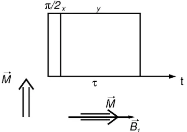
. (41)The spin echo is useful for refocusing the Zeeman interaction, heteronuclear dipolar coupling and magnetic field inhomogeneities. (42) The total pulse sequence is shown graphically in Figure 2.
Figure 2 - Spin Echo pulse sequence. Source: Adapted from SCHMIDT-ROHR.(42)
Nuclear Spin Interactions
Until now, the spin system was described just in terms of the Zeeman interaction; however, the Zeeman interaction contains no relevant structural information itself. Each nucleus feels magnetic and electric fields originating from the sample, which are crucial for spectroscopic applications. (57) These interactions are included in the internal spin Hamiltonian
H
ˆ
int given as:int
ˆ ˆCS ˆDD ˆJ ˆQ
H H H H H (42)
of the quadrupolar coupling and represents the electric interaction of a nuclear electric quadrupole moment with the surrounding electric field gradient. (54)
The internal nuclear Spin interactions can be written in a general form as:
ˆ
ˆ
ˆ
int locH
IA J
(43)where Iˆ is a nuclear spin vector,
J
ˆ
is the source of the local magnetic field at the nucleus which may be originated by either another spin, of equal or different nature, or the external magnetic field and Aloc is a second-rank Cartesian tensor which describes the strength andorientation dependence of the local spin interaction. (19)
Irreducible Spherical Tensor Operators
Before further describing the nuclear spin interactions it will be useful to introduce the concept of spherical tensor operators. In some cases, due to some specific symmetry properties of the spherical tensor operators, this formalism has some advantages over the classical Cartesian spin operators I Iˆ ˆx, y and
I
ˆ
z. For a rank l there are 2l + 1 different spherical tensor operatorsT
ˆ
lm with order m l l, 1,...,l1,l. A specific and useful symmetry property of the irreducible spherical tensor operators is that under rotations their rank does not change and the result of the rotation can be expressed as a linear combination of irreducible tensor operators of the same rank as the initial. (19)In this work the irreducible tensor operator formalism was used to calculate excitation of multiple quantum coherences for 7Li, a spin 3/2 nucleus. Therefore, the necessary commutation relations of the Baker-Campbell-Hausdorff equation (shown previously, equation (24)) were based on the articles published by Bowden and Hutchison. (58-59)
The internal nuclear spin interaction in terms of the irreducible spherical tensor operators is given as:
2
, 0
ˆ ˆ
ˆ l 1 m ˆ
int loc l m lm
l m l
H T
IA J =
(44)Chemical Shift
The presence of an external magnetic field induces electronic currents in a molecule. Those will in turn generate a local magnetic field
B
s. (42) The interaction of the local fieldwith the nuclear spin is called the shielding interaction and it can alter the nuclear resonance frequency. This shift of the resonance frequency is called chemical shift. (19) The induced local field is linearly dependent on the applied field: (54)
s 0
B
B
(45)where is the chemical shift tensor, a 3x3 matrix. The chemical shift Hamiltonian acting on a spin is:
ˆ
ˆ
CSH
I B
0. (46)Direct Dipole-Dipole Coupling
The magnetic moments of the nuclei interact through space, this interaction is called direct dipolar coupling (in contrast to the indirect dipolar coupling which is mediated by electron clouds). The Hamiltonian of the direct dipolar interaction between two nuclear spins, i and j, is given by
0
3
ˆ
ˆ
ˆ ˆ
3(
/ )(
/ )
ˆ
4
( )
i j i j
ij ij ij ij
DD i j
ij
r
r
H
r
I
r
I
r
I
I
(47)where 0 is the permeability of vacuum,
r
ij the vector between the two nuclei andij ij
r r . (42) Alternatively, it is possible to resume the dipolar interaction into a second rank
Cartesian tensor D to rewrite the equation as:
ˆ ˆ
ˆ
i jDD
H
I DI
(48)or, in terms of a spherical tensor operator (19):
20 20
ˆ
DDˆ
H
T
. (49)In an isotropic liquid, the secular components (components of the Hamiltonian which commute with
Î
z) of the dipole-dipole coupling are essentially averaged out to zero. In solids,Quadrupolar Coupling
Nuclei with a spin larger than 1/2 have in addition to the magnetic dipole moment an electric quadrupole moment, which interacts with the electric field gradient generated by the electron clouds surrounding the nuclei. This will have an effect on the nuclear spin system. The quadrupole interaction Hamiltonian is given by:
ˆ ˆ
ˆ
2 (2
1)
Q
eQ
H
I I
IVI
(50)where V is the electric field gradient tensor, e the elementary charge and Q the quadrupole
moment. (42) Thus, eQ is constant for a given nuclear isotope. The magnitude of the quadrupolar interaction will depend strongly on the molecular environment, for instances, symmetrical ionic environments will present small local field gradients and consequently the nuclei in such an environment will have small quadrupolar couplings. (54)
The quadrupolar couplings appearing in this work, from the quadrupolar moment of the spin 3/2 nucleus 7Li, are small and therefore can be treated as perturbations of the Zeeman interaction. Furthermore, only the secular term HˆQ(1) will be considered, leaving to: (54)
(1) (1) 1 2 ˆ
ˆ (3ˆ ( 1)1)
6
Q Q z
H
I I I (51)with
Q(1), the first-order quadrupolar coupling given by:(1)
3
2 (2
1)
ZZ Q
eQV
I I
. (52)If the Cartesian spin operators are replaced by spherical tensor operators, the first order quadrupolar coupling Hamiltonian can be written as: (19)
(1)
20 20
ˆQ ˆ
H V T . (53)
Quadrupolar nuclei have more than two angular momentum eigenstates along the z-axis, according to equation (5) for spin 3/2 there are four eigenstates. Figure 3 shows the energy levels of a spin 3/2 nucleus and the effect of the quadrupolar coupling to first order. The relative intensities of the peaks of the central and satellite transitions at – Q/2, 0 and Q/2
Figure 3 - Effect of the quadrupole coupling to first order on the Zeeman interaction for a spin 3/2. ω0 is the
Larmor frequency and ωQ the quadrupole coupling.
Source: By the author.
The relevant Cartesian
I I
ˆ ˆ
x,
y andI
ˆ
z and irreducible spherical spin operators for spins3/2 are given in their matrix representation Figure 4 and Figure 5: (60)
3 0 0 0 0 1 0 0 1
ˆ
0 0 1 0 2
0 0 0 3
z
0 3 0 0 3 0 2 0 1
ˆ
2 0 2 0 3 0 0 3 0
x
0 3 0 0 3 0 2 0 1
ˆ
2 0 2 0 3 0 0 3 0
y i
1,0
3 0 0 0 0 1 0 0 1
ˆ
0 0 1 0 2 5
0 0 0 3
2,0
1 0 0 0 0 1 0 0 1
ˆ
0 0 1 0 2
0 0 0 1
3,0
1 0 0 0 0 3 0 0 1
ˆ
0 0 3 0 2 5
0 0 0 1
1,1
0 1 0 0 2
0 0 0
3
ˆ 3
10
0 0 0 1 0 0 0 0
2,1
0 1 0 0 0 0 0 0 1
ˆ
0 0 0 1 2
0 0 0 0 3,1
0 1 0 0 1 0 0 3 0 ˆ
5 0 0 0 1 0 0 0 0
2,2
0 0 1 0 0 0 0 1 1
ˆ
0 0 0 0 2
0 0 0 0
3,2
0 0 1 0 0 0 0 1 1
ˆ
0 0 0 0 2
0 0 0 0
3,3
0 0 0 1 0 0 0 0 ˆ
0 0 0 0 0 0 0 0 .
Figure 5 -Irreducible tensor operators ˆlm of rank l and order m for a single spin 3/2. Source: By TELLES. (60)
2.2.2 NMR Spectroscopy Experiments
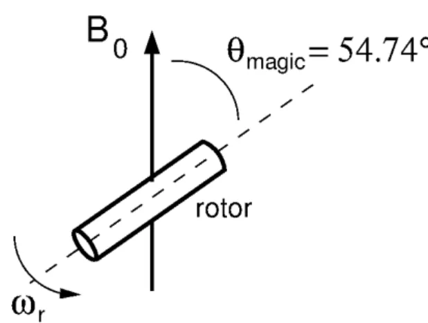
Magic Angle Spinning (MAS)
Magic Angle Spinning (MAS) is a technique used in most solid state NMR experiments. In MAS experiments (Figure 6) the sample is placed in a rotor and rotated about an axis oriented at the magic angle with respect to the external magnetic field ( magic = 54.75°). The aim of this technique is to average out the effect of the anisotropic
Figure 6 - Spinning of a sample around an axis oriented at the magic angle
magicwith respect to the externalmagnetic field.
Source: By the author.
The general condition which has to be satisfied, in order to have an efficient removal of the anisotropic effects, is that the spinning frequency of the rotor is fast compared to the spectral linewidth. However, if the spinning frequency is not sufficiently large, the spectrum will present extra lines. These lines are separated by a frequency equal to the spinning frequency or integer multiples of it, called spinning sidebands.
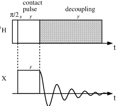
Cross-Polarization
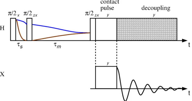
Figure 7 - Pulse sequence of the cross-polarization experiment X{1H} with heteronuclear decoupling.
Source: By the author.
First, a π/2 pulse flips the 1H magnetization into the transverse plane. Parallel to the magnetization an on-resonance 1H contact pulse is applied, the resulting field B1(1H) is called spin-lock field. This field has two functions, it locks the magnetization and it acts as quantization axis for the 1H spins. However, the weaker B1(1H) field is not able to lock the same amount of polarization as the external magnetic field.
At the same time, an analogue B1(X) spin-lock field is applied, which acts as quantization axis for the X spins. At the beginning, the two X states are equally populated. The dipolar coupling, which only contains operators acting on the z-axis, cannot affect the net energy of the spin system in the rotating frame. Thus, a transition from the energetic lower state into the energetic higher state of a 1H spin in the rotating state is compensated by the dipolar coupling through the opposite transition of an X spin, but can only occur if the energy gap in both transitions is equal. Therefore the Hartmann-Hahn condition (equation (54)) has to be fulfilled, which experimentally implies that the spin-lock fields have to be set carefully. (19)
1
1
(
)
1( )
H
B H
xB X
. (54)heteronuclear dipolar couplings of the 1H spins on the X spins. This technique is called heteronuclear decoupling.
T1ρ Measurement
For measuring the longitudinal relaxation time in the rotating field, T1ρ, the magnetization is locked by the
B
1 field during a time in the spin-lock experiment (Figure 8).(42) The magnetization along the locking field will not experience dipolar dephasing and therefore decay only due to the relaxation in the rotating time with the time constant T1ρ. Since
B
1 is much smaller thanB
0, T1ρ will be sensible to different molecular motions than T1, in the order of tens of kHz instead of hundreds of MHz (42).Figure 8 - Pulse sequence of the spin-lock experiment for measuring T1ρ.
Source: Adapted from SCHMIDT-ROHR.(42)
Spin Diffusion
Spin diffusion is the diffusion of coherent magnetization without the diffusion of matter and is mediated by dipolar couplings. (19) The time dependence of the diffusion process contains information on the domain sizes and morphology in heterogeneous polymers. (42) The spin diffusion experiment allows to determine distances in a range from 0.1 to 200 nm. In Figure 9, the pulse sequence of the 1H Goldman Shen experiment is shown (with subsequent CP and 13C{1H} detection and heteronuclear decoupling).
transverse relaxation can be used, which itself is due to dipolar couplings. (42,61) Therefore, first a π/2 pulse flips the magnetization in to the transverse plane, then the system is allowed to evolve freely until only magnetization from the mobile region remains. A second pulse stores the magnetization in the z-axis and during a time tm, the 1H spin diffusion occurs.
Finally, the last pulse brings the magnetization back to the transverse plane for detection. The tm dependence of the magnetization increment gives direct information of the domain
sizes. (42)
Figure 9 - Pulse sequence of the Goldman-Shen spin diffusion experiment with CP and heteronuclear decoupling.
Source: By the author.
To analyze the diffusion curves, a diffusion model considering Fick’s second law is used. For a two component system it is useful to apply the initial rate approximation since it simplifies the problem by assuming an initial linear dependence of the signal intensity with
m
t . The average size of the mobile phase dMP can be obtained as
,0
4
s
RP MP m
MP
RP MP
D D t
d
D D
(55)
part of the curve with the equilibrium value. Subsequently by dividing by the volumetric fraction
RP we obtain,0 s m s m RP t t
. (56)
DRP and DMP are the spin diffusion coefficients of the rigid and mobile phase
respectively. In this work, for the rigid phase (PS) DRP = 0.8 nm2/ms was used, as indicated in
literature, (62) while for the mobile phase (PEO) it was calculated according to 6 1,5
2
8.2 10
0.007
MP
D
T
(57)Finally, the inter-domain distance is determined by following relationship: (42)
MP MP I MP MP d d d
(58)
2.3
Relaxation in NMR
2.3.1 Theory of Relaxation
Autocorrelation Function and Spectral Density
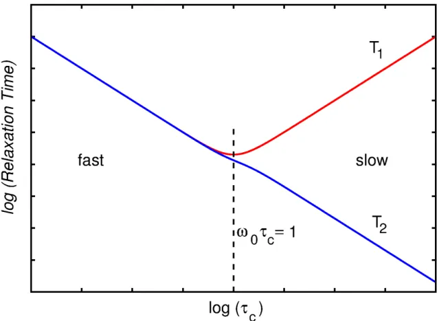
Nuclear Spin Relaxation is an incoherent effect, and thus not reversible. Relaxation is caused by the distribution of local fields and depends on their magnitude as well as on their fluctuation rates. (42,63) This dependency was first described by Bloembergen, Purcell and Pound in the so called BPP theory. (64)
Fluctuations of the local magnetic fields may be caused, for example, by molecular reorientations. The ergodic hypothesis states that the average over an ensemble of particles is equal to the average of a single particle over time. Figure 10(a) shows a rapid and a slow randomly fluctuating function f(t). The average in this model will supposed to be zero. In general, the fluctuation behavior of a randomly fluctuating function f(t) can be described in terms of its autocorrelation function G( ). Suppose a function as follows: (54)
( )
( )
(
)
G
f t f t
. (59)/
( )
(0)
cG
G
e
. (60)The spectral density J( ) is defined as the Fourier transform of the autocorrelation function (54)
2 2
( ) 1
c
c
J
. (61)
In the case of fast fluctuating fields, the spectral density is broad, while for slow fluctuating fields it is sharp (Figure 10(c)). Nonetheless, the area under the curve does not depend on c.
Figure 10 - Fast and slow random fluctuations between two sites (a) and their respective autocorrelation function (b) and spectral density (c).
Source: Adapted from LEVITT. (54)
Transition Probabilities
Consider a system of spin 1/2 nuclei, which in the presence of an external magnetic field will have two possible energy eigenstates
m
,1/ 2
and
1/ 2
, with populations p+and p- respectively and N pp. A perturbation, such as the presence of an alternating
from state
1/ 2
to
1/ 2
is denoted W- and the reverse transition W+ (Figure 11). Thus theevolution of the population p+ is given by following equation: (65) dp
p W p W
dt
. (62)
Figure 11 - Transition probabilities between two energy eigenstates of a spin 1/2 in the presence of an external magnetic field.
Source: By the author.
Time-dependent perturbation theory predicts that the transition probabilities induced by an interaction V(t) between two states of different energies in one direction and in the reverse direction to be equal, (65) thus W WW, which simplifies equation (62) to:
( )
dp
W p p
dt
. (63)
Let us define a variable, n, describing the population difference between both states n p p. The kinetic equation for the population difference is obtained straightforwardly:
2
dn
Wn
dt , (64)
whose solution is:
2