ABSTRACT: The application of quantitative methods to digital soil and geomorphological map-ping is becoming an increasing trend. One of these methods, Geomorphons, was developed to identify the ten most common landforms based on digital elevation models. This study aimed to make a quantitative assessment of the relationships between Geomorphons units, determined at three spatial resolutions and nine radii, and soil types and properties of two watersheds with different soil-landscape relationships in Brazil to help soil surveying and mapping under tropical conditions. The study was conducted at Lavrinha Creek (LCW) and Marcela Creek (MCW) wa-tersheds, located in the state of Minas Gerais, Brazil. Spatial resolutions of 10, 20 and 30 m were the basis for generating Geomorphons at 9 radii of calculation for the watersheds. They were overlapped to detailed soil maps of the watersheds and a chi-square test was carried out to assess their relationship with soil types. Observation points were compared with the most highly correlated Geomorphons to also assess relationships with soil properties. Geomorphons with resolution of 30-m and radii of 20 and 50 cells, respectively for LCW and MCW, were more highly correlated with the variability of soil types, in accordance with the terrain features of these watersheds. The majority of observation points for each soil type was located in the same Geomorphon unit that was dominant when analyzing soil maps. There was less variability in soil properties between Geomorphon units, which was probably due to the highly weathered-leached stage of soils. Geomorphons can help to improve soil maps in tropical conditions when assess-ing soil variability due to its high correlation with tropical soil types variability.
Keywords: Geomorphons, soil-landscape relationships, pedology, landforms, digital soil mapping 1Federal University of Lavras − Dept. of Soil Science, C.P.
3037 − 37200-000 − Lavras, MG − Brazil. 2Federal University of Lavras − Dept. of Engineering. 3Purdue University − Dept. of Agronomy − Lily Hall of Life Sciences, 915 W. State St. − 47907-2054 − West Lafayette, IN − USA.
*Corresponding author <niltcuri@dcs.ufla.br>
Edited by: Silvia del Carmen Imhoff
Geomorphometric tool associated with soil types and properties spatial variability at
Sérgio Henrique Godinho Silva1, Michele Duarte de Menezes1, Carlos Rogério de Mello2, Helen Thaís Pereira de Góes1, Phillip Ray
Owens3, Nilton Curi1*
Received July 22, 2015 Accepted September 17, 2015
Introduction
In soil surveys, the understanding of existing rela-tionships between soil types and/or properties and land-scape features are fundamental to defining the most rep-resentative places for soil morphological description and sampling. This understanding is also needed for digital soil and geomorphological mapping (Bishop et al., 2012). However, due to variations in these relationships from region to region, adjustments to the general geomorphol-ogy models are required for fitting soil variability into an area of interest (Birkeland, 1999).
The advent of digital soil mapping tools has pro-moted a rise in global interest in more detailed soil maps (Vaysse and Lagacherie, 2015) and a transition from quali-tative to more quantiquali-tative soil mapping methods (McBrat-ney et al., 2003). This has been proposed as an approach to exposing the soil scientist's mental (qualitative) model (Bui, 2004) of soil distribution in the landscape through the map-ping process. Applying it to more quantitative methods, this knowledge can be made explicit on maps, resulting in improvements in existing maps, and these relationships can be understood by other soil scientists.
The majority of these recently created mapping tools were developed in countries whose soils are quite different from tropical soils (Schaetzl and Anderson, 2005) for which these tools have to be evaluated and adjusted for improved modeling soil variability. One of these tools
is the Geomorphons, created by Jasiewicz and Stepinski (2013). It consists of a quantitative method for stratifying the landscape in its ten most common landforms. Thus, since relief influences soil properties (Jenny, 1941), its analysis through Geomorphons, after a regional evalua-tion, could lead to improvements in soil survey and map-ping, mainly for countries such as Brazil, where there is a lack of both soil data and financial support for performing detailed soil surveys (Mendonça-Santos and Santos, 2007).
This study was carried out in response to the need for more detailed soil maps in Brazil and other devel-oping countries. It aimed to quantitatively assess the relationships between Geomorphon units, calculated at three spatial resolutions and nine radii, and soil types and properties of two watersheds with different soil-landscape relationships in Brazil to help soil surveying and mapping under tropical conditions.
Materials and Methods
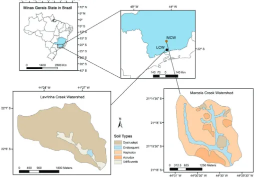
This study was conducted at Lavrinha Creek (LCW) and Marcela Creek (MCW) Watersheds. Table 1 and Figure 1 contain their characterization and location, respectively. The two watersheds are components of the Grande River Basin, important for supplying water to the Grande River, which, in turn, contains a number of hydroelectric power plants and, thereby, generates elec-tric energy for great part of southeastern Brazil (Beskow
et al., 2009). This country has faced a scarcity of water in many states over the last two years, which has drawn attention to watersheds due to their environmental im-portance in water recharge, which is highly influenced by land use and management practices.
LCW is representative of the Mantiqueira Range region, being a headwater watershed, with Dystrudepts (DT) (soils classified according to Soil Taxonomy (Staff, 1999)) developed from gneiss in the sloping area and Udifluvents (UT) and Endoaquents (ET) in the lowest places in the landscape (Menezes et al., 2014). MCW is included in the physiographical region of Vertentes Fields, with gentler slopes compared with LCW. MCW soils were developed from mica schists, where Hapludox (HX) and Acrudox (AX) are found in higher places, DT on steep portions of the landscape, and ET in lower ar-eas of the watershed (Motta et al., 2001). The soil maps
of those watersheds at a detailed scale (LCW: 1:20,000; MCW: 1:12,500) were used as bases for comparing dif-ferent Geomorphons.
For the creation of Geomorphons (Jasiewicz and Stepinski, 2013), Digital Elevation Models (DEMs) with resolutions of 10, 20 and 30 m were created from con-tour lines at a 1:50,000 scale (IBGE) using Topo to Ras-ter tool in ArcMAP 10.1 (ESRI). From these DEMs, the Geomorphons were generated on the following website <http://sil.uc.edu/geom/app> at nine radii (5, 7, 10, 15, 20, 25, 30, 40, and 50 cells), which correspond to the number of cells (pixels) in the radius of the circumfer-ence around a cell of interest used for determining the Geomorphon unit (GU) of that cell of interest. Geomor-phons identifies the ten most common landform units within the landscape, namely, Flat, Peak, Ridge, Shoul-der, Spur, Slope, Footslope, Hollow, Valley and Pit. The
Table 1 − Characterization of the two studied watersheds.
Characteristics Watersheds
Lavrinha Creek Marcela Creek
Location (coordinates) Between longitudes UTM 553800 and 557867 m and latitudes 7554419 and 7551367 m, zone 23K Between longitudes UTM 552591 and 550230 m and latitudes 7648373 and 7651231, zone 23K
Area (ha) 676 ha 470 ha
Altitude (m) From 1151 to 1687 m From 957 to 1057 m
Climate1 Cwb - rainy temperate, semitropical of altitude Cwa - rainy temperate, with dry winters and rainy summers
Mean annual temperature2 15 °C 19.7 °C
Mean annual precipitation2 2,000 mm 1,300 mm
Mean slope gradient (%) 37 12
Parent material Gneiss Mica schists
Native vegetation Atlantic Forest (Rain forest) Cerrado (Brazilian Savanna)
1According to Köppen classification system; 2Mello et al. (2015).
three pixel sizes, the nine radii, and the two watersheds made up a total of 54 Geomorphons maps created for the purpose of analysis.
The soil maps of the two watersheds and the 54 Geomorphons maps were overlapped and the combina-tion of each GU, from the ten most common ones, with the soil polygon on the soil maps had its area calculated. Then, a chi-square test at 5 % probability was conducted (formula presented below) to assess whether there was a relationship between the GUs and the soil types under these different conditions.
X2 o e
2 =
∑
( − )e
in which o is the observed area of each combination be-tween soil types and GUs, and e is the expected area of each combination. The higher the calculated value (X2)
above the critical value (X2 critical) as determined by
a chi-square table, the closer the relationship between soil types and GUs. LCW and MCW, respectively, have three and four soil types that were combined with the 10 possible GUs. Thus, the degree of freedom (DF) for them were, respectively, 29 and 39 (DF = [number of soil types × number of GUs] - 1). Next, analyses of the relationships between the best Geomorphons and the soil types were performed for each watershed in order to clarify the quantitative soil-landscape relationships.
Furthermore, observation points, where mor-phological soil description and classification were per-formed, were inserted on the Geomorphons maps that presented the strongest relationships with the soil types in order to evaluate whether the soils found at these points agreed with the results derived from the analyses of soil maps against GUs, since soil polygon maps allow for a degree of uncertainty of soil classes within each polygon (Soil Survey Manual, 1993). Thirty-seven points were analyzed in LCW and twenty-nine in MCW.
To test whether soil properties also vary according to GUs, an independent data set containing particle size dis-tribution analyses at 0-20 cm depth for the two watersheds, containing 197 points at LCW and 165 at MCW, was insert-ed in sequence in the most highly correlatinsert-ed Geomorphons maps. Next, a Scott-Knott test at 5 % probability was con-ducted using SISVAR 5.3 software to assess the statistical differences in sand, silt, and clay content between the GUs.
Results and Discussion
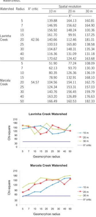
Table 2 and Figure 2 show the chi-square calcu-lated for each pixel size and Geomorphons radius for each watershed.
It was observed that the pixel size alone had great influence on chi-square values and, consequently, the correspondence between soil types and GUs. As an ex-ample, in Table 2, the chi-square in MCW with a radius of five and pixel size of 10 m did not present a relation-ship with the soil types as it was lower than critical X2,
but the pixels measuring 20 and 30 m did (Figure 3). This
Table 2 − Chi-square values calculated for the combinations of pixel sizes and Geomorphons units with soil types of the two studied watersheds.
Watershed Radius X2 critic Spatial resolution
10 m 20 m 30 m
--- X2
---Lavrinha Creek
5
42.56
139.88 164.13 160.81
7 146.95 156.62 164.90
10 156.92 148.24 100.36
15 161.70 99.91 137.25
20 140.66 112.46 181.01
25 100.53 165.80 138.58
30 104.87 148.31 135.34
40 116.36 131.09 131.18
50 170.62 124.42 163.68
Marcela Creek
5
54.57
51.90 77.24 108.09
7 62.13 93.70 130.30
10 80.35 126.36 136.19
15 78.90 132.91 168.10
20 104.56 154.11 162.75
25 124.34 153.31 157.03
30 140.76 156.45 159.79
40 163.20 126.89 176.63
50 166.49 160.53 182.33
Figure 2 − Chi-square for the two watersheds calculated from varying pixel size and Geomorphons radius to assess their correspondence with soil types.
For both watersheds, spatial resolution of 30 m had a better relationship with the soil types than the other pixel sizes. As observed by Roecker and Thomp-son (2010), the more detailed resolutions presented less correspondence to soil types than the coarse resolution, in this case, 30 m. At LCW, where the slope is more variable, it was expected that more detailed resolutions would better represent the landscape (Hengl, 2006), since these conditions should be expressed by more pix-els per unit of area, but the findings of this study show the opposite.
In turn, the Geomorphons radii were also respon-sible for changes in degrees of relationship between soil types and GUs (Table 2). As presented in Figure 4, as the radius increases, the polygons of certain GUs be-come larger. For LCW, for example, at radii of five, 20 and 50 cells at pixel size of 20 m, all of them presented correspondence with soil types for having an X2 greater
than critical X2, although they look different from one
another (Figure 4). In general, at the longest radius, the GUs correspondent to both low and concave places (Footslope, Valley, Pit, and Hollow), ridges (Shoulder, Ridge and Peak) and convex backslopes (Spur) had larger areas than in the other radii. On the other hand, GUs correspondent to flat places (Flat) and linear backslope (Slope) decreased as the radius increased. Furthermore,
it is important to highlight the adequate definition of the watershed limits by Peak and Ridge GUs.
According to the chi-square test at 5 % probability (Table 2), at both LCW and MCW, for all combinations of pixel sizes with Geomorphons radii, except for the ra-dius of five and pixel of 10 m at MCW (one combination out of 54 possible combinations), there was a significant relationship between these parameters and soil types. The higher the X2 value when it is greater than critical
X2, the stronger the relationship with soil types. It
indi-cates that the GUs identified by this tool are correlated with the distribution of soil patterns in different land-scapes, even though the Geomorphons at varying radii for calculation and pixel sizes present visual changes (Figures 3 and 4)
To define the most appropriate Geomorphons for each watershed, the highest X2 value was taken as
be-ing the most representative of the GUs and soil types. As previously mentioned, the best of them had a spatial resolution of 30 m in the two watersheds; however, the radius varied. For LCW, a radius of 20 cells was the most representative, while for MCW the best one was calcu-lated with 50 cells. Geomorphons with a radius of 50 cells increased the lowland landforms area (Figure 4), which is common in gentler relief landscapes. At LCW, as the topography is steeper and relief is more variable, lowland
Figure 3 − Geomorphons created with different spatial resolutions with five cells of radius.
places are reduced in area, and are better represented by a radius of 20 cells. Figure 5 shows the best Geomorphons correlated with soil types for the two watersheds.
As the best Geomorphons for each watershed were known, the area of the soil types within the GUs was calculated in order to relate occurrence of soils with the GUs (Figure 6). A pattern was observed of soil distribu-tion in the watersheds with the GUs. At LCW, where DT predominates (92 % of the area), this soil class mostly occupies Slope, Hollow and Spur GUs. This watershed presents very steep slope gradients in the area, which tend to promote higher erosion rates and contribute to the weak development of its soils (Aquino et al., 2013). The ET and UT are predominantly located in Pit and Valley GUs, which are typical of lower elevation areas. Pit is a low and concave place in the landscape where, as had been correctly anticipated, ET is commonly encoun-tered, while UT predominates in the Valley GU, which, in turn, is not as low in elevation as Pit, though also be-ing close to the water course, which explains its better drainage when compared with ET (Buol et al., 2011).
At MCW, the DT is close to the water bodies, lying directly above them, the reason why the dominant GU
for this soil type was Valley, followed by Slope, which is a more linear GU, and probably causes additional ero-sion and, thus, retards soil development.
Both AX and HX of this watershed are found in higher and gentler slope areas (Motta et al., 2002). This reflects their predominance in Ridge GU, typical of the highest landscape areas, but not as sharp as Peak, where they also occur. The other GUs in which these soil types occur are the same for both soils. This is explained by the fact that in this watershed, both AX and HX tend to be found in similar landforms. The main factor that drives their differentiation is the orientation of the par-ent material layers (Chagas et al., 1997): when horizon-tal-oriented, water is retained in the system longer than when vertical-oriented, which leads to different levels of hematite/goethite in these soils, and explains their con-trasting colors.
ET at MCW, different from that found in LCW, oc-cupies a larger area in Valley GU than in Pit, followed by Hollow, though they are all typical of low and concave or flat places in the landscape, where water accumulates and contributes to the development of hydromorphic features in soils.
Figure 6 − Graphics of the distribution of soil types within the Geomorphons units for the two studied watersheds. DT = Dystrudepts; ET = Endoaquents; UT = Udifluvents; AX = Acrudox; HX = Hapludox.
As observed in Figures 5 and 6, more than one GU was found within the same soil type, which means that factors other than those taken into account by Geo-morphon drive soil differentiation. Similar results were found by Cavazzi et al. (2013), who studied a number of specific places where parent material was more impor-tant than terrain when explaining soil variability, which results in misclassification in the maps. However, a re-lationship was found between the soil types of the two watersheds with the GUs where they occur in predomi-nance. This is an adequate indicator that Geomorphons is able to stratify the landscape in geomorphological units which have correlation with soil types. Possibly, for the tropical conditions evaluated, a number of the GUs could be merged in order to facilitate the under-standing of soil distribution along the area of interest, as suggested by Ashtekar et al. (2014) in Colombia as a first attempt to model soil properties from Llanos Orien-tales. For example, ET was predominantly observed in Valley in MCW and in Pit in LCW. Thus, although Valley and Pit are different GUs, they were both successful in separating hydromorphic soils, as expected. This could suggest that certain soil types may occur in different geo-morphologies defined by Geomorphons.
Another possible explanation for more than one soil type occurring within a GU is related to polygon soil maps. It is known that these soil maps, even on a detailed scale, are allowed to contain small areas of oth-er soil types within a mapping unit (inclusions) (Staff, 1993). This could have led to the occurrence of certain soil types in unexpected GUs, although they were al-ways representing small areas, such as ET and UT in Spur and Slope at both MCW and LCW (Figure 6).
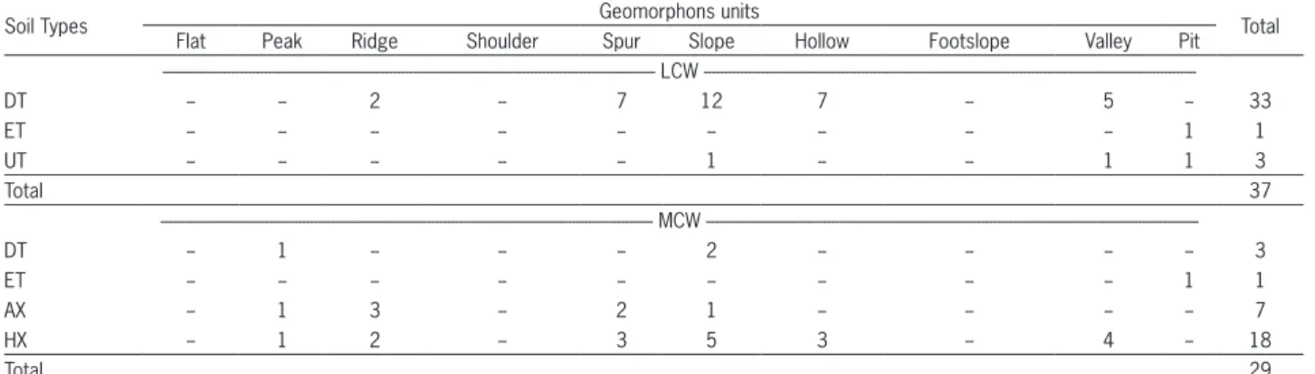
In order to clarify this hypothesis, observation points where soil morphological description and classi-fication had been performed were inserted in the Geo-morphons maps of highest correspondence with the soil types for the two watersheds and compared with the GUs where they were inserted (Table 3).
When analyzing Table 3, for LCW, it is evident that the majority of the DT is found in Slope GU, in
agree-ment with previous results. Furthermore, the unique point in an ET area was also in the same GU that the dominant one found by the calculations of areas on the polygon map (Pit). UT, in turn, has points occurring in Pit and Valley, which are characteristic of the landforms where this soil type is commonly found.
For MCW, most of the DT was found in Slope GU, in agreement with its incipient development, as it is as-sociated with more erosive places, while found in abun-dance in Valley in terms of area. However, ET, AX, and HX were found in the same previously observed GUs, Pit, Ridge, and Slope, respectively.
From this analysis, it was noticed that most soil types in the two watersheds (8 out of 11) were found in the same GU that predominated when analyzing the area of occurrence per soil type on the maps. It confirms that Geomorphons are capable of stratifying the land-scape in terms of soil type variability in these tropical conditions.
On the other hand, the only condition that dis-agreed (DT in MCW) indicates that this soil type may occur in different GUs. DT is a soil type that can be en-countered in different landscapes (Schaetzl and Ander-son, 2005), due to its classification by absence of defined characteristics, which means this soil class is highly variable in terms of properties, such as solum thickness, particle size distribution, color, drainage, slope gradient, and so forth.
To test soil property variability between the GUs, sand, silt, and clay contents at 0-20 cm depth were statis-tically evaluated (Table 4). Particle size distribution was selected for this test because, over time, it is considered a less variable soil property as it is little affected by land use and management practices, in contrast with soil or-ganic carbon, for example.
It is noticed that in LCW there was a statistical dif-ference between sand and clay contents in Valley and Pit GUs found in low and concave places, as compared to the other GUs relative to higher places in the landscape. Silt content did not differ between GUs, as they are gen-erally low in these weathered soils.
Table 3 − Number of observation points per soil class in each Geomorphons unit in the two watersheds in the study.
Soil Types Geomorphons units Total
Flat Peak Ridge Shoulder Spur Slope Hollow Footslope Valley Pit
LCW
---DT -- -- 2 -- 7 12 7 -- 5 -- 33
ET -- -- -- -- -- -- -- -- -- 1 1
UT -- -- -- -- -- 1 -- -- 1 1 3
Total 37
MCW
---DT -- 1 -- -- -- 2 -- -- -- -- 3
ET -- -- -- -- -- -- -- -- -- 1 1
AX -- 1 3 -- 2 1 -- -- -- -- 7
HX -- 1 2 -- 3 5 3 -- 4 -- 18
Total 29
On the other hand, for MCW, only the sand con-tent in Peak and Ridge GUs, the highest places in the landscape, differed from the others, probably due to partial clay removal by water. Also, clay content was very homogeneous in all parts of the watershed. These results may be an indicator of more weathered-leached soils in MCW than in LCW, which tends to diminish the soil property differences even in different land-forms under tropical conditions, along with different parent materials. The more developed the soils, the lower the variability of their properties (steady-state condition) (Birkeland, 1999). It seems soil particle size distribution in the two watersheds in tropical condi-tions has relatively low variability, and does not follow the difference in GUs and is contrary to the expected for temperate regions.
Bishop et al. (2012) raised the importance of the scientific validity of the results and the formal use of geo-morphological information generated nowadays, especial-ly in integrative sciences, such as Soil Science. Reliance has been placed on pattern recognition for segmentation and mapping, but whether or not such patterns represent phenomena, such as soil classes or properties, should be tested. In this sense, Qin et al. (2009) used a field study to relate slope position to A-horizon sand percentages through fuzzy logics. Likewise, in the current study, field work (soil survey and soil property sampling) with a GIS-based spatial statistic helped to understand the Geom-phorphons and its role in generating new capabilities in soil mapping under tropical conditions.
It is known that regional adaptations must be in-corporated in developed models to make them repre-sentative of soil variability in an area of interest. In this sense, Geomorphons can help to stratify the landscape into units that may have more homogeneity in terms of soil properties within themselves in an easy way, espe-cially in a first approach to allow not only for a better
understanding of soil occurrence in the landscape, but also for further refinement of soil maps. Further work should focus on adapting this tool to other Brazilian soil conditions in order to increase the details of this country's soil maps with reduced costs, since financial support for detailed soil mapping in Brazil is currently very scarce.
Conclusions
Geomorphons units have a strong relationship with soil types regardless pixel size and radius for Geo-morphons calculation in both watersheds.
When soil classification at observation points was compared with Geomorphons units, a high degree of correspondence was found with the results that took into account the soil type in soil maps with the dominant area per Geomorphons unit.
Particle size distribution does not vary according to Geomorphons units under the studied tropical condi-tions, due to the homogeneity found in these weathered-leached soils.
Acknowledgements
The authors thank CNPq (Brazilian National Council for Scientific and Technological Development), CAPES (Coordination for the Improvement of Higher Level Personnel) and FAPEMIG (Minas Gerais State Foundation for Research Support) for the financial sup-port for the development of this research.
References
Aquino, R.F.; Silva, M.L.N.; Freitas, D.A.F.; Curi, N.; Avanzi, J.C. 2013. Soil Losses from Typic Cambisols and Red Latosol as related to three erosive rainfall patterns. Revista Brasileira de Ciência do Solo 37: 213-220.
Ashtekar, J.M.; Owens, P.R.; Brown, R.A.; Winzeler, H.E.; Dorantes, M.; Libohova, Z.; Silva, M.; Castro, A. 2014. Digital mapping of soil properties and associated uncertainties in the Llanos Orientales, South America. p. 367-372. In: Arrouays, D.; McKenzie, N.; Hempel, J.; Forges, A.C.R.; McBratney, A., eds. GlobalSoilMap: Basis of global spatial soil informatio system. CRC Press, Boca Raton, FL, USA.
Beskow, S.; Mello, C.R.; Norton, L.D.; Curi, N.; Viola, M.R.; Avanzi, J.C. 2009. Soil erosion prediction in the Grande River Basin, Brazil using distributed modeling. Catena 79: 49-59. Birkeland, P. 1999. Soils and Geomorphology. Oxford University
Press, Oxford, England.
Bishop, M.P.; James, L.A.; Shroder Junior, J.F.; Walsh, S.J. 2012. Geospatial technologies and digital geomorphological mapping: concepts, issues and research. Geomorphology 137: 5-26. Bui, E.N. 2004. Soil survey as a knowledge system. Geoderma
120: 17-26.
Buol, S.W.; Southard, R.J.; Graham, R.C.; McDaniel, P.A. 2011. Soil Genesis and Classification. 6ed. Wiley-Blackwell, Ames, IA, USA.
Table 4 − Sand, silt, and clay content for the two studied watersheds. Geomorphon Units Sand (%) Silt (%) Clay (%)
--- LCW ---
Ridge 48.20 b 20.10 a 34.70 a
Spur 52.20 b 16.62 a 31.18 a
Slope 53.95 b 16.31 a 29.74 a
Hollow 52.00 b 17.71 a 30.28 a
Valley 57.14 a 18.48 a 24.38 b
Pit 58.00 a 14.25 a 27.75 b
MCW
---Peak 17.77 b 19.41 a 62.82 a
Ridge 18.84 b 19.88 a 61.27 a
Spur 21.06 a 18.41 a 60.23 a
Slope 21.81 a 18.96 a 59.23 a
Hollow 22.00 a 18.71 a 59.07 a
Valley 22.63 a 19.40 a 57.97 a
Pit 24.46 a 17.38 a 58.15 a
Cavazzi, S.; Corstanje, R.; Mayr, T.; Hannam, J.; Fealy, R. 2013. Are fine resolution digital elevation models always the best choice in digital soil mapping? Geoderma 195-196: 111-121. Chagas, C.S.; Curi, N.; Duarte, M.N.; Motta, P.E.F.; Lima, J.M.
1997. Orientation of layers of poor metapelitic rocks on genesis of Latosols (Oxisols) under cerrado vegetation. Pesquisa Agropecuária Brasileira 32: 539-548 (in Portuguese, with abstract in English).
Florinsky, I.V.; Kuryakova, G.A. 2000. Determination of grid size for digital terrain modelling in landscape investigations - exemplified by soil moisture distribution at a micro-scale. International Journal of Geographical Information Science 14: 15-832.
Hengl, T. 2006. Finding the right pixel size. Computers & Geosciences 32: 1283-1298.
Jasiewicz, J.; Stepinski, T.F. 2013. Geomorphons: a pattern recognition approach to classification and mapping of landforms. Geomorphology 182: 147-156.
Jenny, H. 1941. Factors of Soil Formation: A System of Quantitative Pedology. McGraw-Hill, New York, NY, USA.
McBratney, A.B.; Mendonça-Santos, M.L.; Minasny, B. 2003. On digital soil mapping. Geoderma 117: 3-52.
Mello, C.R.; Ávila, L.F.; Viola, M.R.; Nilton, C.; Norton, L.D. 2015. Assessing the climate change impacts on the rainfall erosivity throughout the twenty-first century in the Grande River Basim (GRB) headwaters, southeastern Brazil. Environmental Earth Sciences 73: 8683-8698.
Mendonça-Santos, M.L.; Santos, H.G. 2007. The state of the art of brazilian soil mapping and prospects for digital soil mapping. p. 39-54. In: Lagacherie, P.; McBratney, A.B.; Voltz, M., eds. Digital soil mapping: an introductory perspective. Elsevier, Amsterdam, Netherlands.
Menezes, M.D.; Silva, S.H.G.; Mello, C.R.; Owens, P.R.; Curi, N. 2014. Solum depth spatial prediction comparing conventional with knowledge-based digital soil mapping approaches. Scientia Agricola 71: 316-323.
Motta, P.E.F.; Curi, N.; Silva, M.L.N.; Marques, J.J.G.S.M.; Prado, N.J.S.; Fonseca, E.M.B. 2001. Detailed Soil Survey, Soil Erosion, Land Use and Agricultural Land Suitabitability of A Pilot Watershed in the Region under Influence of Camargos/Itutinga hydroelectric power plant-MG = Levantamento Pedológico Detalhado, Erosão dos Solos, Uso Atual e Aptidão Agrícola das Terras de Microbacia Piloto na Região sob Influência do Reservatório da Hidrelétrica de Itutinga/Camargos-MG. CEMIG, Belo Horizonte, MG, Brazil (in Portuguese).
Motta, P.E.M.; Curi, N.; Franzmeier, D.P. 2002 Relation of soils and geomorphic surfaces in the Brazilian cerrado. p. 13-32. In: Oliveira, P.S.; Marquis, R.J., eds. The cerrados of Brazil: ecology and natural history of a neotropical savanna. Columbia University Press, New York, NY, USA.
Qin, C.; Zhu, A.; Shi, X.; Li, B.; Zhou, C. 2009. Quantification of spatial gradation of slope positions. Geomorphology 110: 152-161.
Roecker, S.M.; Thompson, J.A. 2010. Scale effects on terrain attribute calculation and their use as environmental covariates for digital soil mapping. p. 55-66. In: Boettinger, J.L.; Howell, D.W.; Moore, A.C.; Hartemink, A.E.; Kienast-Brown, S., eds. Digital soil mapping: bridging research, environmental application and operation. Springer, Dordrecht, Netherlands. Schaetzl, R.J.; Anderson, S. 2005. Soils: Genesis and
Geomorphology. Cambridge University Press, Cambridge, UK. Staff, S.S. 1993. Soil Survey Manual. US Government Printing
Office, Washington, DC, USA.
Staff, S.S. 1999. Soil Taxonomy: A Basic System of Soil Classification for Making and Interpreting Soil Surveys, 2ed. USDA-SCS, Washington, DC, USA.