Analysis of surface soil moisture patterns in agricultural landscapes using empirical orthogonal functions

(1)

HESSD

6, 5565–5601, 2009

Analysis of surface soil moisture

patterns

W. Korres et al.

Title Page

Abstract Introduction

Conclusions References

Tables Figures

◭ ◮

Back Close

Full Screen / Esc

Printer-friendly Version

Interactive Discussion

Hydrol. Earth Syst. Sci. Discuss., 6, 5565–5601, 2009 www.hydrol-earth-syst-sci-discuss.net/6/5565/2009/ © Author(s) 2009. This work is distributed under the Creative Commons Attribution 3.0 License.

Hydrology and Earth System Sciences Discussions

Papers published inHydrology and Earth System Sciences Discussionsare under

open-access review for the journalHydrology and Earth System Sciences

Analysis of surface soil moisture patterns

in agricultural landscapes using empirical

orthogonal functions

W. Korres, C. N. Koyama, P. Fiener, and K. Schneider

Department of Geography, University of Cologne, Cologne, Germany

Received: 30 July 2009 – Accepted: 3 August 2009 – Published: 24 August 2009

Correspondence to: W. Korres (wolfgang.korres@uni-koeln.de)

(2)

HESSD

6, 5565–5601, 2009

patterns

W. Korres et al.

Title Page

Tables Figures

◭ ◮

Back Close

Full Screen / Esc

Abstract

Soil moisture is one of the fundamental variables in hydrology, meteorology and agri-culture. Nevertheless, its spatio-temporal patterns in agriculturally used landscapes

affected by multiple natural (rainfall, soil, topography etc.) and agronomic

(fertilisa-tion, soil management etc.) factors are often not well known. The aim of this study

5

is to determine the dominant factors governing the spatio-temporal patterns of surface soil moisture in a grassland and an arable land test site within the Rur catchment in Western Germany. Surface soil moisture (0–6 cm) has been measured in an approx.

50×50 m grid at 14 and 17 dates (May 2007 to November 2008) in both test sites.

To analyse spatio-temporal patterns of surface soil moisture, an Empirical Orthogonal

10

Function (EOF) analysis was applied and the results were correlated with parameters derived from topography, soil, vegetation and land management to connect the pattern to related factors and processes. For the grassland test site, the analysis results in one significant spatial structure (first EOF), which explains about 57.5% of the spatial variability connected to soil properties and topography. The weight of the first spatial

15

EOF is stronger on wet days. The highest temporal variability can be found in locations with a high percentage of soil organic carbon (SOC). For the arable land test site, the analysis yields two significant spatial structures, the first EOF, explaining 38.4% of the spatial variability, shows a highly significant correlation to soil properties, namely soil texture. The second EOF, explaining 28.3% of the spatial variability, is connected to

20

differences in land management. The soil moisture in the arable land test site varies

more during dry and wet periods on locations with low porosity.

1 Introduction

Soil moisture is one of the fundamental variables in hydrology, meteorology and agricul-ture as it plays a major role in partitioning energy, water and matter fluxes at the

bound-25

(3)

HESSD

6, 5565–5601, 2009

patterns

W. Korres et al.

Title Page

Tables Figures

◭ ◮

Back Close

Full Screen / Esc

influences the partitioning of precipitation into infiltration and runoff (Western et al.,

1999a) and it a_ffects the partitioning of incoming radiation into latent and sensible heat

due to the control of evaporation and transpiration. It has a strong impact on the re-sponse of stream discharge to rainfall events, it plays a significant role in producing

floods (Kitanidis and Bras, 1980) and a_ffects erosion from overland flow and the

gener-5

ation of gullies (Moore et al., 1988). More discharge and erosion have been observed, if areas with high soil moisture are well connected to the channels (Ntelekos et al., 2006). The spatio-temporal variation of soil moisture is also reflected in spatial pat-terns of plant growth and crop yield (Jaynes et al., 2003). For example, crop yield is highly sensitive to early season soil moisture conditions, especially during seed

germi-10

nation (Green and Erskine, 2004), thus emphasizing the importance of soil moisture seasonality.

Due to difficulties in measuring spatio-temporal patterns of soil moisture on larger

scales and owing to the importance of these patterns for many environmental

pro-cesses, great efforts were undertaken to derive spatially distributed soil moisture maps

15

from remote sensing and modelling (Oppelt et al., 1998; Owe and Van de Griend,

1998; Schneider, 2003). To build an adequate model, all relevant processes affecting

spatial and temporal soil moisture variability must be identified and addressed. How-ever, due to the multiple processes involved, spatio-temporal soil moisture patterns are very complex. In case of strong spatial variations in soil properties or a dominance of

20

vertical fluxes, such as evapotranspiration or infiltration, soil moisture patterns are con-trolled by local properties and processes (Grayson et al., 1997; Vachaud et al., 1985). If soil moisture is horizontally redistributed by lateral fluxes, non-local dependencies play a decisive role. Both, locally and non-locally controlled processes and their varying importance in time are essential for the determination of soil moisture patterns.

Haw-25

ley (1983) determines topography (relative elevation) as the most important driver of soil moisture in small agricultural watersheds. Even in watersheds with little slope, soil moisture values are consistently higher at the bottom of the slope. Vegetation tends to

(4)

HESSD

6, 5565–5601, 2009

patterns

W. Korres et al.

Title Page

Tables Figures

◭ ◮

Back Close

Full Screen / Esc

appears to be greater under wet conditions, minor variations in soil type seems to be insignificant. On 1.4 ha hillslope, Burt and Butcher (1985) detected the development of saturated areas in downhill, low slope and convergent locations, indicating lateral redistribution of soil water via saturated flow above impermeable bedrock. The cor-relation between Wetness Index (WI; Beven and Kirkby, 1979) and soil moisture was

5

generally better during wet conditions (Burt and Butcher, 1985). However, lateral water movement in unsaturated soils can also be observed and may reach the same order of magnitude as the vertical movement. This is caused by anisotropic permeability due to

different soil layers (Zaslavsky and Sinai, 1981). For the Tarrawarra grassland

catch-ment in south eastern Australia (Western et al., 1999a), the highest correlation between

10

soil moisture and topographic characteristics occurred on moderately wet conditions. This relationship deteriorates for dry and very wet (near saturation) conditions. The soil

moisture autocorrelation calculated for different dates generally showed longer

corre-lation length on dry dates, related to the greater spatial scale of evapotranspiration as the dominant driver. The shorter correlation length on wet days seems to be connected

15

to the smaller spatial scale of lateral redistribution (Western et al., 1998). Green and Erskine (2004) found no clear correlation length of soil moisture at the field scale for a semi-arid climate. Western et al. (2004) characterized the behaviour of soil moisture at several small humid and sub humid catchments and found typical correlation scales between 30 and 60 m. The comparison of the soil moisture correlation lengths with the

20

spatial correlation of terrain attributes indicates the important role of topography at one site and the variation of soil properties at other sites.

Empirical Orthogonal Function (EOF) analysis can be used to identify the dominant processes and essential parameters controlling soil moisture patterns. Since intro-duced to the analysis of geophysical fields by Lorenz (1956), EOF analysis is widely

25

(5)

HESSD

6, 5565–5601, 2009

patterns

W. Korres et al.

Title Page

Tables Figures

◭ ◮

Back Close

Full Screen / Esc

2007) to regional scales (Jawson and Niemann, 2007; Kim and Barros, 2002). The re-sult of this analysis is a small number of spatial structures (EOFs), explaining a high

percentage of variation of the dataset and temporal varying coefficients (ECs)

modulat-ing the influence of these spatial structures in time. With a correlation analysis, these underlying (stable) patterns of soil moisture variations can be connected to parameters

5

derived from topography, soil, vegetation, land management and meteorology. The main objectives of this study are: (i) to analyse the spatio-temporal surface soil mois-ture patterns in a grassland and an arable land test site by applying an EOF analysis and (ii) to determine the potential of this method to derive the dominating parameters and the underlying processes governing these patterns.

10

2 Test sites

Field measurements were carried out in the framework of the SFB/TR32 project in a grassland test site in Rollesbroich and an arable land test site in Selhausen, both

located west of Cologne. The grassland site (50◦₃₇′₂₅′′_N/6◦₁₈′₁₆′′_{E) covers an area}

of approximately 20 ha with nine fields of extensively used grassland (Fig. 1), typical

15

for the rolling topography of the Eifel. Slopes range from 0 to 10◦, while altitude ranges

from 474 to 518 m a.s.l. Measurements taken at a meteorological station 9 km to the

west (altitude 505 m) of the test site yield an annual mean air temperature of 7.7◦C and

an average annual precipitation of 1033 mm without a clear seasonality. The dominant soils are (gleyic) Cambisol, Stagnosol and Cambisol-Stagnosol. Due to the dense root

20

network of the grass cover, the amount of soil organic matter (SOM) in the topsoil

(<5 cm) is greater than 8% by weight. Hence low bulk densities (0.57 to 0.83 g cm−3)

prevail, with smallest values measured in the low lying northern part of the test site with dominating gleyic soils. The grassland vegetation is dominated by a ryegrass society, particularly perennial ryegrass (Lolium perenne) and smooth meadow grass

25

(Poa pratensis).

(6)

HESSD

6, 5565–5601, 2009

patterns

W. Korres et al.

Title Page

Tables Figures

◭ ◮

Back Close

Full Screen / Esc

and represents an intensively used agricultural area, where crops are grown on slight

slopes (0–4◦_{). The altitude ranges from 102 to 110 m a.s.l.. A mean annual air}

tem-perature of 9.8◦C and an average precipitation of 690 mm with slightly higher values

occurring in June and July were measured at a meteorological station 4.5 km to the north-west (altitude 90 m). Main soils are (gleyic) Cambisol and (gleyic) Luvisol with

5

a high amount of coarse alluvial deposits on a former river terrace in the eastern part. The land cover types during the measurement period were sugar beet (beta vulgaris), wheat (triticum aestivum), rye (secale cereale), oilseed radish (raphanus sativus oleiformes) and fallow.

3 Field Measurements

10

3.1 Grassland test site

Surface soil moisture measurements for the topsoil layer (0–6 cm) were performed on

a 50×50 m grid (Fig. 1). The measurement locations were slightly adjusted

accord-ing to local conditions such as field boundaries. While the typical distance to the next measuring location was 50 m, the minimum distance was 20 m and ranged up to 60 m.

15

Measurements were taken for 14 campaigns from May 2007 to November 2008. In order to provide validation measurements for remotely sensed surface soil moisture maps, the days of measurement were selected to match the overpass of ENVISAT. Measurements were taken at 41 to 96 locations. To provide representative values, each measurement location is represented by the average of six measurements

car-20

ried out in a radius of 10 cm. Soil moisture was measured with handheld FDR probes (Delta-T Devices Ltd., Cambridge, UK). The probes were calibrated individually in the laboratory using a mixture of water and glass beads to provide well defined water

con-tent. For mineral soils the, calibrated FDR probes yield a precision of+/−1 Vol.-%. To

evaluate the influence of soil texture and soil organic carbon (SOC) on the surface soil

25

(7)

HESSD

6, 5565–5601, 2009

patterns

W. Korres et al.

Title Page

Tables Figures

◭ ◮

Back Close

Full Screen / Esc

at every sampling location. Carbon content and soil texture were determined using mid-infrared-spectroscopy (Bornemann et al., 2008). The results from spectroscopy analysis were calibrated to carbon content using samples analysed with a CNS Ele-mentar Analysator (EleEle-mentar, Germany). In addition, bulk density and soil organic matter (SOM) were measured for the topsoil of four selected locations in the northern

5

part of the test site. These measurements were made to validate the extremely high surface soil moisture values (up to 75 Vol.-%) measured, especially in field F2. These

bulk density measurements yielded values of 0.69, 0.57, 0.78 and 0.83 g/cm3, thus

providing evidence for a very high total porosity in these locations.

3.2 Arable land test site

10

Similarly to the grassland test site, surface soil moisture (<6 cm) was measured in the

arable land test site on a grid of approx. 50×50 m (Fig. 1). Also here, the locations

were adjusted according to local conditions and field boundaries. Measurements were taken for 17 days of ENVISAT overpasses between May 2007 and November 2008 at 44 to 118 locations. Soil information was taken from a high resolution soil map

15

(Bodenkarte 1:50 000, Geologischer Dienst, North-Rhine-Westphalia). A terrace slope

with an elevation difference of about 2–3 m cuts through the test site. Tillage effects

at the edge of the terrace result in a high percentage of stones at the surface in the vicinity of the terrace slope. The upper terrace plain has a high stone content, while the lower plain generally shows a lower stone content. The surface stone cover was

20

mapped by visually estimating the surface stone coverage at each measuring location.

Three replicates were used, each covering a 40×40 cm sample area. This stone cover

(8)

HESSD

6, 5565–5601, 2009

patterns

W. Korres et al.

Title Page

Tables Figures

◭ ◮

Back Close

Full Screen / Esc

4 Methods

4.1 EOF analysis

Empirical Orthogonal Functions (EOF) analysis is one of the best known data analysis

techniques and a well established method of multivariate data analysis (Jolliffe, 2002).

The EOF analysis, also known as principal component analysis, decomposes the

ob-5

served variability of a dataset into a set of orthogonal spatial patterns (EOFs) and a set

of time series called expansion coefficients (ECs). The terminology used here follows

Perry and Niemann (2007). Other sources refer to the EOFs as “principle component loadings”, “loadings”, “scores” or “principle components”, ECs are referred to as “EOF

time series”, “Principle Component time series” or “Pattern Coefficients”.

10

Measurements, taken at location x_i(i= 1, . . . p) and at time tj (j=1, . . . n), are

ar-ranged into a matrixD (n by p: n sampling times and p sampling locations), in a so

called S-mode. Each row of the matrix represents the measurements at one point in time at all locations and each column represents a time series of measurements for

a given location. To analyse the spatial variability of the data, a matrixFis computed

15

from the matrixDby subtracting the average of each row of the data matrixD(average

soil moisture for a given observation time over all measurements locations). Analo-gously, to analyse the temporal variability, the average of each column is subtracted for

matrixD(average soil moisture for a given location for all measurements conducted at

that location). In the next step, the covariance matrixR(pbyp) of the data matrixFis

20

calculated:

R= 1

N₋1F

t_F ₍₁₎

where the subscriptt indicates a transposed matrix andN is the number of

observa-tions.

Ris diagonalized to find the eigenvectors and eigenvalues:

25

(9)

HESSD

6, 5565–5601, 2009

patterns

W. Korres et al.

Title Page

Tables Figures

◭ ◮

Back Close

Full Screen / Esc

where Λ (p by p) is a diagonal matrix containing the eigenvalues λ_i of R and C (p

by p) contains the eigenvectors ci of R in the column vectors, corresponding to the

eigenvaluesλ_i. For more details on the procedure see Jolliffe (2002), Hannachi (2007)

or Preisendorfer (1988).

This procedure rotates the original coordinate axes in a multidimensional space to

5

align the data along a new set of orthogonal axes in the direction of the largest variance. Thus, the first axis or eigenvector is oriented in the direction that explains of the largest variance. The subsequent axes are constrained to be orthogonal to the axes computed before and explain consecutively the largest part of the remaining covariance. The

eigenvectors c_i _{in the columns of the matrix} _C _{are the EOFs. The EOFs represent}

10

patterns or standing oscillations that are invariant in time. To analyse, how the EOFs

evolve in time, the expansion coefficients (ECs) associated with each EOF is calculated

by projecting the matrixFonto the matrixC:

A₌FC (3)

where the matrixAcontains the expansion coefficientsa_i in the column vectors.

15

The EOF analysis producesp(p₌sampling locations) EOF/EC pairs, but only the

minimum of (n;p) (n ₌ sampling times) has an eigenvalue greater than zero and is

therefore meaningful. Usually the EOFs and ECs are rearranged in descending order due to their eigenvalues, so that the first EOF (EOF1) is associated with the largest

eigenvalue. The fraction of variance explained (EV) by each EOF can be found by

20

dividing the associatedλ_i by the sum of all eigenvalues (the trace ofΛ):

E V_i ₌ λi

p

P

i=1

λ_i

(4)

Following Bj ¨ornsson and Venegas (1997) and Hannachi et al. (2007), the EOFs and

(10)

HESSD

6, 5565–5601, 2009

patterns

W. Korres et al.

Title Page

Tables Figures

◭ ◮

Back Close

Full Screen / Esc

computing the covariance matrix and solving the eigenvalue problem. This decompo-sition by SVD provides a compact representation, because it drops unnecessary zero singular values (equivalent to zero eigenvalues).

4.2 Selection rules for EOFs

In principle, after decomposition, the EOFs and ECs can be used to reconstruct the full

5

variability of the dataset by selecting all EOF/EC pairs. However, to approximate and compress a dataset, only the first few EOF and EC pairs, which explain the largest frac-tion of variance, are usually selected. This results in a reducfrac-tion of dimensionality. By truncating the system, a “cleaner” version of the dataset is constructed, because ran-dom noise contained in the higher order EOF’s is eliminated (Bj ¨ornsson and Venegas,

10

1997; Preisendorfer, 1988). In practice, this truncation is often achieved by selecting a threshold for the overall explained variance (e.g. 80%) and choosing the set of lead-ing EOFs that cumulatively explain at least this amount of variance. A prerequisite for

the physical interpretation of single EOFs is that the EOFs are significantly different

from each other. The linear combination of two EOFs, which are not significantly diff

er-15

ent and thus degraded, may be based upon the same underlying physical processes. Thus, any linear combination of patterns based on degraded EOFs is as significant as each one of them (Hannachi et al., 2007).

To estimate the correct number of significant patterns (EOFs) for the subsequent physical interpretation, two selection rules are applied. One rule utilizes a measure of

20

uncertainty for the eigenvalues and is summarized by the rule of thumb (North et al.,

1982) defining the typical error (∆) of eigenvalues:

∆(λ_i)≈λi

r 2

s (5)

(11)

HESSD

6, 5565–5601, 2009

patterns

W. Korres et al.

Title Page

Tables Figures

◭ ◮

Back Close

Full Screen / Esc

The 95% confidence interval (CI₉₅) for each eigenvalue is then given by:

CI

95(λi)≈λi(1±

r 2

s) (6)

The EOFs are considered to be significant if the 95% confidence intervals of the neigh-bouring eigenvalues are not overlapping with another.

An additional rule is to use Monte Carlo simulations to estimate the uncertainties of

5

the eigenvalues (Rule N; Preisendorfer, 1988). The eigenvalues of the measured data set have to be significantly higher than the eigenvalues of a random dataset. To test this, one thousand realisations of normally distributed surrogate data between zero

and one (white noise) in the dimension of the matrix of the original dataset (n by p)

are formed and analysed by the EOF analysis. From the results of these one

thou-10

sand realisations, the upper 95% confidence interval of the eigenvalues is calculated and taken as the limit for the significance of the eigenvalues of the measured dataset. Another calculation with randomized measured values instead of normally distributed surrogate data resulted in the same number of significant EOFs and is not additionally presented here.

15

Both selection rules are used in our data analysis to determine the number of

signifi-cant EOF/EC pairs. Both require knowledge of the number of independent samples (s).

In Eq. (6), the number of independent samples is used directly to estimate the errors of the eigenvalues and in the Monte Carlo analysis, the dimensions of the surrogate

data matrix are changed from (nbyp: nsampling times andpsampling locations) to

20

(nby s), resulting in a higher limit for the first few EOFs to be considered significant.

To evaluate the spatial interdependencies between the measuring points, a spatial au-tocorrelation analysis was performed, calculating Moran’s I statistic for a number of distance classes. 25 distance classes, each containing 183 data pairs for each day of measurement, were calculated for the grassland. For the arable land test site, 30

25

(12)

HESSD

6, 5565–5601, 2009

patterns

W. Korres et al.

Title Page

Tables Figures

◭ ◮

Back Close

Full Screen / Esc

to be autocorrelated. The EOF analysis requires independent samples. Thus, to ac-count for the influence of spatial autocorrelation on the evaluation of significant EOFs, the number of sampling locations is reduced by these percentages of autocorrelated distance pairs, resulting in 81 and 107 independent spatial sampling locations in the grassland test site and the arable land test site, respectively. For the temporal analysis

5

we assume that the dates of each measuring campaign are independent and choose the maximum possible degrees of freedom in the time domain.

4.3 Correlation analysis

The aim of the EOF analysis is to identify stable spatial and temporal patterns. To esti-mate the dominant drivers governing the surface soil moisture patterns, the EOFs were

10

correlated with parameters derived from topographical, soil, vegetation, land manage-ment and meteorological data.

The EOFs may only be correlated with parameters that are invariant in time. The temporal development of biomass may explain, to some degree, the soil moisture pat-terns at a given day due to growth, cutting or grazing for instance, but it does not

15

provide a temporally invariant signal and is therefore not suitable to explain the EOF patterns.

The parameters used in this correlation analysis are associated with parameters de-termining horizontal (lateral) (e.g. elevation, flow accumulation, curvature etc.) and vertical (e.g. field capacity, soil texture, SOC etc.) flow of water. Elevation, multiple

20

flow accumulation (e.g. specific drainage area), natural log of the multiple flow

accu-mulation, slope, slope−1, horizontal curvature, vertical curvature and Wetness Index

are computed from a 10 m DEM (Sci Lands, 2008) with ArcGis 9.2 (ESRI, USA). Soil type data in the grassland test site was derived from the 1:5000 soil map (Geologis-cher Dienst, North-Rhine-Westphalia) and is particularly used to delineate an gleyic

25

(13)

HESSD

6, 5565–5601, 2009

patterns

W. Korres et al.

Title Page

Tables Figures

◭ ◮

Back Close

Full Screen / Esc

silt, sand and SOC in the grassland test site were determined as described in Sect. 3. Topographic parameters such as Wetness Index, Flow Accumulation, Slope and Cur-vature were not computed for the arable land test site, since in this predominantly flat

area, the flow path is affected by features such as field boundaries and tillage tracks

within the field rather than the slope given in the DEM. Several parameters used to

5

explain the EOFs are interrelated (e.g. field capacity, % sand, % silt and % clay) and thus point to the same hydrological process.

5 Results

5.1 Analysis of field measurements

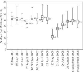
Both test sites show a large range of different soil moisture conditions (Figs. 2, 3),

10

ranging from very dry conditions (22.2 Vol.-% in the grassland test site, and 19.5 Vol.-% in the arable land test site) to very wet conditions (54.3 Vol.-%, 32.5 Vol.-%, resp.). The average soil moisture over all measurements generally indicates higher values (46.5 Vol.-%) for the grassland site as compared to the arable land test site (26.6 Vol.-%). The spatial variability of the soil moisture on each day of measurement is comparable

15

in both test sites. The average standard deviation of the soil moisture over all days of measurement in the grassland test site is 4.5 Vol.-% (Min.: 3.2 Vol.-%, Max.: 5.8

Vol.-%, coefficient of variance (CV): 9.6%) and in the arable test site, it is 3.8 Vol.-%

(Min.: 2.3 Vol.-%, Max.: 6.3 Vol.-%), CV: 14.2%). Due to the higher soil moisture status in the grassland test site, the range of the average soil moisture in the grassland test

20

site (32.1 %) exceeds the respective range in the arable land test site (13.1

Vol.-%) These differences are due to higher precipitation, the higher soil porosity and the

higher amount of soil organic carbon content (SOC) in the topsoil of the grassland test site. Extremely high surface soil moistures were particularly measured in field F2 in the grassland test site. Due to the high organic content, the maximum porosity reached

25

(14)

HESSD

6, 5565–5601, 2009

patterns

W. Korres et al.

Title Page

Tables Figures

◭ ◮

Back Close

Full Screen / Esc

soil moisture reached 40%. The length of the whiskers in Fig. 2 indicates a large spatial variability of the surface soil moisture in the grassland test site. The average range of the soil moisture values measured in the grassland test site is 25.3 Vol.-% (Min.: 14.3 Vol.-%, Max.: 36.1 Vol.-%) and 18.4 Vol.-% (Min.: 9.1 Vol.-%, Max.: 25.9 Vol.-%) in the arable land test site. The measurements of the 14 days of measurement in the

5

grassland test site and the 17 in the arable test site accumulate to a total number of 17 124 FDR-measurements. The EOF analysis requires a continuous data set without missing data. Thus only 8 of the 14 measurement days from the grassland test site and 10 of the 17 measuring days from the arable land test site were used for the subsequent analysis.

10

5.2 EOF-Analysis

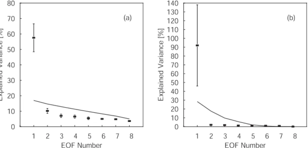
The analysis of the spatial patterns in the grassland test site yields a set of 8 EOF/EC pairs. EOFs calculated for analysing spatial patterns are called henceforth spatial EOFs, analogously EOFs calculated to investigate temporal patterns are referred to as temporal EOFs. The spatial EOF1 of the grassland test site explains 57.5% of the

15

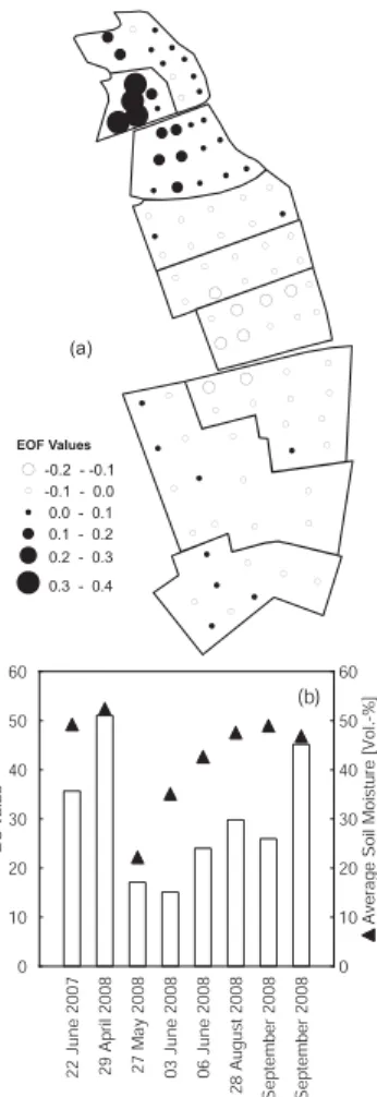
spatial variance of the dataset, while EOF2 explains only 10.2% (Fig. 4a). The 95% confidence limit of the Monte Carlo simulation exceeds the explained variance of EOF2 to EOF8. Also, the 95% confidence interval of EOF1 does not overlap with the neigh-bouring EOFs. As a result, the first EOF is significant. The pattern of the spatial EOF1 (Fig. 5a) shows high values with positive signs. This indicates higher than average soil

20

moisture values in the northern part (fields F1, F2 an F3), which is in the valley section of the test site. Highest positive values can be found in field F2. Minimum values with negative signs are located in the central part of the test site (field F6). The EOF values

increase slightly towards the southern part. The associated expansion coefficient

(spa-tial EC1, Fig. 5b) shows a maximum value on 29 April 2008 and a minimum value on

25

3 June 2008. This maximum EC1 values coincides with the high average soil moisture values on these measuring dates, while the low EC values indicate dry conditions.

(15)

HESSD

6, 5565–5601, 2009

patterns

W. Korres et al.

Title Page

Tables Figures

◭ ◮

Back Close

Full Screen / Esc

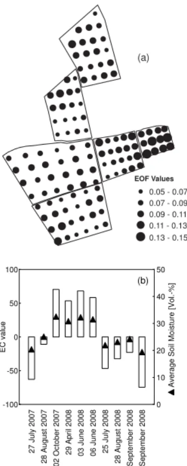
EOF/EC pairs. The spatial EOF1 explains 38.4% and EOF2 28.3% of the spatial vari-ability of the dataset (Fig. 6a). Only these first two EOFs satisfy the significance re-quirements, because the 95% confidence intervals of their eigenvalues neither over-lap with neighbouring confidence intervals nor with the 95% confidence interval of the eigenvalues of the Monte Carlo simulation. The spatial EOF1 (Fig. 7a) shows the

low-5

est negative values in the eastern part of the test site and an irregular and patchy pattern with higher values in the rest of the test site. The EOF2 (Fig. 7b) shows a two peaked distribution with high positive values on some fields contrasted by low negative values on other fields with an abrupt change of the EOF values typically at the field boundaries. The values of the EC1 (Fig. 7c), which express the weight of the EOF1

10

on the di_fferent dates, are positive on all dates and reach a maximum value on 27 July

2007 and a minimum value on 24 April 2008. The values of the EC2 (Fig. 7d) show a minimum value with a negative sign on 19 September 2008 and a maximum and positive value on 27 July 2007. Thus, the influence of the EOF1 varies only gradually during the dates of measurements, while the EOF2 reverses its influence in an annual

15

cycle.

Both analyses, for the grassland and the arable land test site, resulted in only one significant temporal EOF/EC pair (Figs. 4b and 6b). The temporal EOF1 of the grass-land test site explains 92% of the temporal variance and all values are positive. It shows a pattern similar to the spatial EOF1. Smaller and negative values occur in

20

the northern part of the test site. However, the pattern is more irregular and patchy (Fig. 8a) as compared to the spatial EOF. The temporal EC1 has a maximum value on 27 May 2008 and a minimum value on 29 April 2008 (Fig. 8b). The temporal EOF1 of the arable land test site explains about 72.5% of the temporal anomalies of the data set (Fig. 6b) and has all positive values with maximum values in field F3 in the eastern

25

part of the test site (Fig. 9a). The associated EC1 has the highest positive value on 2 October 2007 and the lowest negative value on 10 September 2008 (Fig. 9b).

(16)

HESSD

6, 5565–5601, 2009

patterns

W. Korres et al.

Title Page

Tables Figures

◭ ◮

Back Close

Full Screen / Esc

values, because the soil moisture variability explained by this EOF/EC pair (anomalies) is computed by multiplying EOF and EC.

5.3 Correlation analysis

The spatial patterns computed from the EOF analysis were correlated with different

parameters for the grassland (Table 1) and the arable land test sites (Table 2). These

5

parameters were derived from topography, soil, vegetation and land management data and allow relating the patterns found in the EOF analysis to driving processes. Only significant correlations of the EOF patterns with the parameters are presented in the tables. The spatial patterns found for the grassland test site show the highest Pearson

correlation coefficient with elevation and the soil property gleyic/non gleyic. By

distin-10

guishing between gleyic and non gleyic soils, an ordinal scale is defined for use in the correlation analysis. The highest correlation for the temporal pattern is found with SOC, percentage of sand in the topsoil (0–10 cm) and soil type. In the arable land test site the first spatial pattern is highly correlated with elevation and soil parameters, particu-larly the percentage of stone cover and field capacity (Table 2). The correlations of the

15

parameters with the temporal EOF1 pattern are smaller but also highly significant. The second spatial pattern (EOF2) cannot be correlated with any of the tested parameters. The temporal course of the EC1 values of the spatial analysis in both test sites show a

high correlation coefficient with the average soil moisture (R ₌0.73 for grassland,R ₌

−0.71 for arable land). The temporal course of the EC1 patterns for the temporal

anal-20

ysis shows a perfect correlation to the mean soil moisture for both test sites (Table 3).

The different signs of the Pearson correlation coefficients are due to the different signs

(17)

HESSD

6, 5565–5601, 2009

patterns

W. Korres et al.

Title Page

Tables Figures

◭ ◮

Back Close

Full Screen / Esc

6 Discussion

6.1 Spatial analysis

The analysis performed on the spatial variability in the grassland test site shows that the main soil moisture pattern (spatial EOF1) is strongly related to soil properties and explains about 57.5% of the spatial soil moisture variation. The highly significant

cor-5

relations with the soil property gleyic/non gleyic (R ₌ 0.7), soil texture (e.g. % sand

0–10 cm: R ₌₋0.42), and SOC (R ₌0.47 for 0–10 cm and R ₌ 0.37 for 10–30 cm)

indicate a clear connection to infiltration (vertical process). The impermeable soil layer of a Stagnosol resulted in a higher amount of organic matter and also in a very low bulk density in the topsoil at these points. The pattern also has a strong resemblance

10

to the catchment topography. The strong correlations to parameters such as elevation

(R ₌₋0.57), natural logarithm of flow accumulation (R ₌0.45), slope (R ₌0.46) and

Wetness Index (R ₌0.34) indicate that the spatial pattern is related to landscape

po-sition, which is affects two processes: the position within the landscape determines

(i) the redistribution of water through surface runoff and subsurface drainage and (ii)

15

the amount of solar radiation received at this position, affects the evapotranspiration

amount.

Perry and Niemann (2007) applied an EOF analysis to the widely studied soil mois-ture dataset of 459 locations on 13 dates from the 10.5 ha Tarrawarra grassland catch-ment (Western and Grayson, 1998; Western et al., 1998, 2001, 1999b, 1999a). The

20

first EOF in their study explained 55% of the spatial variability of soil moisture. Similar to our results a clear dependence on hillslope and valley topography was found and most prominent during wet periods. Our EOF analysis yielded one significant spa-tial EOF explaining 57.5% of the variance. Due to the smaller size of our dataset the spatial EOF2 (10% explained variance) is statistically not significant, whereas the

sec-25

(18)

HESSD

6, 5565–5601, 2009

patterns

W. Korres et al.

Title Page

Tables Figures

◭ ◮

Back Close

Full Screen / Esc

variability of soil moisture and the relative roles of various affecting factors with the

data of the SGP97 Little Washita field site (Famiglietti et al., 1999). Their first EOF accounts for over 70% of the variability for interstorm periods and over 60% for the whole dataset. The most important factors here are topography related to a decreas-ing role after rainfall stops and an increasdecreas-ing role of soil- and land-use-related factors.

5

Jawson and Niemann (2007) decomposed remotely sensed soil moisture data from the SGP97 field campaign with an EOF analysis and found a single pattern explaining 61% of the observed spatial variability. The most related physical characteristic to the EOF pattern seemed to be soil texture (percent sand and percent clay). In contrast to the findings of Yoo and Kim (2004), topographic characteristics were relatively

unim-10

portant and diminished on drier conditions. Jawson and Niemann (2007) assumed that this contrast may have occurred, because topographic characteristics influenced soil moisture largely through lateral flows, which were not easily observed on the scale of this study.

In conclusion, our study agrees with the previously mentioned studies in that about

15

55% to 70% of surface soil moisture variability can be explained by stable patterns and is correlated to topography and soil parameters. On the other hand, our result for the grassland test site indicates that 42.5% of the spatial variability varies in time and can therefore not be explained by a stable spatial pattern. This portion of the overall

variance is mainly due to differences in management (grazing, cutting and fertilizing)

20

of the different fields. Also random noise due to measurement errors contributed to

the unexplained variance. In the EOF analysis of spatial patterns, the impact of

tem-porally variable factors, which do not affect the whole area uniformly, results in noise;

decreases the amount of the variance explained by the significant EOFs or decreases

the number of significant EOFs. In addition, a difficulty in interpreting the results for

25

the grassland test site is that the function and location of old drainage pipes on field F6 is not exactly known. While the low values of field F6 might indicate that the drainage

tiles are still functioning, a clear relationship with this effect cannot be established. The

(19)

HESSD

6, 5565–5601, 2009

patterns

W. Korres et al.

Title Page

Tables Figures

◭ ◮

Back Close

Full Screen / Esc

tiles are functional.

The spatial EC1 is positively correlated with the average soil moisture of the mea-suring days, meaning that on wet days the pattern of the EOF1 has a stronger influ-ence on the soil moisture values than on drier days. As expected, during wet periods,

lateral redistribution of water over longer distances is possible and the e_ffect of the

5

impermeable soil layer of the soil type (Stagnosol) upon surface soil moisture is more pronounced. This leads, in combination with the higher amount of organic matter and lower bulk density in the Stagnosol area of the test site, to very high topsoil moisture values (up to 75 Vol.-%). The impact of the Stagnosols decreases as the soil dries with increasing evapotranspiration. Prior findings of Perry and Niemann (2007),

indi-10

cating a pronounced decrease of the weight of the spatial EOF1 pattern on very dry and very wet conditions, cannot be confirmed by our dataset. Potential causes of this discrepancy might be that we had only few measurements under dry conditions. Also, the first EOF in the Tarrawarra test site is primarily related to landscape position and the associated lateral redistribution of water and subordinately to evapotranspiration,

15

while ours is mainly related to soil properties and only secondarily related to landscape position.

Most previous studies working on a comparable spatial scale to our study focussed on test sites with little management impacts. Our study also looked at spatial anoma-lies in an arable land test site. Our results show, that the first spatial EOF in the arable

20

land test site is still related to soil properties, namely surface stone cover (R ₌₋0.79)

and field capacity (R₌0.75) and explains 38.4% of the variance. However, the second

EOF indicates effects originating from different tillage practices of the different fields.

The spatial patterns of the first EOF can be explained from the effects of an old river

terrace which crops out in the eastern part of the test site approximately at elevation

25

107 m (see Fig. 1) and causes a high amount of coarse alluvial deposits in the adjacent fields (F1/3/4), especially on field F3. Both parameters, stone cover and field

capac-ity, underline the importance of spatial differences of soil properties in relation to soil

(20)

HESSD

6, 5565–5601, 2009

patterns

W. Korres et al.

Title Page

Tables Figures

◭ ◮

Back Close

Full Screen / Esc

be judged as an artefact from the cross correlation of the presence of outcrop of the old river terrace and its position in the elevation gradient. The correlation between the

spatial EC1 and the average soil moisture (R ₌0.71) shows that the influence of the

EOF1 pattern associated with soil properties is more pronounced on dry dates. Due to the lower porosity in the eastern part of the test site, soil moisture decreases more

5

rapidly after precipitation.

The spatial EOF2 shows no significant correlation with any of the tested parameters. However, the variation of the spatial EOF2 values is quite small within the individual

fields (coefficient of variation (CV) between−5.2 and 0.6) while it is pronounced

be-tween different fields (CV:−43.5), which indicates that the EOF2 pattern is dominated

10

by tillage e_ffects. The importance of tillage e_ffects upon soil moisture can be shown

exemplarily for soil moisture dates with similar patterns to the spatial EOF2 values (27 July 2007 between the adjacent fields F5 and F6; 19 September 2008 between the adjacent fields F1 and F2). On both dates, the wetter field of the two is harvested while the much drier field is also ploughed the week before the measurements. Because of

15

the higher porosity after ploughing, soil moisture decreased inducing a steep gradient at the field boundaries. This pattern can be fully reversed after a precipitation event, if the larger pore volume of the ploughed field is filled with water. The highest pos-itive and negative values of the spatial EC2 can be found on days with low average soil moisture, when some field are ploughed shortly before the measurements (27 July

20

2007, 16 September 2008 and 19 September 2008). High values are found on days with low average soil moisture values where some fields are harvested or drilled (28 August 2007 and 28 August 2008). Low spatial EC2 values can be found on days with high average soil moisture values (even when some fields are ploughed) or on days with comparable vegetation cover in all fields (even when the average soil moisture is

25

low). Due to multiple vegetation periods covered in our multi-annual dataset, there is

no spatial stability with regards to land management effects. This is reflected in the

(21)

HESSD

6, 5565–5601, 2009

patterns

W. Korres et al.

Title Page

Tables Figures

◭ ◮

Back Close

Full Screen / Esc

management by tillage (increase of pore volume after ploughing, differences in

evapo-ration) and di_fferent crop rotation or vegetation heights (resulting in di_fferences of

tran-spiration). These results from the spatial analysis show that it is possible to apply EOF analyses on managed agricultural fields or regions. The structure of our dataset with reversing management patterns in the two consecutive years of measurements makes

5

it possible to detect not only the stable pattern (connected with soil parameters), but

also the non stable pattern of different land management options on the different fields.

6.2 Temporal analysis

The temporal analysis identifies locations with great temporal variability. These loca-tions are identified by high absolute numbers in Fig. 8a. Both temporal EC1s have a

10

perfect correlation with the average soil moisture on the days of the measurements, substantiating the control of these patterns by wet and dry periods. One dominant mode of temporal variability in each test site with all negative EOF1 values in the grassland test site and all positive EOF1 values in the arable land test site indicates a consistent reaction of the soil moisture values on dry and wet periods in the same

15

direction on each test site. Both test sites are small enough to assume homogeneous precipitation across the fields over the time of measurements. The comparatively high value of explained variance (13.1%) of the temporal EOF2 in the arable land test site might indicate the influence of land management. The temporal EOF1 in the grassland test site explains 92% of the temporal variance. It is related to soil properties (e.g. %

20

SOC:R₌₋0.44; Soil Type: R₌₋0.34; % Sand: R₌0.33) and catchment topography

(e.g. Elevation: R ₌ 0.27). Therefore, the highest soil moisture variability during dry

and wet periods can be found in the lower parts of the test site at locations with a high percentage of SOC and SOM due to the Stagnosol soils in this area. In the arable land test site, the points with the highest temporal EOF1 values are correlated with surface

25

stone cover (R₌0.48) and field capacity (R₌₋0.41), implying that soil moisture varies

(22)

HESSD

6, 5565–5601, 2009

patterns

W. Korres et al.

Title Page

Tables Figures

◭ ◮

Back Close

Full Screen / Esc

7 Conclusions

Our study shows that Empirical Orthogonal Function analysis can be used to detect the spatial and temporal patterns of surface soil moisture, in order to capture the main dynamical behaviour of the system. A subsequent correlation analysis provides an avenue to explain the spatial and temporal patterns based upon dominant factors and

5

processes. In the grassland test site (Rollesbroich), one significant spatial pattern, explaining 57.5% of the spatial soil moisture variability, was found. This pattern is related to soil properties (soil type) and topography. Its dominance is largest during or shortly after wet periods, because under wet conditions, the lateral redistribution

of water and the varying infiltration by di_fferent soil types becomes more important.

10

Another significant spatial pattern accounting for the differences in land management

(grazing, cutting, fertilizing) could not be identified for the grassland site. The highest soil moisture variability was found in the lower parts of the test site at locations with a high percentage of SOC and influenced by the soil type in that area.

In the arable land test site (Selhausen), two significant patterns controlling the major

15

part of the spatial variability were determined. The first pattern (spatial EOF1), ac-counting for 38.4% of the variance, is strongly related to soil properties (surface stone cover and field capacity). The impact of this pattern is more pronounced during dry

periods, indicating a compensating e_ffect of precipitation. The second pattern (spatial

EOF2) explains 28.3% of the variance and can be assigned to different land

manage-20

ment patterns, influencing soil properties and evaporation by tillage and transpiration,

due to di_fferent crops and di_fferent dates of sowing and fertilization. More than 66%

of the spatial variability of surface soil moisture in the Selhausen test site can be ex-plained by these two patterns associated with soil properties and land management. The highest temporal variability of soil moisture during the dry and wet periods can be

25

found on locations with low porosity.

Large portions of the overall variance of the soil moisture can be explained by

(23)

HESSD

6, 5565–5601, 2009

patterns

W. Korres et al.

Title Page

Tables Figures

◭ ◮

Back Close

Full Screen / Esc

EOF analysis provides an objective method to identify the dominant drivers of spatio-temporal patterns in soil moisture data sets and to quantifying the amount of influ-ence on the soil moisture patterns. Thus, knowing the underlying spatial patterns and the explained variance, it is possible to estimate soil moisture patterns based upon knowledge of the areal average soil moisture. The areal average soil moisture can

5

be estimated from models or coarse resolution remote sensing data. Thus combining large scale soil moisture data with results of the EOF analysis provides a downscaling method and thus an approach to better address subscale heterogeneities.

Acknowledgements. We gratefully acknowledge financial support by the SFB/TR 32 “Pattern

in Soil-Vegetation-Atmosphere Systems: Monitoring, Modelling, and Data Assimilation” funded 10

by the Deutsche Forschungsgemeinschaft (DFG). We would like to thank L. Bornemann from the Institute of Crop Science and Resource Conservation in Bonn for the soil analysis using mid-infrared-spectroscopy. Special thanks also go to our students for helping with the field measurements and to the farmers in Selhausen and Rollesbroich for granting access to their fields.

15

References

Beven, K. J. and Kirkby, M. J.: A physically based, variable contributing area model of basin hydrology, Hydrolog. Sci. Bull., 24, 43–69, 1979.

Bj ¨ornsson, H., and Venegas, S. A.: A manual for EOF and SVD analyses of climate data, McGill University, CCGCR Report, 97–1, 52 pp, 1997.

20

Bornemann, L., Welp, G., Brodowski, S., Rodionov, A., and Amelung, W.: Rapid assessment of black carbon in soil organic matter using mid-infrared spectroscopy, Org. Geochem., 39, 1537–1544, 2008.

Burt, T. P. and Butcher, D. P.: Topographic Controls of Soil-Moisture Distributions, J. Soil Sci., 36, 469–486, 1985.

25

(24)

HESSD

6, 5565–5601, 2009

patterns

W. Korres et al.

Title Page

Tables Figures

◭ ◮

Back Close

Full Screen / Esc

Interactive Discussion Grayson, R. B., Western, A. W., Chiew, F. H. S., and Bl ¨oschl, G.: Preferred states in spatial soil

moisture patterns: Local and nonlocal controls, Water Resour. Res., 33, 2897–2908, 1997. Green, T. R. and Erskine, R. H.: Measurement, scaling, and topographic analyses of spatial

crop yield and soil water content, Hydrol. Process., 18, 1447–1465, 2004.

Hannachi, A., Jolliffe, I. T., and Stephenson, D. B.: Empirical orthogonal functions and related 5

techniques in atmospheric science: A review, Int. J. Climatol., 27, 1119–1152, 2007.

Hawley, M. E., Jackson, T. J., and McCuen, R. H.: Surface Soil-Moisture Variation on Small Agricultural Watersheds, J. Hydrol., 62, 179–200, 1983.

Jawson, S. D. and Niemann, J. D.: Spatial patterns from EOF analysis of soil moisture at a large scale and their dependence on soil, land-use, and topographic properties, Adv. Water 10

Resour., 30, 366–381, 2007.

Jaynes, D. B., Kaspar, T. C., Colvin, T. S., and James, D. E.: Cluster analysis of spatiotemporal corn yield patterns in an Iowa field, Agron. J., 95, 574–586, 2003.

Jolliffe, I. T.: Principal Component Analysis, 2nd edn., Springer, New York, USA, 487 pp., 2002. Kim, G. and Barros, A. P.: Space-time characterization of soil moisture from passive microwave 15

remotely sensed imagery and ancillary data, Remote Sens. Environ., 81, 393–403, 2002. Kitanidis, P. K. and Bras, R. L.: Real-Time Forecasting with A Conceptual Hydrologic Model 1,

Analysis of Uncertainty, Water Resour. Res., 16, 1025–1033, 1980.

Lorenz, E. N.: Empirical Orthogonal Functions and Statistical Weather Prediction, Department of Meteorology, MIT, 49 pp, 1956.

20

Moore, I. D., Burch, G. J., and Mackenzie, D. H.: Topographic Effects on the Distribution of Surface Soil-Water and the Location of Ephemeral Gullies, T. Asae, 31, 1098–1107, 1988. North, G. R., Bell, T. L., Cahalan, R. F., and Moeng, F. J.: Sampling Errors in the Estimation of

Empirical Orthogonal Functions, Mon. Weather Rev., 110, 699–706, 1982.

Ntelekos, A. A., Georgakakos, K. P., and Krajewski, W. F.: On the uncertainties of flash flood 25

guidance: Toward probabilistic forecasting of flash floods, J. Hydrometeorol., 7, 896–915, 2006.

Oppelt, N. M., Schneider, K., and Mauser, W.: Mesoscale soil moisture patterns derived from ERS data, Proceedings of the EUROPTO-SPIE conference Barcelona, SPIE Vol. 3499, 41– 51, 1998.

30

(25)

HESSD

6, 5565–5601, 2009

patterns

W. Korres et al.

Title Page

Tables Figures

◭ ◮

Back Close

Full Screen / Esc

Interactive Discussion Perry, M. A. and Niemann, J. D.: Analysis and estimation of soil moisture at the catchment

scale using EOFs, J. Hydrol., 334, 388–404, 2007.

Preisendorfer, R. W.: Pricipal Component Analysis in Meteorology and Oceanography. Devel-opments in Atmospheric Science, Elsevier, Amsterdam, 425 pp., 1988.

Schneider, K.: Assimilating remote sensing data into a land-surface process model, Int. J. 5

Remote Sens., 24, 2959–2980, 2003.

Vachaud, G., Desilans, A. P., Balabanis, P., and Vauclin, M.: Temporal Stability of Spatially Measured Soil-Water Probability Density-Function, Soil Sci. Soc. Am. J., 49, 822–828, 1985. Western, A. W. and Grayson, R. B.: The Tarrawarra data set: Soil moisture patterns, soil

characteristics, and hydrological flux measurements, Water Resour. Res., 34, 2765–2768, 10

1998.

Western, A. W., Bl ¨oschl, G., and Grayson, R. B.: Geostatistical characterisation of soil moisture patterns in the Tarrawarra a catchment, J. Hydrol., 205, 20–37, 1998.

Western, A. W., Grayson, R. B., and Green, T. R.: The Tarrawarra project: high resolution spatial measurement, modelling and analysis of soil moisture and hydrological response, 15

Hydrol. Process., 13, 633–652, 1999a.

Western, A. W., Grayson, R. B., Bl ¨oschl, G., Willgoose, G. R., and McMahon, T. A.: Observed spatial organization of soil moisture and its relation to terrain indices, Water Resour. Res., 35, 797–810, 1999b.

Western, A. W., Bl ¨oschl, G., and Grayson, R. B.: Toward capturing hydrologically significant 20

connectivity in spatial patterns, Water Resour. Res., 37, 83–97, 2001.

Western, A. W., Zhou, S. L., Grayson, R. B., McMahon, T. A., Bl ¨oschl, G., and Wilson, D. J.: Spatial correlation of soil moisture in small catchments and its relationship to dominant spatial hydrological processes, J. Hydrol., 286, 113–134, 2004.

Yoo, C. and Kim, S.: EOF analysis of surface soil moisture field variability, Adv. Water Resour., 25

27, 831–842, 2004.

(26)

HESSD

6, 5565–5601, 2009

patterns

W. Korres et al.

Title Page

Tables Figures

◭ ◮

Back Close

Full Screen / Esc

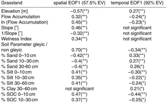
Table 1.Pearson correlation coefficients between EOFs and topographic and soil parameters

for the grassland test site; Curvature H/V, % Clay 0–10 cm, 10–30 cm and % SOC 30–60 cm were additionally tested but not significant; EV is the variance explained by the EOF.

Grassland spatial EOF1 (57.5% EV) temporal EOF1 (92% EV)

Elevation [m] −0.57(**) 0.27(**)

Flow Accumulation 0.32(**) −0.24(*)

ln (Flow Accumulation) 0.45(**) −0.23(*)

Slope [◦_] _0.46(**) _{not significant}

1/Slope [◦_]

−0.32(**) not significant

Wetness Index 0.34(**) not significant

Soil Parameter gleyic /

non gleyic 0.70(**) ₋0.34(**)

% Sand 0–10 cm ₋0.42(**) 0.33(**)

% Sand 10–30 cm ₋0.4(**) 0.27(**)

% Sand 30-60 cm ₋0.4(**) 0.26(*)

% Silt 0–10 cm 0.41(**) ₋0.30(**)

% Silt 10–30 cm 0.35(**) ₋0.22(*)

% Silt 30–60 cm 0.41(**) ₋0.24(*)

% Clay 30–60 cm not significant 0.21(*)

% SOC 0–10 cm 0.47(**) −0.44(**)

% SOC 10–30 cm 0.37(**) −0.25(*)

(27)

HESSD

6, 5565–5601, 2009

patterns

W. Korres et al.

Title Page

Tables Figures

◭ ◮

Back Close

Full Screen / Esc

Table 2.Pearson correlation coe_fficients between EOFs and topographic and soil parameters

for the arable land test site; EV is the variance explained by the EOF.

Arable land spatial spatial temporal

EOF1 (38.4% EV) EOF2 (28.2% EV) EOF1 (72% EV)

Elevation [m] ₋0.73(**) not significant 0.47(**) Surface Stone Cover [%] ₋0.79(**) not significant 0.48(**) Field Capacity [%] 0.75(**) not significant ₋0.41(**)

(28)

HESSD

6, 5565–5601, 2009

patterns

W. Korres et al.

Title Page

Tables Figures

◭ ◮

Back Close

Full Screen / Esc

Table 3.Pearson correlation coefficients between ECs and the soil moisture average from each

measuring campaign.

Soil Moisture Average [%]

Grassland spatial EC1 0.73(**) Grassland temporal EC1 ₋1.00(**)

Arable land spatial EC1 ₋0.71(**) Arable land spatial EC2 not significant Arable land temporal EC1 1.00(**)

(29)

HESSD

6, 5565–5601, 2009

patterns

W. Korres et al.

Title Page Abstract Introduction Conclusions References Tables Figures ◭ ◮ ◭ ◮ Back Close

Full Screen / Esc

Printer-friendly Version Interactive Discussion 1₀ 3 1 0 8 10₉ 1 1 0 1₀ 6 1₀ 4 1 0 2 10 1

Field borders 1 m contour lines

(height a. s. l.)

5 m contour lines

(height a. s. l.)

1 0 3 5 0 5 515 510 515 50 5 500 495 490 48 5 480 47 5 51 0 50˚37'25''N Measuring points F1 F2 F3 F4 F5 F6 F7 F8 F9 F5 F6 F4 F2 F1 F3 Field number F8 1 0₅ 1 0 7

Grassland Arable Land

50˚52'10''N

0 150 300

Meters

6˚18'16''E 6˚27'04''E

0 150 300

Meters

Fig. 1. Topography, field layout and measuring grid of the grassland (Rollesbroich) and the

(30)

HESSD

6, 5565–5601, 2009

patterns

W. Korres et al.

Full Screen / Esc

Printer-friendly Version Interactive Discussion 18 May 2007 19 June 2007 22 June 2007 28 August 2007 02 October 2007 05 October 2007 02 April 2008 29 April 2008 27 May 2008 03 June 2008 06 June 2008 28 August 2008 16 September 2008 19 September 2008 0 10 20 30 40 50 60 70 80 Surface Soil Moisture [Vol.-%] 41 ₄₂ 96 54 52 72 82 96 96 96 96 96 96 96

Fig. 2.Box-Whisker-Plot for the grassland site of all days of surface soil moisture measurement;

(31)

HESSD

6, 5565–5601, 2009

patterns

W. Korres et al.

Full Screen / Esc

Printer-friendly Version Interactive Discussion 15 May 2007 18 May 2007 19 June 2007 24 June 2007 27 July 2007 28 August 2007 02 October 2007 05 October 2007 29 April 2008 03 June 2008 06 June 2008 08 July 2008 25 July 2008 28 July 2008 28 August 2008 16 September 2008 19 September 2008 0 10 20 30 40 50 Surface Soil Moisture [Vol.-%]

44 59 104

56 118 118 118 90 118 118 118 100 ₁₁₈ 110 118 118 118

Fig. 3. Box-Whisker-Plot for the arable land test site of all dates of measurement; the bottom

(32)

HESSD

6, 5565–5601, 2009

patterns

W. Korres et al.

Title Page

Tables Figures

◭ ◮

Back Close

Full Screen / Esc

1 2 3 4 5 6 7 8

0 10 20 30 40 50 60 70 80

EOF Number

Explained

Variance

[%]

(a)

1 2 3 4 5 6 7 8

0 10 20 30 40 50 60 70 80 90 100 110 120 130 140

EOF Number

Explained

Variance

[%]

(b)

Fig. 4.Variance spectrum of the spatial(a)and temporal(b)analysis in the grassland test site.

(33)

HESSD

6, 5565–5601, 2009

patterns

W. Korres et al.

Title Page

Tables Figures

◭ ◮

Back Close

Full Screen / Esc

EOF Values

-0.2 - -0.1 -0.1 - 0.0 0.0 - 0.1 0.1 - 0.2 0.2 - 0.3 0.3 - 0.4 (a)

22

June

2007

29

April

2008

27

May

2008

03

June

2008

06

June

2008

28

August

2008

16

September

2008

19

September

2008

0 10 20 30 40 50 60

EC

value

0 10 20 30 40 50 60

Average

Soil

M

oisture

[Vol.-%]

(b)

Fig. 5. EOF1 (a)and EC1 (b) patterns of the spatial analysis in the grassland test site; the

(34)

HESSD

6, 5565–5601, 2009

patterns

W. Korres et al.

Title Page

Tables Figures

◭ ◮

Back Close

Full Screen / Esc

1 2 3 4 5 6 7 8 9 10

0 10 20 30 40 50

EOF Number

Explained

Variance

[%]

(a)

1 2 3 4 5 6 7 8 9 10

0 10 20 30 40 50 60 70 80 90 100 110

EOF Number

Explained

Variance

[%]

(b)

Fig. 6.Variance spectrum of the spatial(a)and temporal(b)analysis in the arable land test site.

(35)

HESSD

6, 5565–5601, 2009

patterns

W. Korres et al.

Full Screen / Esc

Printer-friendly Version Interactive Discussion 27 July 2007 28 August 2007 02 October 2007 29 April 2008 03 June 2008 06 June 2008 25 July 2008 28 August 2008 16 September 2008 19 September 2008 -40 -30 -20 -10 0 10 20 30 40 50 EC value 0 10 20 30 40 50 Average Soil Moisture [Vol.-%] (d) 27 July 2007 28 August 2007 02 October 2007 29 April 2008 03 June 2008 06 June 2008 25 July 2008 28 August 2008 16 September 2008 19 September 2008 0 10 20 30 40 50 EC value 0 10 20 30 40 50 Average Soil Moisture [Vol.-%] (c) EOF Values

-0.30 - -0.20 -0.20 - -0.10 -0.10 - 0.00 0.00 - 0.10 0.10 - 0.20

(a)

EOF Values

-0.20 - -0.10 -0.10 - 0.00 0.00 - 0.10 0.10 - 0.20 0.20 - 0.30

(b)

Fig. 7. EOF1(a), EOF2(b), EC1(c)and EC2(d)patterns of the spatial analysis in the arable

(36)