UNCERTAINTIES IN THE PREDICTION OF SPATIAL
VARIABILITY OF SOIL CO
2EMISSIONS AND RELATED
PROPERTIES
(1)Daniel De Bortoli Teixeira(2), Elton da Silva Bicalho(3), Alan Rodrigo Panosso(4), Luciano
Ito Perillo(3), Juliano Luciani Iamaguti(5), Gener Tadeu Pereira(6) & Newton La Scala Jr(6)
SUMMARY
The soil CO2 emission has high spatial variability because it depends strongly on soil properties. The purpose of this study was to (i) characterize the spatial variability of soil respiration and related properties, (ii) evaluate the accuracy of results of the ordinary kriging method and sequential Gaussian simulation, and (iii) evaluate the uncertainty in predicting the spatial variability of soil CO2 emission and other properties using sequential Gaussian simulations. The study was conducted in a sugarcane area, using a regular sampling grid with 141 points, where soil CO2 emission, soil temperature, air-filled pore space, soil organic matter and soil bulk density were evaluated. All variables showed spatial dependence structure. The soil CO2 emission was positively correlated with organic matter (r = 0.25, p < 0.05) and air-filled pore space (r = 0.27, p < 0.01) and negatively with soil bulk density (r = -0.41, p < 0.01). However, when the estimated spatial values were considered, the air-filled pore space was the variable mainly responsible for the spatial characteristics of soil respiration, with a correlation of 0.26 (p < 0.01). For all variables, individual simulations represented the cumulative distribution functions and variograms better than ordinary kriging and E-type estimates. The greatest uncertainties in predicting soil CO2 emission were associated with areas with the highest estimated values, which produced estimates from 0.18 to 1.85 t CO2 ha-1, according to the different scenarios considered. The knowledge of the uncertainties generated by the different scenarios can be used in inventories
(1) Part of the first author's dissertation. Received for publication in December 5, 2011 and approved in July 10, 2012.
(2) Post-Graduate Student, Agronomy Post-Graduate Program (Soil Sciences), UNESP/Jaboticabal. Via de acesso Prof. Paulo
Donato Castellani, s/n. CEP 14870-900 Jaboticabal (SP). E-mail: [email protected]
(3) Post-Graduate Student, Agronomy Post-Graduate Program (Vegetal Production), UNESP/Jaboticabal. E-mail:
[email protected], [email protected]
(4) Post-Graduate Student from the Agronomy UNESP/Jaboticabal. E-mail: [email protected] (5) Graduate Student, Agronomy, UNESP/Jaboticabal. E-mail: [email protected]
of greenhouse gases, to provide conservative estimates of the potential emission of these gases.
Index terms: soil respiration, geostatistics, ordinary kriging, sequential Gaussian simulation, sugarcane.
RESUMO: INCERTEZAS NA PREDIÇÃO DA VARIABILIDADE ESPACIAL DA EMISSÃO DE CO2 DO SOLO E PROPRIEDADES RELACIONADAS
A emissão de CO2 do solo apresenta alta variabilidade espacial, devido à grande dependência
espacial observada nas propriedades do solo que a influenciam. Neste estudo, objetivou-se: caracterizar e relacionar a variabilidade espacial da respiração do solo e propriedades relacionadas; avaliar a acurácia dos resultados fornecidos pelo método da krigagem ordinária e simulação sequencial gaussiana; e avaliar a incerteza na predição da variabilidade espacial da emissão de CO2 do solo e demais propriedades utilizando a simulação sequencial gaussiana. O estudo foi
conduzido em uma malha amostral irregular com 141 pontos, instalada sobre a cultura de cana-de-açúcar. Nesses pontos foram avaliados a emissão de CO2 do solo, a temperatura do solo, a
porosidade livre de água, o teor de matéria orgânica e a densidade do solo. Todas as variáveis apresentaram estrutura de dependência espacial. A emissão de CO2 do solo mostrou correlações
positivas com a matéria orgânica (r = 0,25, p < 0,05) e a porosidade livre de água (r = 0,27, p <0,01) e negativa com a densidade do solo (r = -0,41, p < 0,01). No entanto, quando os valores estimados espacialmente (N=8833) são considerados, a porosidade livre de água passa a ser a principal variável responsável pelas características espaciais da respiração do solo, apresentando correlação de 0,26 (p < 0,01). As simulações individuais propiciaram, para todas as variáveis analisadas, melhor reprodução das funções de distribuição acumuladas e dos variogramas, em comparação à krigagem e estimativa E-type. As maiores incertezas na predição da emissão de CO2 estiveram
associadas às regiões da área estudada com maiores valores observados e estimados, produzindo estimativas, ao longo do período estudado, de 0,18 a 1,85 t CO2 ha-1, dependendo dos diferentes
cenários simulados. O conhecimento das incertezas gerado por meio dos diferentes cenários de estimativa pode ser incluído em inventários de gases do efeito estufa, resultando em estimativas mais conservadoras do potencial de emissão desses gases.
Termos de indexação: respiração do solo, geoestatística, krigagem ordinária, simulação sequencial gaussiana, cana crua.
INTRODUCTION
In 2005, agriculture accounted for emissions of 5.1 6.1 Gt CO2-eq, representing 10-12 % of the global
emissions and making it the second largest source of anthropogenic emissions of greenhouse gases (GHGs) (IPCC, 2007). However, due to the complexity and uncertainty involved in quantifying soil carbon (C) balance, in most studies, estimates of GHG emissions from agricultural soils are included in those related to forestry and land use changes (IPCC, 2007). This complexity is due to the high spatial variability (La Scala et al., 2000; Panosso et al., 2009; Brito et al., 2010; Teixeira et al., 2011a,b) and temporal variability (Herbst et al., 2010; Teixeira et al., 2011a,b) in soil CO2 emissions (FCO2).
Spatial variations in FCO2 are primarily the result
of physical, chemical and biological soil properties such as organic matter content (Søe & Buchmann, 2005), carbon stock (Panosso et al., 2011), cation exchange capacity (La Scala et al., 2000 ), microbial biomass (Søe & Buchmann, 2005) and soil mineralogy (La Scala et al., 2000).
Geostatistical analysis has been used to describe the spatial variability of FCO2, using techniques such
several recent studies (Herbst et al., 2010, Teixeira et al., 2011a,b), providing an alternative to the smoothed values estimated by OK.
Because of the importance of sugarcane cultivation in the State of São Paulo and because of the uncertainty in the process of CO2 emission and
sequestration from agricultural soils, it is crucial to characterize the primary factors driving FCO2. This
study aimed (i) to characterize the variability and spatial distribution of FCO2 as well as physical and
chemical properties, such as air-filled pore space, soil temperature, organic matter content and bulk density (BD); (ii) to evaluate the accuracy of the results of OK and SGS; and (iii) to determine the uncertainty in predicting the spatial variability of the variables using SGS.
MATERIAL AND METHODS
The study was conducted on the Fazenda Santa Olga (21° 21' S, 48° 11' W), which belongs to the São Martinho Mill, in Guariba, São Paulo State. According to the Thornthwaite classification, the local climate can be defined as B1rB’4a’ - type mesothermal humid, with little water stress, evapotranspiration and less than 48 % annual evapotranspiration in the summer. The soil of the area was classified as high clay Oxisol (Eutrustox, USDA Soil Taxonomy).
Sugarcane (Saccharum spp. var. SP86-155), in a management system with mechanical harvesting, had been grown for eight years on the area. At the time of the study, the soil was devoid of vegetation and covered with large amounts of crop residue (12 t ha-1). On
July 13, 2010, a regular grid of 60 × 60 m was installed with 141 points, between 0.5 to 10 m away from the installation site of PVC rings, used to assess soil CO2
emissions (La Scala et al., 2000) (Figure 1).
The FCO2 was assessed using three portable systems (LI-COR 8100). The soil chambers were coupled to a system that quantifies the internal concentration of CO2 through optical absorption spectroscopy in the infrared spectral region. Before starting the experiment, the machines were tested and calibrated. The evaluations were conducted in the morning (8:00-9:30 h a.m.) over seven days, on Julian days 195, 196, 197, 200, 201, 204 and 207 in 2010 (Teixeira et al., 2011b). Concurrently with the assessment of FCO2 values, soil temperature was
measured with a sensor coupled to the analysis system (LI-8100) and moisture (% volume) was measured with a TDR (Time Domain Reflectometer) - Hydrosense system, both in the 0-0.10 m layer. After the evaluations, soil was sampled from the same layers by the volumetric ring method to obtain soil BD and total pore volume (TPV) (Embrapa, 1997). The air-filled pore space (AFPS) was obtained by the difference between the TVP and soil moisture. Disturbed
samples were also taken from the same sites to determine soil organic matter, using methods described by Raij et al. (1987). In the analysis, FCO2, temperature and AFPS were the average values of the seven days of evaluation.
Descriptive statistics (mean ± standard error, standard deviation, coefficient of variation, minimum, maximum, skewness and kurtosis) were previously used in the description of the variables to provide interpretations of geostatistical analysis. The spatial variability of the variables was determined using experimental variogram modeling based on the theory of regionalized variables, which is estimated by:
, ) ( ) ( ) ( 2
1 ) (
ˆ 2
) (
1
h x z x z h N
h i
h N
i
i - +
=
å
=
g [ [ (1)
where
γ
ˆ(h) is the experimental semivariance for a separation distance h, z(xi) is the property value atpoint i, and N(h) is the number of pairs of points separated by distance h. The variogram describes the spatial continuity of the variables as a function of the distance between two locations. In this study, spherical, exponential and Gaussian models were used.
The best fit to the variogram model used in the OK method was based on the cross validation, external validation, and the coefficient of determination (R2)
obtained for the model fit. For the variogram used in the simulation process, only the model’s coefficient of determination was considered, as it is a stochastic method and validations are available only after completing all stages of the process.
For external validation, 14 randomly selected points (10 % of the original data) (Teixeira et al., 2011a) were removed from the sampling grid (Figure 1) before creating the variogram model. The values observed at those points are then compared with the values estimated by OK and simulated by SGS at those points. In two validations (cross and external), observed and estimated values were used to calculate the root mean square error (RMSE).
( ) ˆ( ) ,
1 20,5
1 ïþ ï ý ü ïî ï í ì
-å
= n i ii z x
x z n
RMSE =
[
[
(2)where n is the number of values used in the validation, z(xi) is the property value at point i, and zˆ( )xi is the
estimated value of the property at point i. Smaller RMSE values indicate higher accuracy in the estimates.
Ordinary kriging is a weighted average of the neighboring samples, and the weights for each neighbor are determined through structural correlations in the data, represented by the semivariance gˆ(h) as a function of h (Equation 1) and
resulting in an estimate of minimum variance. The KB2D routine of the GSLIB - Geostatistical Software Library (Deutsch & Journel, 1998) was used to calculate OK estimates.
Stochastic simulations that reproduce the distribution reference points (data) are prioritized in relation to an optimal prediction with minimum variance estimation (OK). Several simulation algorithms are available. In this study, we used a SGS. In SGS, equiprobable maps of the distribution of variables are produced using the standard model of the variogram. The differences between the various outputs provide a measure of uncertainty in the prediction of spatial data. The stages of the SGS can be studied in more detail in Deutsch & Journel (1998).
In this paper, 300 realizations of each variable were considered. We randomly selected the 30th, 68th, 176th
and 214th realization of each variable to represent 300
individual simulations. We chose random realization to maintain the characteristics of the method, as the selection of outputs based on a specific parameter can limit the amount of uncertainty provided by the method. The SGS procedure was based on the SGSIM routine in the Geostatistical Software Library (Deutsch & Journel, 1998).
Maps of minimum, medium (E-type), maximum and standard deviation were produced by counting the simulated points at each location in the 300 realizations. Pearson’s analyses were conducted in the E-type estimates to compare the spatial patterns of the variables.
The accuracy and goodness-of-fit (G statistics) of the probability density function provided by the different interpolation methods were evaluated based
on the G statistics, as proposed by several authors (Goovaerts, 2001; Herbst et al., 2010; Bourennane et al., 2010). The simulated/estimated values and the original data located at intervals of probability p, defined by the limits (1-p)/2 and (1+p)/2, were compared using Fˆ(u,z(n)). Based on the cumulative density function (cdf) calculated for any location u of
) ) ( , ( ˆ u z n
F and z(uj) with j = 1, ... N, the fraction of
true values falling into a series of symmetrical probability intervals p is obtained by the equation:
[0,1] ) , ( 1 1 )
( =
å
" Î= p p u N N j j p x
x
,
(3)where x(uj,p) is given by:
î í
ì - < £ +
= -otherwise p u F u z p u F if p
u j j j
j 0 ) 2 / ) 1 ( , ( ˆ ) ( ) 2 / ) 1 ( , ( ˆ 1 ) , ( 1 1
x
(4)
Thus, to evaluate the proximity between simulated/ estimated fractions and the data set, we calculated the G statistic as shown below:
[ ]
ò
-
-= 1
0 3 ( )2 ( )
1 a p p pdp
G x
,
(5)where a(p):
î í ì ³ = otherwise p p if p a 0 ) ( 1 )
( x (6)
For inaccurate cases in which x(p)<p, the values of a(p) are twice as accurate as for cases in which
>p p) (
x . The best reproduction of the cdf is represented by a G value closer to 1.
According to Goovaerts (2001), the accuracy in the reproduction of the variogram can be evaluated by the following equation:
[ ] [ ]
å
= -= S s s s s h h h 1 2 2 ) ( ) ( ˆ ) ( g g geg , (7)
where S is the number of lags used to construct the variogram, and g(hs) is the semivariance in distance hs calculated from the estimated/simulated values.
Values close to 0 indicate good accuracy in the reproduction of the variogram.
To assess the quality of E-type estimates for each variable, the generated maps were subjected to external validation (Bourennane et al., 2010) based on the root mean square error (RMSE) (Equation 2) and mean error (ME) (Teixeira et al., 2011a) data by the following equations:
( ) ( )
[ ˆ ],
1 1
å
= -= n i ii z x
x z n
ME (8)
where n is the number of values used in the validation (n=14), z(xi) is the property value at point i, zˆ( )xi is
The ME and RMSE values provide, respectively, measures of bias and accuracy in the estimates generated, however due to the existence of different scales between variables, a comparison of these characteristics between them becomes inappropriate. This problem was solved by standardization of the indices using the standard deviations of each variable (Table 1) (Hengl, 2007).
RESULTS AND DISCUSSION
The average soil CO2 emission (1.57 ± 0.07 μmol m-2 s-1) in the evaluation period was lower than
reported in other studies in Oxisols for sugarcane areas (Panosso et al., 2011), a difference that may be related to a lack of rainfall in the days before the experiment; high soil compaction, as indicated by mean values of BD of 1.50 ± 0.01 g cm-3; and low
organic matter content (4.75 ± 0.05 g dm-3) (Table
1). Brito et al. (2009) evaluated soil respiration associated with sugarcane in a green harvest management system at different topographic positions and found average emission values from 2.39 to 2.97 μmol m-2 s-1. High variability in
emissions, characterized by a high CV value (50.02 %), has been reported in several studies, obviating the need for spatial characterization of this property using geostatistics (Teixeira et al., 2011a). The homogeneity observed in the soil temperature (CV = 1.69 %) is most likely related to the soil being covered with crop residues, which is characteristic of green management (Panosso et al., 2009).
The emission was positively linearly correlated with AFPS (r = 0.27, p < 0.01) and organic matter content (r = 0.25, p < 0.05) and negatively correlated with BD (r = -0.41, p < 0.01). The AFPS and BD directly impact the process of gas transport in soil, affecting both the entrance of oxygen, which is necessary for aerobic microbial activity, and the output of CO2, which is a byproduct of microbial activity.
The OM, in turn, is the primary source of energy used by the microbes, thus explaining its positive relationship with soil respiration.
Panosso et al. (2011) used multiple regression analysis to model the FCO2 in sugarcane areas under
green and slash-and-burn management, and they observed that the AFPS was selected for both models, being responsible for 18 % of the variability of FCO2
under sugarcane cultivation. Linn & Doran (1984) studied the effect of water-filled pores on soil respiration and found the highest rates of emission under conditions close to 60 % filling of the pores, at a density of 1.40 g cm-3, conditions very different from those
obtained in our study, in which, on average, only 37 % of the pores were filled with water.
Ohashi & Gyokusen (2007) studied the spatial and temporal variability of soil respiration in forest areas
(Cryptomeria japonica D. Don) and identified soil compaction as a factor related to emission. Although the present study did not find a correlation between emissions and soil temperature, the temperature can directly influence the production process by affecting the dynamics of soil microorganisms. The lack of correlation between temperature and respiration can be attributed to the low variability in temperature during the evaluations (Table 1).
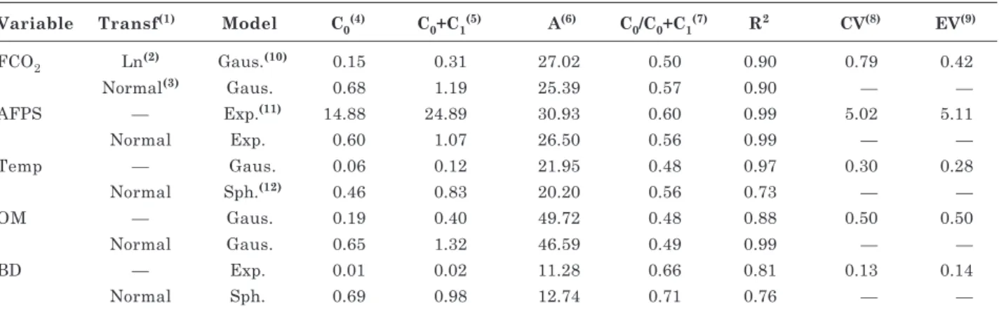
The structure of spatial variability was characterized by adjusting the variogram models (Table 2). For most geostatistical techniques, such as OK, a normal data distribution is not required; however, normality is desired to allow the inference of statistics such as maximum likelihood (Deutsch & Journel, 1998). Thus, a logarithmic transformation was used for FCO2 to correct the asymmetric values shown in Table 1. This procedure is often used to describe spatial FCO2 (Panosso et al., 2009; Herbst et
al., 2010; Teixeira et al., 2011b). After the FCO2
transformation, the normality of distribution was confirmed by the Kolmogorov-Smirnov test (p> 0.15). However, for predictions based on SGS, transformation should be performed to ensure the normality of the data (Table 2). After the spatial estimates are produced, in both cases, the estimated values are re-transformed to the original data scale again.
With the exception of temperature and BD, the same models were obtained for the unprocessed and processed data. For FCO2, Gaussian models were the
best fit, although in most other studies, spherical models (Brito et al., 2010; Herbst et al., 2010; Teixeira et al., 2011a) and exponential models (Panosso et al., 2009) fit better. Each model describes variability in different ways, and, along with the parameters, is responsible for the spatial patterns of each variable. The spherical model is appropriate for abrupt changes in variables with large distances, and the exponential model describes relatively irregular phenomena, whereas the Gaussian model is adopted for regular and continuous phenomena. Thus, the fit of the Gaussian model to the experimental variogram of FCO2 demonstrates that, despite the high variability
(Table 1), spatial distribution is smoothly distributed in space. This pattern could be due to the arrangement of points in the sampling grid used in this experiment and to the fact that the soil was covered by crop residues. The extremely dense sampling grid enabled the evaluation of small-scale variables (0.50 m), allowing the identification of similarity over short distances.
The degree of spatial dependence was classified as moderate for all variables, characterized by the relation 0.25 < C0/C0+C1 < 0.75 (Cambardella et al.,
et al. (2009) in their evaluation of the spatial uncertainty of soil water content.
Brito et al. (2010) and Panosso et al. (2009) studied the FCO2 in soils under sugarcane with green harvest management and found moderate spatial dependence structures. Herbst et al. (2010), evaluating the FCO2 in soil without vegetation,
found dependence structures ranging from weak to strong. The range obtained for FCO2 (27.02 m) was
similar to that found by Brito et al. (2010) for back-slope and foot-back-slope topographic positions for the the same soil type and vegetation. Panosso et al. (2009), using a sampling grid with 60 points spaced 13.30 m apart (190 × 50 m), observed values ranging from complete independence between the samples to near 73.2 m.
The correlation of FCO2 with the BD was closer
(r = -0.41, p < 0.01), but the high similarity between the ranges in the variogram models fitted to FCO2 (27.02 and 25.39 m) and AFPS (30.93 and 26.50 m) suggests a higher spatial correlation between them, which was possibly the variable with the strongest
influence on FCO2 in this study. The BD and OM had
lower (11.28 and 12.74 m) and higher (49.72 and 46.59 m) range values, respectively, indicating a lower spatial continuity in the BD around OM.
Each realization represents a realistic image of the spatial distribution of the variable without the smoothing effect created by OK (Delbari et al., 2009). The differences between the realizations provide alternative visual measures of the spatial uncertainty associated with estimates (Deutsch & Journel, 1998). The standard deviation maps represent the point variation in all simulated realizations (n=300); in other words, they represent the local uncertainty associated with predictions based on observed values and the sampling grid (Grunwald et al., 2007). Thus, the deviations become zero at the points of observed values, due to the conditional characteristic of the simulation (Figure 2). There is a predominance of high FCO2
values (> 3.30 μmol m-2 s-1), in the upper right and
center of the map, whereas low values (> 1.80 μmol m-2 s-1), are distributed throughout the area, but with
greater consistency in the upper portion of the map. Variable Mean SE(6) SD(7) CV(8) Min(9) Max(10) Skew(11) Kurt(12) KS(13)
FCO2(1) 1.57 0.07 0.79 50.02 0.34 4.08 0.86 0.14 < 0.01
AFPS(2) 34.21 0.44 5.22 15.26 22.95 49.15 0.14 -0.01 0.13
Temp(3) 19.40 0.03 0.33 1.69 18.50 20.33 -0.44 0.59 0.05
OM(4) 4.75 0.05 0.57 11.89 3.00 6.10 0.10 0.02 > 0.15
BD(5) 1.50 0.01 0.14 9.50 1.06 1.86 -0.25 0.39 > 0.15
Table 1. Descriptive statistics of soil CO2 emission and influential properties
n=141; (1) Soil CO
2 emission (μmol m-2 s-1); (2) Air-filled pore space (%); (3) Soil temperature (ºC); (4) Organic matter content (g dm-3); (5) Bulk density (g cm-3); (6) Standard error of the mean; (7) Standard deviation; (8) Coefficient of variation; (9) Minimum; (10)
Maximum; (11) Skewness; (12) Kurtosis; (13) p-value of Kolmogorov-Smirnov normality test.
Variable Transf(1) Model C
0(4) C0+C1(5) A(6) C0/C0+C1(7) R2 CV(8) EV(9)
FCO2 Ln(2) Gaus.(10) 0.15 0.31 27.02 0.50 0.90 0.79 0.42
Normal(3) Gaus. 0.68 1.19 25.39 0.57 0.90 — —
AFPS — Exp.(11) 14.88 24.89 30.93 0.60 0.99 5.02 5.11
Normal Exp. 0.60 1.07 26.50 0.56 0.99 — —
Temp — Gaus. 0.06 0.12 21.95 0.48 0.97 0.30 0.28
Normal Sph.(12) 0.46 0.83 20.20 0.56 0.73 — —
OM — Gaus. 0.19 0.40 49.72 0.48 0.88 0.50 0.50
Normal Gaus. 0.65 1.32 46.59 0.49 0.99 — —
BD — Exp. 0.01 0.02 11.28 0.66 0.81 0.13 0.14
Normal Sph. 0.69 0.98 12.74 0.71 0.76 — —
Table 2. Type of transformation used and parameters of models fitted to experimental variograms of soil CO2 emissions (FCO2), air-filled pore space (AFPS), soil temperature (Temp), organic matter content (OM) and soil bulk density (BD)
The standard deviation map associated with the estimation of FCO2 indicates that the deviation was greater for areas with high estimated values, which are more uncertain than the lowest values. This result is similar to that reported by Grunwald et al. (2007) for estimates of total soil phosphorus.
The various realizations randomly selected for the spatial representation of AFPS demonstrate some specific patterns, such as the presence of intermediate values, 32.95 to 40.45 %, in the upper right and center of the maps. For the soil temperature, consistently low values (< 16.75 °C) are observed in the upper left, whereas intermediate values (19.5 to 20.0 °C) are observed in the central portion of the images. The simulated values above 20.25 °C were associated with a large uncertainty throughout the entire area. Higher values of organic matter with high variability predominate in the central part of the map. Although areas with high BD values are evident in some realizations, their predictions are highly uncertain. For the soil temperature, the highest deviations were associated with lower predicted values. In contrast, for AFPS and BD, the greatest deviations were observed in regions with lower-density samples, as
similarly found by Delbari et al. (2009). For OM, high deviations are distributed across the entire experimental area.
The reproduction of the cumulative probability density functions (cdfs) and variograms of the interpolated data were used to evaluate the accuracy of the results provided by OK and SGS (Table 3). For all variables, the simulations better the individual cdfs and variograms reproduced when compared to OK, with values of G statistics and e(g) closer to 1 and 0, respectively. Again, the statistics displayed a high degree of similarity between the E-type estimates and those generated by OK (Table 3 and Figure 2). The low performance of OK in the reproduction of the variogram and cdfs shows that it should not be used when a reproduction of the statistics and variability structure of the data is desired.
Ergodic fluctuations, which are small differences between the observed values and those predicted by SGS, are produced at each step of the simulation procedure (Goovaerts, 2001) and play a key role in increasing uncertainty and making the estimate more conservative. The exact reproduction of these functions is only advisable when measuring the
accuracy and reliability of the samples (Deutsch & Journel, 1998).
Another factor that may influence the low reproduction of the cdfs and the variogram by the SGS, originates in the process of restructuring the variogram model due to normalization and the subsequent use of OK in the estimation of local averages, a procedure used to circumvent the lack of stationarity in the observed data (Deutsch & Journel, 1998). Bourennane et al. (2010) claim that all features of the simulation, including the use of simple or ordinary kriging, the maximum number of nodes simulated, the search radius and the choice of upper and lower values of interpolation, significantly affect the quality of the results.
According to Grunwald et al. (2007), the average represents the dominant property signal in the area, whereas the range of possible results is characterized by the minimum and maximum values, representing the best and the worst possible scenario for each variable. The FCO2 showed a mean variation in an
area from 0.36 to 3.85 μmol m-2 s-1, resulting in a
wide range of emission (from 0.18 to 1.85 t CO2 ha-1),
over a short time, in different scenarios. This wide range, although within the limits of observed values (Table 1), is due to the presence of areas with lower-density samples that resulted in extremely erratic estimates.
Considering the emissions for sugarcane cultivation reported by De Figueiredo & La Scala (2011) and the different estimates generated in this work, FCO2 is the primary source of emissions in
areas with green sugarcane management and is even higher than emissions from N fertilizers and
diesel, indicating a significant shift in the composition of greenhouse gas emissions. The map of the minimum FCO2 values shows significant homogeneity in the area, whereas that generated with the highest values is similar to the E-type estimate and the standard deviation map (Figure 2) shows lower values at the top and bottom left and center-right of the map.
The uncertainty associated with estimates of soil properties, combined with the construction of different scenarios, provides useful information on the possible patterns of soil respiration, a property that is extremely erratic and difficult to predict because many properties have a direct or indirect relationship with FCO2, with
very close interval values.
By the E-type estimates, spatial relationships could be established between FCO2 and other properties
(Figure 2). As indicated by the variogram (Table 2), the AFPS had the highest spatial correlation (r = 0.26, p < 0.01) with FCO2. Similarly to the AFPS, although less intense, the correlations of OM and soil temperature were also positive (0.13 and 0.04, respectively,p < 0.01). The BD had a correlation of -0.12 (p < 0.01). Although the soil temperature was correlated with FCO2 when spatial patterns were
considered, the spatial correlation for the other variables was lower, indicating the difficulty of predicting the spatial FCO2 based on factors that can influence it.
The external validation procedure is often used to compare the quality and application of different interpolation methods (Teixeira et al., 2011a,b); however, in this case, the performance of E-type estimates generated for each variable was evaluated (Bourennane et al., 2010) (Table 4). According to the MEs values, the estimates for the AFPS (-0.07) had the least bias among the variables, slightly underestimating the validation points. The FCO2 was
the variable with the greatest data underestimation, with a MEs value of -0.48. For soil temperature and BD, the models used in the simulation process overestimated the validation set.
OK(6) E-type SGS(7) 30 SGS 68 SGS 176 SGS 214
G statistics
FCO2(1) 0.26 0.25 0.28 0.28 0.53 0.48
AFPS(2) 0.38 0.27 0.29 0.66 0.64 0.69
Temp(3) 0.38 0.35 0.58 0.58 0.58 0.58
OM(4) 0.27 0.27 0.59 0.59 0.58 0.60
BD(5) 0.22 0.24 0.60 0.60 0.62 0.60
ε(γ)
FCO2 6.28 6.96 2.62 0.94 1.23 1.25
AFPS 5.61 8.38 0.30 0.18 0.20 1.22 Temp 6.16 6.54 0.16 0.32 0.13 0.25 OM 7.85 7.56 0.23 0.14 0.20 0.09 BD 8.80 7.95 0.18 0.30 0.19 0.28 Table 3. Evaluation of the goodness-of-fit (G statistics)
of the probability density function and accuracy in the reproduction of the variogram (εεεεε(γγγγγ))
(1) Soil CO
2 emission;
(2) Air-filled pore space; (3) Soil temperature; (4) Organic matter; (5) Soil bulk density; (6) Ordinary kriging; (7)
Sequential Gaussian simulation.
FCO2(1) AFPS(2) Temp(3) OM(4) BD(5)
ME -0.38 -0.34 0.05 -0.17 0.03
MEs -0.48 -0.07 0.15 -0.30 0.21
RMSE 0.90 5.32 0.28 0.52 0.14
RMSEs 1.14 1.02 0.85 0.91 1.02
Table 4. Mean error (ME), standardized mean error (MEs), root mean square error (RMSE), standardized root mean square error (RMSEs), applied to the external validation data for the E-type maps
n=14; (1) Soil CO
2 emission; (2) Air-filled pore space; (3) Soil
According to Hengl (2007), RMSEs values > 0.71 indicate that the models captured less than 50 % of the variability in the points used for validation. Although all RMSEs values were considered high, soil temperature was the variable with the most accurate estimates, with a value of 0.85. The soil temperature estimates were 7.06 (OM) to 34.12 % (FCO2) more
accurate than the other variables.
CONCLUSIONS
1. The strong relationships observed between the sampling points and spatial estimates of CO2
emissions (FCO2), bulk density and air-filled pore space suggest the utility of these as covariates in interpolation procedures of FCO2 to improve the accuracy of estimates of unsampled locations.
2. The configuration of the sampling grid and the soil covered with crop residues may have influenced the characterization of the spatial distribution of FCO2,
temperature and OM, leading to a more homogeneous distribution of these properties on a small scale (less than 3 m).
3. The individual simulations maintained the characteristics of the original data better than ordinary kriging, reproducing the original variograms and histograms.
4. By sequential Gaussian simulation, areas with higher uncertainties were identified for the estimated properties, which is particularly important for sample designs that reduce uncertainty and thus increase the spatial accuracy of the estimates.
LITERATURE CITED
BOURENNANE, H.; DOUAY, F.; STERCKEMAN, T.; VILLANNEAU, E.; CIESIELSKI, H.; KING, D. & BAIZE, D. Mapping of anthropogenic trace elements inputs in agricultural topsoil from Northern France using enrichment factors. Geoderma, 157:165-174, 2010. BRITO, L.F.; MARQUES, J.; PEREIRA, G.T. & LA SCALA, N.
Spatial variability of soil CO2 emission in different
topographic positions. Bragantia, 69:19-27, 2010. BRITO, L.F.; MARQUES, J.; PEREIRA, G.T. & SOUZA, Z.M.
Soil CO2 emission of sugarcane fields as affected by topography. Sci. Agric., 66:77-83, 2009.
CAMBARDELLA, C.A.; MOORMAN, T.B.; NOVAK, J.M.; PARKIN, T.B.; KARLEN, D.L.; TURCO, R.F. & KONOPKA, A.E. Field-scale variability of soil properties in central Iowa soils. Soil Sci. Soc. Am. J., 58:1501-1511, 1994.
DE FIGUEIREDO, E.B. & LA SCALA, N. Greenhouse gas balance due to the conversion of sugarcane areas from burned to green harvest in Brazil. Agric. Ecosyst. Environ., 141:77-85, 2011.
DELBARI, M.; AFRASIAB, P. & LOISKANDL, W. Using sequential Gaussian simulation to assess the ûeld-scale spatial uncertainty of soil water content. Catena, 79:163-169, 2009. DEUTSCH, C.V. & JOURNEL, A.G. GSLIB: Geostatistical Software Library and User’s Guide, 2.ed. New York, Oxford University Press, 1998. 369p.
EMPRESA BRASILEIRA De PESQUISA AGROPECUÁRIA -EMBRAPA. Centro Nacional de Pesquisa de Solos. Manual de métodos de análise de solo. 2.ed. Brasília, 1997. 212p.
GOOVAERTS, P. Geostatistical modeling of uncertainty in soil science. Geoderma, 103:3-26, 2001.
GRUNWALD, S.; REDDY, K.R.; PRENGER, J.P. & FISHER, M.M. Modeling of the spatial variability of biogeochemical soil properties in a freshwater ecosystem. Ecol. Model, 201:521-535, 2007.
HENGL, T.A. Practical guide to geostatistical mapping of environmental variables. Roma, AJRC Scientific and Technical Reports, 2007. 165p.
HERBST, M.; PROLINGHEUER, N.; GRAF, A.; HUISMAN, J.A.; WEIHERMÜLLER, L.; VANDERBORGHT, J. & VEREECKEN, H. Multivariate conditional stochastic simulation of soil heterotrophic respiration at plot scale. Geoderma, 160:74-82, 2010.
INTERGOVERNMENTAL PANEL ON CLIMATE CHANGE -IPCC. Climate change 2007: The physical science basis. Summary for policymakers. Geneva, Switzerland. Available at: <http://www.ipcc.ch/>. Accessed: Nov 3, 2011. LA SCALA, N.; MARQUES, J.; PEREIRA, G.T. & CORÁ, J.E. Short-term temporal changes in the spatial variability model of CO2 emissions from a Brazilian bare soil. Soil
Biol. Biochem. 32:1459-1462, 2000.
LINN, D.M. & DORAN, J.W. Effect of water-filled pore space on carbon dioxide and nitrous oxide production in tilled and non-tilled soils. Soil Sci. Soc. Am. J., 48:1267-1272, 1984. OHASHI, M. & GYOKUSEN, B. Temporal change in spatial
variability of soil respiration on a slope of Japanese cedar
(D. Don) forest. Soil Biol. Biochem., 39:1130-1138, 2007. PANOSSO, A.R.; MARQUES, J.; MILORI, D.M.B.P.; FERRAUDO, A.S.; BARBIERI, D.M.; PEREIRA, G.T. & LA SCALA, N. Soil CO2 emission and its relation to soil
properties in sugarcane areas under Slash-and-burn and Green harvest. Soil Tillage Res, 111:190-196, 2011. PANOSSO, A.R.; MARQUES, J.; PEREIRA, G.T. & LA SCALA,
N. Spatial and temporal variability of soil CO2 emission
in a sugarcane area under green and slash-and-burn managements. Soil Tillage Res., 105:275-282, 2009. RAIJ, B.van; QUAGGIO, J.A.; CANTARELLA, H.; FERREIRA,
M.E.; LOPES, A.S. & BATAGLIA, C.O. Análise química do solo para fins de fertilidade. Campinas, Fundação Cargill Campinas, 1987. 171p.
TEIXEIRA, D.D.B.; PANOSSO, A.R.; CERRI, C.E.P.; PEREIRA, G.T. & LA SCALA, N. Soil CO2 emission estimated by
different interpolation techniques. Plant Soil, 345:187-194, 2011a.
TEIXEIRA, D.D.B.; BICALHO, E.S.; PANOSSO, A.R.; PERILLO, L.I.; IAMAGUTI, J.L.; PEREIRA, G.T. & LA SCALA Jr., N. Krigagem ordinária e simulação sequencial Gaussiana na interpolação da emissão de CO2 do solo. R.