Condition-based maintenance considering shock and degradation processes

(1)

* Corresponding author.

Decision Science Letters 6 (2017) 151–164

Contents lists available at GrowingScience

Decision Science Letters

homepage: www.GrowingScience.com/dsl

Condition-based maintenance considering shock and degradation processes

Hossein Rahimi Komijania_{, Mahdi Shahin}b*_{, Mohammad bagher Shahin}c_{and Armin Jabbarzadeh}b

a_{Department of Industrial Engineering, K.N.Toosi University,Tehran, Iran}

b_{Department of Industrial Engineering, Science and Technology University,Tehran, Iran} c_{Department of Industrial Engineering, urmia University, Iran}

C H R O N I C L E A B S T R A C T

Article history: Received June 25, 2016 Received in revised format: October 22, 2016 Accepted October 22, 2016 Available online October 24 2016

An important issue in maintaining the industrial equipment is to introduce an appropriate maintenance policy to monitor the conditions of the equipment. In this research, an investigation on the concurrent effects of erosion and random shocks during the useful life of the equipment is studied. In this regard a model is introduced to optimize the total cost including logistic, complete repair and incomplete repair costs. The proposed model determines the optimal number of the incomplete repairs, the time duration between inspections and the probability of equipment to be failed. A numerical example is solved by means of computer simulation. The results indicate that the proposed model performs well for minimizing the costs of maintenance and repair.

Condition monitoring Erosion

Random shocks

Complete and incomplete repair

1. Introduction

(2)

the screening process of equipment. According to Bloch and Geitner (1983), the main incentive for the application of condition-based maintenance is based on the assumption that approximately 99 percent of equipment failures are caused by specific symptoms, conditions, or warnings appeared before failures happen. However, according to Jardine et al. (2006), the life span of equipment is determined through the review and screening of operational conditions, and these conditions occur through several parameters that are known as condition monitoring parameters. Some of these parameters include vibration, temperature, noise or any other contamination. Maintenance models are provided based on several categories (for further information see Cui et al., 2010).

The article is organized as follows: At first we present a literature review and show some gaps in the literature. After that we will describe equipment, and model assumptions and parameters. Then, equations are provided to define the distribution function for the random shocks due to the remaining life span. Then, we introduce the model and present a numerical example to evaluate its performance. Finally, the results will be discussed.

2. Literature Review

Zhang (2007) used the geometric process to introduce repairable equipment that is in decline with three phases and the optimal policy was obtained through minimizing the average cost. In practice, many systems are exposed to different and separate types of shocks and these shocks may be classified based on size, function, and effect types. Some studies have addressed the reliability of multi-component systems where the system is influenced by the independent risks of burnout and a set of random shocks. In Song et al. (2014), in contrast to previous studies in which only a simple system was affected by the same shock, random shocks fall into several categories based on the size and performance. The shocks may only be effective on one or more components of complex systems (instead of all of its components) based on specific classification. Yu et al. (2014) studied the systems affected by random shocks and the shocks trend to reach the system was the phase type. In this system, it is assumed that the maximum shock tolerance of the system is reduced by the increased number of repairs. Also, time intervals between repairs increased after every repair and the system is replaced upon reaching a certain amount of repairs.

In Montoro-Cazorla and Pérez-Ocón (2014), system reliability when subjected to shock damage was studied in which some shocks causing damage and the others causing a failure in the system, as well as this failure can be repairable or non- repairable. Repair times are calculated based on phase type distributions and the model calculates availability, reliability and failure rate of different failure types. Other similar studies carried out in the simultaneous presence of shock and erosion variable in which the shock to the system is derived from environmental conditions of equipment. According Zhu et al. (2015), for example, the decline of the system was obtained from the sum of burnout and shock damage, and burnout was calculated on the basis of non-static gamma process and cumulative shock based on generalized Pareto distribution. Wang et al. (2011) proposed a developed method based on Wiener process to estimate the remaining and thus decisions based on the conditions, where drift coefficient were linear in every part of the process but non-linear in the whole process, unlike the conventional method. This advantage of this method is the impact of past data efficiency in estimation. This method is comparative and the comparison implementation is based on Kalman filter.

(3)

H. Rahimi Komijani et al. / Decision Science Letters 6 (2017)

including replacement and incomplete (e.g., minor repair) both run, and appropriate maintenance policy is determined on the basis of status variables. Tian et al. (2011) proposed multi-objective models in the optimization condition-based maintenance, with regard to both maximize reliability and minimize cost. They used physical planning approach in the optimization problem. Xiang et al. (2012) proposed a method to approximate this distribution as most distributions functions had high-complexity until the time of failure and studied a single equipment unit. In this equipment the rate of moment failure depends on the stage in which the equipment is located and the desired point is introduced in Markov space.

Wang (2012) reviewed the existing literature and proposed a delay time-based maintenance model. The model is one of mathematical methods for optimization and determines inspection time. In this method equipment failure is divided into two stages: the first stage starts from the time the equipment starts work until the time of a failure occurs, the second stage starts from the assumed point of time until equipment failure moment. Such a model has a completely random nature. Simultaneous cumulative effect of shock and erosion variables in equipment are used to determine the optimal maintenance policy. The amount of damage caused by shock or repeated function of these systems can be determined through some measurable physical characteristics. The equipment is not able to work at their satisfactory level when monitoring indicators reach a certain level, and then it must be replaced or repaired. In condition based maintenance it is possible to make decision based on the current situation of the equipment in determining the appropriate time to complete repair, incomplete repair and or inspection. The equipment condition in incomplete repair is something between its original state (such as a new equipment) and the condition before the failures (Brown & Proschan, 1983). Literature speaks of many incomplete maintenance policies, in the first policy, the efficient life of equipment with incomplete repair is reduced. This approach has many applications in optimization models because of its simplicity. The second policy considers improvements factor where any incomplete maintenance operations causes changes in failure rates and reliability of equipment. The third policy studies possible approaches by which incomplete maintenance with probability P puts the equipment to the initial state and with probability 1-P leaves is to the same state. Other policies relate to the degradation and erosion of the equipment that could be affected by a variety of random shocks models. In this approach, the effect of maintenance operations is shown as reducing the degree of damage or the damage level.

Literature review indicates that none of the current research is to investigate the presence of shock and erosion variables in addition to all possible states of repair (complete maintenance, incomplete maintenance, and corrective maintenance) a long with a variety of logistics costs imposed on the system (lost opportunity costs) and the possibility of failures. Most maintenance policies are only based on a combination of several factors above. The aim of this study is to provide a comprehensive maintenance policy that is able to obtain the optimal amount of the cost function for maintenance operations given the presence of shock and erosion variables as well as the cost and time of logistics. Also, introduced a probability distribution function to determine the secondary shock variable after any incomplete maintenance is among other innovations in this paper. The structure of logistics costs and times is determined according to reference (Do Van et al., 2013).

3. System Description, Assumptions and Parameters

(4)

of an incomplete repair, and therefore shock and erosion variables secondary status, is determined by probability distribution function. Shock and erosion variables are assumed to be independent which are valid in a lot of sophisticated equipment. Most gas turbines experiencing burnout in constant operation over times, but other factors such as thermal shocks can affect the equipment function independent of burnout due to the turbine structure complexity. Engine valves may be damaged as a result of burnouts over time or failure caused by burns (thermal shocks) or mechanical shocks. Evidently, many new valves are at risk of failure because of the existence of such shocks (mechanical and thermal). Therefore, burnout and sudden failure resulting from shock can be considered independent because of the nature and minimal dependence between them. Industrial engines may break due to the mechanical shocks in operation time in addition to fatigue caused by work.

The destructive shocks into the equipment can be caused by human errors in the deployment of equipment; for example, these errors accumulate over time in equipment that are frequently set up and used, therefore, these errors are independent of burnout. Human errors include such as incorrect setup process or installation errors in the shaft that leads to the bent shaft. Naturally, shock and fatigue damage is independent in human errors. Also, both variables may be considered independent when the equipment burnout values at any moment have low ratio given the amount of damage caused by any shock. In some studies, shock and burnout variables dependent assumption are on the grounds that shocks inflicted in the system as a result of equipment the external setting (operating conditions) and equipment burnout in terms of the internal conditions of the system (Shafiee et al., 2015).

The variables used in the model are as follows:

: Random variable of cumulative damage caused by the shock to the time t

: Random variable of amount of burnout caused by the operation of equipment (Weiner variable) to the time t

: Random variable of time remaining until the equipment failure after the i-th inspection for erosion variable

: Random variable of time remaining until the equipment failure after the i-th inspection for cumulative shock variable

: Random variable of the amount of damage to the equipment at the time of j-th shock : Random variable of number of shocks to equipment to the time t

: Random variable of shock level after the last incomplete repair at the time

. : Probability density distribution function of remaining lifetime of equipment on the basis of variable erosion

. : System state probability density distribution function after the implementation of each incomplete repair

: : Erosion variable values vector to i-th inspection , , … , : Shock variable First Passage Time (FTP) over the threshold

W: Equipment failure threshold due to shock random variable

: The risk of damage or equipment failure given the inspection time intervals and the number of incomplete operations

: The number of incomplete maintenance operations

: Time of running a complete maintenance for when erosion variables are passing failure threshold : Time of running an incomplete maintenance for when erosion variables are passing failure threshold : Time of running a complete maintenance (replacement) or a corrective maintenance operation

( ، )

: Costs rate per unit time (loss of productivity) to perform preventive maintenance (complete or incomplete repair)

: Costs rate per unit time (loss of productivity and expenses related to the system burnout) to perform corrective maintenance

: The cost per unit for inspection

(5)

: Incomplete maintenance cost of damaging shock variable

: Fixed costs of preparing and logistics for each incomplete maintenance for shock variable : Fixed costs of preparing and logistics for each incomplete maintenance for erosion variable : Complete maintenance operations cost

: Corrective maintenance operations cost

: Incomplete maintenance cost to complete maintenance cost ratio for the value of improvement in

the erosion process (

: Incomplete maintenance cost to complete maintenance cost ratio for the value of improvement in

the shock process (

Τ : Preparation time for corrective maintenance or replacement.

Τ : Preparation time for incomplete maintenance with relation to damaging shock

Τ : Preparation time for incomplete maintenance with relation to burnout

3.1 Cumulative Damage Caused by Shock

Variable t , i.e., variable of cumulative damage caused by the shock to the time t, that is

Z t y ,

(1)

where, y is the damage inflicted on equipment in the time of j-th shock and N t is the number of shocks to equipment to time t.

Figure 1 shows the event structures and the amount of damages.

Fig. 1. Shock structures and the amount of damages.

The basic assumptions of shock models as included by Shafiee et al. (2015) are valid here.

The equipment is under shocks that the distribution of shocks event follows non-homogeneous Poisson process, .

Any shocks causes damages in the equipment that the amount of the damages in all the shocks follow the same distribution, the shocks are independent of each other, as well as the distribution of the number of shocks at the time of ( ) is independent of random variable of the amount of damage, ( ). The amount of damage caused by shocks is added to the current level of damage.

The current level of damage ( ), increases only if shock occur.

(6)

interval , ] is shown as . Average number of shocks in this interval is equal to . The probability that the shock jth ( ) is before time , is shown with and is equal to:

, (2)

.

The probability distribution of the amount of damage inflicted by a shock is given by

and the amount of damage caused by the j-th shock is the same as . Thus, according to the second assumption and are independent of each other as well as the number of shocks in time (i.e., random variable . The total amount of damage caused by a number of j shock is calculated as follows:

∑ , ≡ , (3)

where, is the amount of damage caused by the occurrence of j-th shock that has happened to the current time. According to (Cox, 1962), the distribution of variable is calculated via Convolution

, as follows:

(4)

,

The total amount of damage ( ) to time t, depends on the number of shocks that occurs in the interval

, .

(5)

According to the second assumption and using the theory of probability and independence between

, , … and , we can write:

,

Since ∑ and , probability distribution total damage can be written as:

Replacing and in the equation , in the last equation, the

total damage probability distribution function is simplified as:

(6)

Damage changing behavior due to random shocks is given in Figure 2. Equipment failure threshold for the cumulative shock variable is shown by W. The first passing time of shock variable from failure limit shown by equals to:

: (7)

(7)

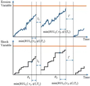
is the amount of damage caused by shocks to remains on equipment after the -th incomplete maintenance operation. In other words, is the value of the damage caused by shock after incomplete repair that is zero for ; i.e., ( .

Fig. 2. The process of increasing damage due to shock inflicted on the equipment to reach the failure limit

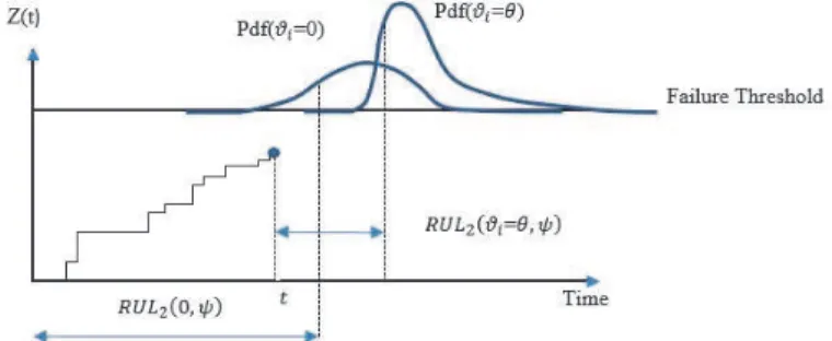
The remaining life is considered as the remaining life of the equipment in which the possibility of equipment failure does not exceed a certain amount. As a result, the remaining life of the equipment failure that the possibility of equipment failure ( ) does not exceed a certain amount:

, : , (8)

where, is the remaining time to reach the failure limit in i-th inspection (at the time ). Fig. 3 shows the process of updating the distribution function of the remaining time to failure for shock process. In the first start-up time ( ), the system remaining lifetime based on shock variable has probability density distribution of ( ), thus estimated remaining life time of a given probability of failure ( ) is equal to , that is area under the probability density function graph in Figure 3. Then, after observing the state of shock at the time , and the corresponding probability density functions , estimated remaining lifetime, assuming the probability of failure ( ) in this case is equal to the area under the chart .

Fig. 3. The process of updating the remaining life distribution of the shock damage

3.2 Cumulative Damage Caused by Erosion

(8)

, (9)

where, is initial amount of damage, and are drift and diffusion parameters, respectively. is also standard Brown motion that show dynamic random part of the damage process. The remaining life time with a given probability of failure is defined as:

, : | : | : ,

(10)

where, is the remaining time variable to i-th equipment failure after the inspection. _: is erosion variable values vector to i-th inspection period. The cost of any incomplete maintenance for shock damage variable is determined as follows:

,

∗ (11)

where, is the cost of preparation and logistics in each incomplete maintenance operation, is the cost of lack of production at the time of incomplete maintenance operation given the shock. Other costs in the original model are similar to the structure presented in (Do Van et al., 2013).

4. The proposed model

The ultimate goal of the maintenance policy is to determine the appropriate time period (time interval between inspection operations, ∆ ), the number of incomplete maintenance operation ( ) and the probability of failure ( ). Three types of possible operations are intended to equipment in the proposed model, including corrective maintenance, complete preventive maintenance and incomplete preventive maintenance. Corrective maintenance is applied in case of equipment failure and preventive maintenance is applied before the failure occurs, corrective maintenance and complete preventive maintenance operations returned equipment to the initial state but incomplete preventive maintenance puts the equipment in intermediate state. Preparation time and logistics (including procurement and order the necessary parts, etc.) for both preventive operations is similar and equal toΤ . Improved process for the shock variable after any incomplete maintenance is obtained using Truncated Gamma distribution, which is defined as follows:

f x|a, b x Z _{F Z} _{b Γ a x} e

a E N t γ k, η

b _γ_∗ Z_{k, η} (12)

γ k, η k η b

γ∗ _{k, η} _b _k _η _b

(9)

of shocks on the average situation after the repair increases when is closer to 1. value has a direct impact on the effectiveness of cost ratio on probability distribution function. The reason behind the use of Truncated Gamma distribution is the strong character of this distribution given changing its parameters to produce variety of other probability distributions.

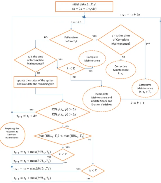
Fig. 4. Maintenance decision-making process

The cost ratios are involved in determining the status of system recovery after running an incomplete maintenance comes from the idea that the higher incomplete maintenance costs and closer to the complete maintenance costs more improvements in the system can be expected. For example, by replacing several major components of the system (which is costly), one can imagine that equipment gains very favorable condition than to replace only one of its sub-components (with incomplete maintenance cost less). The values initial estimate for determining the parameters of Truncated Gamma distribution is according to the experts (Gaoini et al., 2009). Then, equipment secondary status data was used for the estimation. Maintenance policy decision algorithm is graphically presented in Fig. 4. To be precise in each discrete time , , …) the appropriate decisions are made according to the conditions: if the equipment fails before inspection time , immediately all necessary resources (spare parts, maintenance tools, maintenance operators, etc.) are ordered to perform corrective maintenance. If the equipment is still in working condition to time , an inspection operation is done and the current

Initial data∆ , ,

)

, , =_∆

(

Fail system

before ?

Corrective Maintenance in Corrective Maintenance in Incomplete

Maintenance and update Shock and Erosion Variables Complete Maintenance

update the status of the system and calculate the remaining life

is the time of Complete Maintenance?

is the time of Incomplete Maintenance? yes yes yes yes yes no yes yes no no no no no yes no no

Preparing the resources to

carry out maintenance

max ,

max , max ,

∆

, ∆

(10)

state of equipment (shock damage and erosion level) is obtained. Finally, based on the recent data obtained the introduced methods are used to calculate remaining time to the failure (i.e., , and , values). A description of the maintenance policy listed to the situation that the incomplete maintenance optimum number 1( is as Fig. 5. The total cost function according to Do Van et al., (2013) that is modified by taking the cost of shock into account is defined as follows,

∆ , , , (13)

where, is the number of damages and is the number of complete maintenance operations or the replacement and and are the number of incomplete operations related to each variable of the status and is the number of inspections to time . is the total number of incomplete operations on both variables of the status. is the length of time that the equipment is in pause mode due to failure.

Fig. 5. The optimal policy for maintenance operations when K = 1

The long-term expected cost rate method is a conventional optimization method in determining the maintenance functions. The long-term expected cost rate is defined based on renewal theory as follows.

∆ , , → ∆ , ,

(14)

The purpose of this type of maintenance policy is to appropriately determine optimal inspection time interval for maintenance (∆ ), the total number of incomplete maintenance ( ) and the possibility of equipment failure at inspection time interval ( ). The optimum level of decision parameters obtained from the following equation

∆ ∗_, ∗_, ∗

∆ , , ∆ , , , ∆ ∞, (15)

Simulation is used to evaluate different scenarios to find the optimal values of the parameters given the complexity of the Eq. (15). The simulation is done in a long time, thus the optimal parameter for decisions on maintenance policy is determined taking the average of a large number of the results of the simulation.

5. Numerical examples

(11)

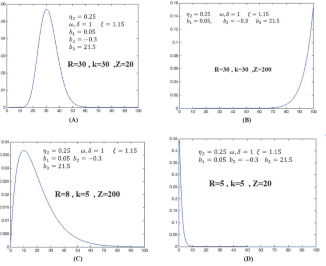
Fig. 6. different modes (A, B, C, D) with various amounts of shock and incomplete maintenance and cumulative shock level

Probability density functions of several variables to determine the secondary shock is produced by changing the mean number of shocks and the level of damage caused by the shock , and the number of incomplete maintenance operations, ( ) that is the total number of incomplete maintenance operations for both status. Fig. 6 considers the value equal to R for the sake of simplicity. Accordingly, it is evident that increased each of these variables results in probability density function of distribution skewed to the right turns to skewed to the left. This means that equipment status leads to more adverse conditions after implementation of incomplete preventive maintenance for increasing the number of incomplete maintenance operations as well as the final status of implementation of the number of imposed shocks. Fig. 7 shows various probability distributions can be produced based on two different values for the incomplete maintenance costs to replacement costs ratio. Variable parameters in various forms to include various cost ratios. Two modes are drawn for . 5 and . . The numerical example parameters values for Weiner process and random shocks is intended as follows:

5

5 5

(12)

Fig. 7. various probability distributions for the erosion variable given the elapsed lifetime and the number of incomplete maintenance operations (A and B)

Erosion variable secondary status is determined by Do Van et al. (2013) and according to Fig. 7-A with assumption . 5. The probability density function for the secondary status after incomplete repair of damage caused by shock is determined according to Fig. 6 with assumption . 5. The number of shocks over time process follows Poisson distribution with √ parameter. The optimal values for ∗ . %, ∗ , and ∆ ∗ obtained through simulation calculations. This means that the optimum inspection time is implemented at ∆ ∗ intervals, and the optimal number of incomplete maintenance equals to ∗ units and the probability of failure equals to ∗ . %. The values of cost rate function ( ∆ , , ) given the number of incomplete maintenance for sensitivity analysis based on simulated data are shown in Table 1.

Table 1

Values of expected cost rates according to the changes in the number of incomplete maintenance operations

K ∆ , , ∆τ Ψ [%] K ∆ , , ∆τ Ψ [%]

0 68 53 0.3 8 30.7 44 0.41

1 50 48 0.03 9 3932 1.18

2 43 39 1.5 10 35 51 0.38

3 37 27 1.11 11 4238 0.05

4 35 31 0.67 12 41 39 1.6

5 33 36 0.66 13 2744 0.49

6 31 25 1.6 14 48 35 0.93

7 30.1 33 0.13

Also, the results of Table 2 were obtained via sensitivity analysis on the costs ratio values. The results of Table 2 show the effects of cost ratios on determining the optimal number of incomplete maintenance. Thus, the fixed and variable costs values for incomplete maintenance are provided to obtain equal ratios of and .

Table 2

Sensitivity analysis based on 1 and 2 values

1

η η2 ∆τ K* Ψ*[%] CoR (∆τ,K*, Ψ*)

0.25 0.25 33 7 0.13 30.1

0.3

0.3 48 0.46 33.7

0.4 0.4 43 6 0.5 40.2

0.5

0.5 39 0.84 47.5

0.7 0.7 45 1 1.1 59.12

0.95

(13)

Fig. 8. Values of expected cost rates according to the changes in the number of incomplete maintenance operations

6. Conclusion and Recommendation

The current paper represented the appropriate condition based maintenance policy for equipment with operational state which was determined by two variables of shock and erosion. Three types of maintenance operations were considered including complete preventive maintenance, incomplete preventive maintenance, and corrective maintenance. Truncated Gamma distribution for the shock variable in determining the possible incomplete repair of equipment after every repair was introduced. Here, four different modes were studied given the level of destructive shock ( ), the number of incomplete maintenance function ( and the cost ratio ( ) were used to describe the shock variable. optimal values for three decision variables, i.e., inspection intervals, the number of incomplete maintenance operations and the possibility of equipment failure calculated by simulations. The simulation results for the shock variable showed the more number of incomplete operations and the final level of shock value and the less its cost ratio , probability density function of distribution skewed to the right turns to skewed to the left. Optimal probability of failure and equipment failure ( ) and optimal inspection time intervals (∆ ) values have not fixed process due to the non-linear nature of cost function. The results showed that the optimal number of incomplete repairs reduces with increasing cost ratios, 1 and 2; such an outcome is not unexpected because the increased cost of incomplete repairs and approaching to the cost of replacement, it is logical to run replacement maintenance instead of incomplete maintenance. Models which assume dependency of shock and erosion variables can be recommended in future research. Also, detailed study of burnout effects based on the type of shocks to the equipment can be subject of a further work, as well. Given the uncertain status of the alert level, proposing a model with probability space of the erosion and shock warning can be examined as a future research topic.

References

Bloch, H. P., & Geitner, F. K. (1983). Practical machinery management for process plants. Volume 2:

Machinery failure analysis and troubleshooting (RPRT). Exxon Chemical Co., Baytown, TX.

Brown, M., & Proschan, F. (1983). Imperfect repair. Journal of Applied Probability, 851–859. JOUR. Cox, D. R. (1962). Renewal theory (Vol. 58). BOOK, Methuen.

(14)

Do Van, P., Voisin, A., Levrat, E., & Iung, B. (2013). Remaining useful life based maintenance decision making for deteriorating systems with both perfect and imperfect maintenance actions. In

Prognostics and Health Management (PHM), 2013 IEEE Conference on (pp. 1–9). CONF, IEEE.

Gaoini, E., Dey, D., & Ruggeri, F. (2009). Bayesian modeling of flash floods using generalized extreme

value distribution with prior elicitation. BOOK, University of Connecticut, Department of Statistics.

Jardine, A. K. S., Lin, D., & Banjevic, D. (2006). A review on machinery diagnostics and prognostics implementing condition-based maintenance. Mechanical Systems and Signal Processing, 20(7), 1483–1510. JOUR.

Last, M., Sinaiski, A., & Subramania, H. S. (2011). Condition-based Maintenance with Multi-Target Classification Models. New Generation Computing, 29(3), 245–260. JOUR.

Montoro-Cazorla, D., & Pérez-Ocón, R. (2014). A reliability system under different types of shock governed by a Markovian arrival process and maintenance policy K. European Journal of

Operational Research, 235(3), 636–642. JOUR.

Peng, Y., Dong, M., & Zuo, M. J. (2010). Current status of machine prognostics in condition-based maintenance: a review. The International Journal of Advanced Manufacturing Technology, 50(1– 4), 297–313. JOUR.

Shafiee, M., Finkelstein, M., & Bérenguer, C. (2015). An opportunistic condition-based maintenance policy for offshore wind turbine blades subjected to degradation and environmental shocks.

Reliability Engineering & System Safety, 142, 463–471. JOUR.

Si, X.-S., Wang, W., Hu, C.-H., & Zhou, D.-H. (2011). Remaining useful life estimation–A review on the statistical data driven approaches. European Journal of Operational Research, 213(1), 1–14. JOUR.

Song, S., Coit, D. W., & Feng, Q. (2014). Reliability for systems of degrading components with distinct component shock sets. Reliability Engineering & System Safety, 132, 115–124. JOUR.

Tian, Z., Jin, T., Wu, B., & Ding, F. (2011). Condition based maintenance optimization for wind power generation systems under continuous monitoring. Renewable Energy, 36(5), 1502–1509. JOUR. Tian, Z., Lin, D., & Wu, B. (2012). Condition based maintenance optimization considering multiple

objectives. Journal of Intelligent Manufacturing, 23(2), 333–340. JOUR.

Wang, W. (2012). A simulation-based multivariate Bayesian control chart for real time condition-based maintenance of complex systems. European Journal of Operational Research, 218(3), 726–734. JOUR.

Wang, W., Carr, M., Xu, W., & Kobbacy, K. (2011). A model for residual life prediction based on Brownian motion with an adaptive drift. Microelectronics Reliability, 51(2), 285–293. JOUR. Xiang, Y., Cassady, C. R., & Pohl, E. A. (2012). Optimal maintenance policies for systems subject to

a Markovian operating environment. Computers & Industrial Engineering, 62(1), 190–197. JOUR. Yu, M., Tang, Y., Wu, W., & Zhou, J. (2014). Optimal order-replacement policy for a phase-type

geometric process model with extreme shocks. Applied Mathematical Modelling, 38(17), 4323– 4332. JOUR.

Zhang, Y. L. (2007). A discussion on “A bivariate optimal replacement policy for a repairable system.”

European Journal of Operational Research, 179(1), 275–276. JOUR.

Zhu, W., Fouladirad, M., & Bérenguer, C. (2015). Condition-based maintenance policies for a combined wear and shock deterioration model with covariates. Computers & Industrial

Engineering, 85, 268–283. JOUR.