Development of New Algorithm for Voltage Sag Source Location

(1)

Abstract— Voltage sag is among the major power quality disturbances that can cause substantial loss of product and also can attribute to malfunctions, instabilities and shorter lifetime of the load. Accurate voltage sag source location can help to minimize the loss and problems caused by voltage sag in a power distribution system. This paper presents a development of a current component index (CCI) algorithm to locate the source of voltage sag in a power distribution system. The product of the RMS current and the power factor angle at the monitoring point is employed for the sag source location. A graph of this product against time is plotted. The voltage sag source location is determined by examining the magnitude of the current component index at the beginning of the sag. If the magnitude of the CCI during sag is higher than the magnitude of CCI before sag, it indicates that the voltage sag source is in front of the monitoring point. On the other hand if the magnitude of the CCI during sag is lower than the magnitude of CCI before sag, it indicates that the voltage sag source is in behind the monitoring point. The proposed method has been verified by simulations on a radial distribution system. Comparative studies with other method namely, the slope of the line fitting parameters of current and voltage method were also conducted in order to highlight the strength of the proposed method

Index Terms— Voltage sag, Single source, current.

I. INTRODUCTION

oltage sag is a temporary decrease in the RMS voltage magnitude between 0.1 – 0.9 p.u and with duration of mostly less than 1 second. Its frequency of occurrence is between a few tens and several hundreds times per year [1]. It is the most important power quality problem facing many industrial customers since equipment used in modern industrial plants such as process controllers and adjustable speed drives is becoming more sensitive to voltage sag. The causes of voltage sags are fault conditions, motor starting, transformer energizing and other sudden load changes. Voltage sags are typically caused by fault conditions [2], in which short-circuit faults and earth faults are found to cause severe voltage sags [3]. In industrial and commercial power systems, faults on one-feeder tend to cause voltage drops on all other feeders in the plant [4]. During short circuit faults, voltage sags occur whenever fault current flows through fault impedance. Voltage returns to normal as soon as a

Manuscript received October 31, 2008. N. Hamzah is with the Universiti Teknologi MARA, 40450 Shah Alam, MALAYSIA. (phone: 603-5543 5030; fax: 603-5543 5077; e-mail: noralizah@salam.uitm.edu.my ). A.Mohamed, is with Universiti Kebangsaan Malaysia, 47600 Bangi, MALAYSIA. (e-mail: azah@vlsi.eng.ukm.my). A. Hussain is with Universiti Kebangsaan Malaysia, 47600 Bangi, MALAYSIA. (e-mail: aini@vlsi.eng.ukm.my).

fault-clearing device interrupts the flow of current. These faults may be far from the interrupted process, but close enough to cause problems throughout the system. Even when voltage returns to normal, many sensitive loads experience a production outage if the voltage sag magnitude and duration are outside the load ride-through capabilities.

Locating the source of voltage sag is important before any voltage sag mitigation technique is done to eliminate the sag. A wrong mitigation solution can aggravate the voltage sag problem because only after information about a voltage sag source location is available, can power-quality trouble-shooting, diagnosis and mitigation be carried out. The advantage of locating the source of voltage sag is that any disputes among the major responsibility party can be resolved fairly [5].

To date only four references cite the methods to locate the sources of voltage sags from the literature. A method using the disturbance power and disturbance energy to determine which side of a recording device the voltage sag originates is based on the concept that active power tends to flow away from a nonlinear load [6]. This concept is translated in terms of disturbance power and disturbance energy to determine on which side of a recording device the voltage sags originate. The directions of the disturbance energy as well as the disturbance of real power flow are used to locate the voltage sag source. The method will rely on the degree of confidence of both the disturbance power and disturbance energy. Thus, the degree of confidence will be reduced if results from disturbance energy and disturbance power do not match. Another most recent technique to locate the origin of voltage sag is by employing the slope of the line fitting parameters of current and voltage during voltage sag [5]. The method plots the product of voltage magnitude and power factor against current magnitude at a particular measurement point. A line fitting of the measured points are performed and the sign of the slope indicates the direction of voltage sag source. A positive slope shows that the sag is from upstream and a negative slope shows that it is from downstream. The method has only been verified using three-phase-to-ground faults. Reference [7] applies the concept of instantaneous energy direction for voltage sag source detection which is claimed to be able to locate the voltage sag source. The other method is by applying the state estimation theory to estimate the location of voltage sag [8].

Faults in distribution system have been well known as a major cause of voltage sag. Hence this paper focuses on the development of new algorithm which is based on fault in a distribution power system. The proposed algorithm utilizes the phase angle difference between current and voltage or

Development of New Algorithm for Voltage Sag

Source Location

N. Hamzah, IEEE, A. Mohamed, Senior Member IEEE, A. Hussain, IEEE

(2)

power factor angle to determine the voltage sag source. In the method, magnitude of currents and phase angles of voltages and currents are measured at the monitoring point. The rms current is then multiplied with the cosine of the power factor angle and the product is then plotted against time. The product polarity is used to indicate the direction of voltage sag source either it is from behind the monitoring point or in front of the monitoring point. The proposed method is verified on a test distribution system modeled using an electromagnetic transient program EMTDC/PSCAD and the data are processed via MATLAB codes.

II. VOLTAGE SAG SOURCE LOCATION FOR SINGLE SOURCE SYSTEM ANALYSIS

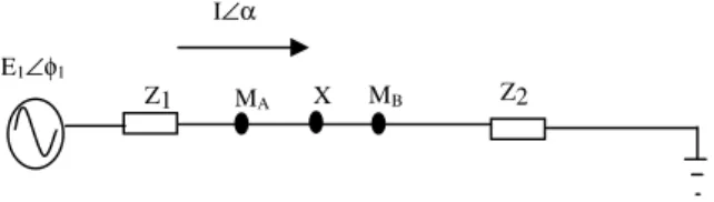
The index developed to determine the direction of the voltage sag source from the monitoring is based on the single source system in Fig. 1. In the figure, the direction of current is as shown.

From Fig. 1 the current flows before sag occurs is as seen from E1 and given by,

δ

φ

α

∠

=

∠

Z

E

I

1 1

(1) in which, Z∠δ is the line impedance and E1∠φ1 is the voltage

source. Before sag occurs, there is only one loop and the current that flows is I∠α. Assume there is fault at point X in which the impedance is given by Zf∠δ as in Fig. 2, two loops

are created. The voltage at point X will be very small or approaching zero [9], and the current namely as I1, I2 and If

will be created. Current I1 flows from source E1∠φ, I2 flows

from the fault point X and If flows through the fault

impedance to ground. From Fig. 2, the direction of I1 is

similar with the direction of current before fault occurs, I∠α

since it is from the same source, E1 and the current flows

towards X. If the impedance Z2 is higher than the fault

impedance Zf, current I2≈ 0 and the current from the source

E1 will flow towards Zf. Otherwise, the current I2 will flow

from Zf but the value is smaller than the value of current

before fault occurs. The current direction either it is from the source of voltage sag or towards the source of voltage sag will be used to develop the new indicator for determining the location of source of voltage sag.

A. Development of Current Component Index

The derivation of the proposed Current Component Index (CCI) to locate the source of voltage sag is based on the single line diagram as shown in Fig. 3(a). In the figure, assuming that the fault occurs at point X and the monitoring points are at MA

and MB. The direction of current before and after faults will

be considered. The positive direction of the current is from E1

to the monitoring X.

Before short circuit fault occurs at point X, and by applying the Kirchoff Current Law, the current at point MA or MB, is

given by,

α

θ

φ

α

−

∠

=

∠

T

Z

E

I

1 1

(2) In which,

θ : voltage angle at monitoring point

α: current angle at monitoring point

The phase difference (θ-α) is a power factor angle and

2 1 Z Z

ZT = + . From (2),

*

I

is given by,

T

T Z

E Z

E

I

φ

θ

α

θ

φ

α

= ∠− − +

− ∠

− ∠ = −

∠ 1 1 1 1 ₍₃₎

By multiplying the voltage at the monitoring point,

V

∠

θ

, with the left and right hand side of (3), the following equation is obtained,

T

Z

E

V

I

V

∠

θ

∠

−

α

=

∠

θ

1

∠

−

φ

1

−

θ

+

α

(4) By considering only the real power, equation (4) will provide the following,

T

Z

V

E

VI

cos(

_θ

_α

)

1

cos(

α

−

φ

1

)

=

−

(5) For a practical case, the angle (θ-α) are only between zero and 90o, i.e, the first quadrant of current lagging voltage case and

Fig. 2 Single source system during fault E1∠φ1 Z1∠δ1

I1

N

Z2∠δ2

I2 If

Zf∠δf X

Source 1 E1∠φ1

Z∠δ

I∠α

N

Fig. 1 Single source system before fault

Fig. 3 (a) Single source system for voltage sag analysis before faults occur

MA MB

E1∠φ1

X

Z1 Z2

(3)

in the third quadrant of current leading voltage case. In order to obtain the current value, both sides of equation (5) will be divided with V, hence the current component flowing from E1

will produce,

T

Z

E

I

cos(

_θ

₋

_α

)

₌

1

cos(

α

−

φ

1

)

₍₆₎

Thus from equation (6), the current before fault, Icos( - )bf

from E1 to the monitoring point X is given as,

T bf

Z

E

I

cos(

_θ

₋

_α

)

₌

1

cos(

α

−

φ

1

)

₍₇₎

Equation (7) is thus the current component index before fault occurs and can be written as CCIbs= Icos(θ-α)bf.

Fig. 3(b) shows the equivalent circuit when fault occurs at point X. By referring to MA as the monitoring point, the

source of fault is in front of the point MA. In the figure, Zf and

If, is the fault impedance and current respectively.

During fault, the voltage at X is very small, i.e, almost zero. Thus, current flows from E1 to the monitoring point X is

given by,

α

θ

φ

α

− ∠

∠ = ∠

1 1 1 Z

E

I (8) From equation (8),

I

* is given by,

1 1 1

Z E Z

E

I

φ

θ

α

θ

φ

α

= ∠− − +

− ∠

− ∠ = −

∠ (9)

The power equation can be obtained by multiplying both right and left hand side of equation (9) with the voltage at the monitoring point,

V

∠

θ

, as follows,

1 1 1

Z E V I

V∠

θ

∠−

α

= ∠

θ

∠−

φ

−

θ

+

α

(10) By considering the real power component, the following equation 11 can be given as follows,

1 1 1 cos( )

) cos(

Z V E

VI

θ

−

α

=

α

−

φ

(11)

To obtain the current values, the left and right hand side of equation (11) is divided with voltage, V, hence the current component that flows from E1 is given as follows,

1 1 1cos( )

) cos(

Z E

I

θ

−

α

=

α

−

φ

(12) Therefore, the current component during fault, i.e, Icos( - )f

from E1 to the monitoring point X, is given by,

1 1 1

cos(

)

cos(

Z

E

I

θ

−

α

_f

=

α

−

φ

(13) Equation (13) is the current component index during fault and can be written as CCIs = I cos(θ-α)f.

By dividing equation (13) with equation (7), we can obtain,

1 1

)

cos(

)

cos(

)

cos(

)

cos(

Z

E

Z

E

I

T

T bf

f

=

−

=

−

φ

α

φ

α

θ

α

θ

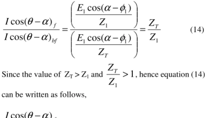
(14)

Since the value of ZT > Z1 and

1

>

Z

_T

, hence equation (14) can be written as follows,

1 )

cos(

)

cos(

>

−

bf f

I

α

θ

α

θ

(15) Equation Icos( - )bf and Icos( - )f is the current

component index before and during fault respectively. Therefore equation (15) re-written as,

bs

s

CCI

>

(16) Where CCIs and CCIbs is the current component index during

and before fault respectively.

From equation (16), it can be concluded that, at the beginning of voltage sag, if the current component index during fault is higher than current component index before fault, i.e, CCIs >

CCIbs, the source of voltage sag is in front of the monitoring

point, MA.

Next, it is to consider if the fault occurs at point X, which is behind the monitoring point MB, in which before fault occurs,

the current component index is similar as in equation (7). Fig. 4 shows the current when fault occurs at point X and the monitoring point is at point MB.

By referring to Fig. 3(a) and Fig. 4, during short circuit fault at point X, by applying Current Kirchoff Law, the current component at point MB is as follows,

Fig. 4 Voltage sag a equivalent circuit system for single source during fault and the monitoring point is at MB

MB E1∠φ

X

Z1 Z2

If∠θf Zf

I∠α

Fig. 3(b) Single source system for voltage sag analysis during fault and monitoring point at MA

MA E1∠φ1

V

∠

X

Z1 _Z

2

I

f

∠

Zf

(4)

)

cos(

)

cos(

)

cos(

_f

I

_bf

I

_f _f

I

θ

−

α

=

θ

−

α

−

θ

−

α

(17) In which, phrases Icos( - )f and Icos( - )bf is the current

during fault and current before fault at point MB respectively.

The phrase Icos( f- f) is the current equation which flows

through fault impedance, Zf, in which, f : voltage angle at fault location f : current angle at fault location.

From equation (17), it can be seen that the current during fault, which is Icos( - )f is less than the current component

before fault, Icos( - )bf.

Thus, by replacing the terms Icos( - )f and Icos( - )bf

with the terms CCIs and CCIbs, it can be seen that at

monitoring point MB, at the beginning of voltage sag, if CCIs

< CCIbs then, the location of the source of voltage sag is

behind the monitoring point.

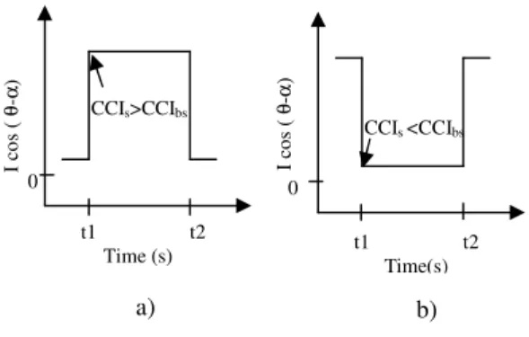
The proposed Current Component Index (CCI), i.e, Icos(θ-α), is the product of r.m.s current and power factor. This index is plotted against time as shown in Fig. 5. Fig. 5(a) shows the plot when the location of the voltage sag source is in front of the monitoring point. On the other hand, the plot when the source of voltage sag is behind the monitoring point is plotted in Fig. 5(b). In the figures t1 and t2 is the beginning

and end of the voltage sag duration respectively.

III. IMPLEMENTATION OF THE CURRENT COMPONENT INDEX

The proposed method to locate the source of voltage sags is verified on a test distribution system modeled using an electromagnetic transient program PSCAD/EMTDC. The procedure implemented is as follows:

(i) Detect the beginning of the voltage sag.

(ii) Obtain the magnitude and phase of voltage and current from the monitoring point at pre-fault and during fault times.

(iii)Calculate the values of Icos(θ-α) for a few cycles of pre-fault and during fault durations.

(iv)Graphically plot coordinates of Icos(θ-α) against time of a few cycles of pre-fault and during fault durations. Check the polarity of Icos( - )bf and Icos( - )f at the

beginning of fault. If CCIs < CCIbs then, the location of the

source of voltage sag is behind the monitoring point. On the other hand if CCIs > CCIbs, the source of voltage sag is in front

of the monitoring point.

IV. TEST SYSTEM AND RESULTS

The test system used in this study is as shown in Fig. 6. The system is fed by a voltage source of 33kV, 15MVA at 50 Hz frequency. By referring to Fig. 6, four fault locations have been considered, which are F1, F2, F3 and F4, whereas the monitoring points are PCC, M1, M2 and M3. Two types of faults have been simulated namely balanced and unbalanced faults. The three phase balanced faults have been simulated for about 0.3 seconds. On the other hand the unbalanced faults simulated are the single line fault (SLF) and double line fault (DLF).

A. Balanced Faults

Results of voltage sag which is caused by balanced faults are tabulated in Table I. By referring to Fig. 6, details of results from observation for the monitoring points and their respective fault location can be obtained. Table I presents the details of fault location and monitoring points simulated for the test system in Fig. 6.

TABLEI

DETAILS OF BALANCED FAULTS FOR A SINGLE SOURCE SYSTEM

Fault Location

Monitoring points

Sag source in front Sag source behind

F1 M1, PCC M2, M3

F2 M3, PCC M1, M2

F3 PCC M1, M2, M3

F4 M1, M2, M3 PCC

M2

3

Fig. 6 Test System For Voltage Sag 33 kV

33/11 kV, 15 MVA

F1 F3

F4 PCC

M3 M1

F2 1

2

4 5 9

6 7 8

1 1 19

1 13 14

15 16 17 18 2 0

Fig. 5 Index for Voltage Sag Source Location for Single Source System (a) In Front of Monitoring Point (b) Behind the Monitoring Point

I

co

s

(

θ

-α

)

a)

I

co

s

(

θ

-α

)

t1 t2

Time (s) CCIs>CCIbs

0

b) t1 t2

Time(s) CCIs <CCIbs

(5)

Fig. 7 shows the plots of CCI against currents for monitoring points at M1, M2 dan M3 for balanced faults at point F1. In Fig. 7a), it can be seen at the beginning of voltage sag, at t = 0.42 s, the value of CCI during sag is higher than the value of CCI before sag occurs, i.e, CCIs > CCIbs. This result

indicates that the source of voltage sag is in front of the monitoring point. The results for the monitoring at points M2 and M3 plotted in Fig. 7b) and c) show that at the beginning of voltage sag, the value of CCI during sag is lower than the values of CCI before sag, i.e, CCIs < CCIbs. Both results show

that the source of voltage sag is behind the monitoring points. These results prove that the CCI index can be used to locate the source of voltage sag and the results are in a good agreement with the observation in Table I.

B. Unbalanced Faults

In this paper, results from unbalanced fault are also presented for various points of monitoring points of Fig. 6. Two types of unbalanced faults are considered namely, single line to ground fault (SLF) and double line to ground faults (DLF). Table II presents the details of an unbalanced faults at F2 and the results obtained at monitoring points M1, M2, M3 and PCC. This information is then used to justify the accuracy of the simulation results using the CCI.

TABLEII

DETAILS OF UNBALANCED FAULTS FOR A SINGLE SOURCE SYSTEM

Fault Location F2 Monitoring Points Sag source

in front

Sag source behind Single Line to Ground

Fault (Phase A)

PCC, M3

M1, M2 Double Line to Ground

Faults, (Phase A)

PCC, M3

M1, M2 Double Line to Ground

Faults, (Phase B)

PCC, M3

M1, M2

The results of unbalanced faults (SLF) created at F2 are presented and analyzed. Fig.8 a), b) and c) show the graph of current component index against time for fault at F2 and the monitoring points at M1, M2 and M3 respectively. In Fig. 8a) and b), it can be seen that at the beginning of voltage sag, CCIs

< CCIbs. These results indicate that the source of voltage sag is

behind the monitoring points M1 and M2. On the other hand the result of the monitoring point at M3 shows that at the beginning of fault, CCIs > CCIbs (Fig. 8c). This result

indicates that the source of voltage sag is in front of the

monitoring point, M3. Thus, in the case of unbalanced fault, the CCI is able to accurately locate the source of voltage sag relative to its monitoring points as compared to the details in Table II.

The results of unbalanced faults (DLF) created at F2 are also presented and analyzed. Fig. 9 shows the result of CCI plotted against time obtained at monitoring points M1, M2 and M3. Fig. 9a) and 9b) show that at the beginning of faults the value of CCIs < CCIs, which indicate that the source of voltage sag

is behind the monitoring points. On the other hand, Fig. 9c) shows that CCIs > CCIbs indicating that the source of voltage

sag is in front of the monitoring point. From these results, the CCI therefore is accurate in indicating that the source of voltage sag is in front of the monitoring point as compared to the details in Table II.

C. Comparative Studies With Other Method

This section presents the comparison analysis between the CCI and Slope Of The Line Fitting Parameters Of Current and Voltage [5] method. Table III tabulates the comparison results for the balanced fault. The fault location is at F1 as shown in Fig. 6. The results in Table III are for monitoring points of PCC, M1, M2 and M3. From the table it can be seen that at monitoring points PCC and M1, both methods indicate the source of voltage sag is in front of the monitoring point. On the other hand, at monitoring points M2 and M3, both methods indicate that the source of voltage sag is behind the monitoring points.

Fig. 8 Results of CCI for unbalanced faults (SLF) at F2 for monitoring points, phase A, a) M1 b) M2 and c) M3. CCI s > CCI bs CCI s < CCI bs

I

co

s

(

θ

-α

)

(

k

A

)

Time (s) CCIs<CCIbs

Time (s) _{Time (s)}

I

co

s

(

θ

-α

)

(

k

A

)

I

c

o

s

(

θ

-α

)

(

k

A

)

I

co

s

(

θ

-α

)

(

k

A

)

CCI s > CCI bs

CCI s< CCI bs

I

co

s

(

θ

-α

)

(

k

A

)

CCI s < CCI bs

(c) Fig. 7 Balanced Faults at F1 for monitoring points a) M1 b) M2 and c) M3.

Time (s) Time (s) Time (s) (b)

(a)

I

co

s

(

θ

-α

)

(

k

A

)

Fig. 9 Results of CCI for unbalanced faults (DLF) at F2 for monitoring points, phase A, a) M1 b) M2 and c) M3.

I

co

s

(

θ

-α

)

(k

A

)

Time (s) CCI s < CCI bs

CCI s < CCI bs

Time (s)

I

co

s

(

θ

-α

)

(k

A

)

CCI s > CCI bs

Time (s)

I

co

s

(

θ

-α

)

(k

A

(6)

TABLEIII

COMPARISON OF VOLTAGE SAG SOURCE FOR BALANCED FAULTS FOR A SINGLE SOURCE SYSTEM, FAULT LOCATION AT F1 Monitoring

Points

Slope of the Line Fitting Parameters of Current and Voltage

Current

Component Index

PCC, M1 In Front of Voltage Sag Source

In Front of Voltage Sag Source

M2, M3 Behind of Voltage Sag Source

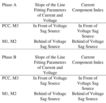
Behind of Voltage Sag Source Table IV tabulates the comparison results for the unbalanced fault (DLG) for a test system in Fig. 6. Results for phase A and Phase B for monitoring points PCC, M1, M2 and M3 are tabulated for comparison between Slope of the Line Fitting Parameters of Current and Voltage and CCI methods. From the table it can be seen that for phase A, at monitoring points PCC and M3, both methods indicate that the source of voltage sag is in front of the monitoring point. On the other hand, at monitoring points M1 and M2, both methods indicate that the source of voltage sag is behind the monitoring points. Similarly for phase B, both methods are in a good agreement in indicating that the source of voltage sag is in front and behind the monitoring points.

TABLEIV

COMPARISON OF VOLTAGE SAG SOURCE FOR UNBALANCED FAULTS (DLG) FOR A SINGLE SOURCE SYSTEM, FAULT LOCATION AT F2

Phase A Slope of the Line Fitting Parameters

of Current and Voltage

Current Component Index

In Front of Voltage Sag

Source M1, M2 Behind of Voltage

Sag Source

Behind of Voltage Sag Source Phase B Slope of the Line

Fitting Parameters of Current and

Voltage

Current Component Index

In Front of Voltage Sag

Source M1, M2 Behind of Voltage

Sag Source

Behind of Voltage Sag Source However, the implementation of the CCI is simpler than the Slope Of The Line Fitting Parameters Of Current and Voltage because the CCI only requires the voltage and current data. On the other hand the Slope Of The Line Fitting Parameters Of Current and Voltage method requires a line fitting technique on the top of current and voltage data to locate the source of voltage sag.

V. CONCLUSION

This paper has presented a new algorithm development to locate the source of voltage as seen at the monitoring points by examining the value of the current component index at the beginning of the voltage sag. From the results, it has been

proven that the CCI satisfy 100% of the voltage sag source location for balanced and unbalanced faults for the one source system. The advantage of the CCI can be listed as follows:

• It only requires three parameters for calculations, namely the magnitude for current and the phase angles of voltage and current at the monitoring points.

• It has been proven to work well with both balanced and unbalanced faults in a single source distribution system or radial system.

The method also can be used for a two-source system which will be published in our next paper.

VI. REFERENCES

[1] M. H. J. Bollen, “Voltage Sags in Three-Phase Systems”, IEEE Power Engineering Review, September 2001, pp.8-15, 17.

[2] M. H. J. Bollen, Understanding Power Quality Problems, IEEE Press, 2000, pp. 1-34.

[3] M. F. McGranaghan and D. R. Mueller, “Voltage Sags in Industrial systems”, IEEE Trans. On Industry Applications, Vol. 29, No. 2, March/April 1993, pp. 397-403.

[4] IEEE Std. 1159-1995: Recommended Practice for Monitoring Electric Power Quality, ISBN 1-55937-549-3.

[5] C. Li, T. Tayjasanant, W. Xu and X. Li, “ Method for voltage sag source detection by investigating slope of the system trajectory”, IEE Proc. Gener. Transm. Distrib., Vol. 150, No. 3, May 2003, pp. 367-372.

[6] A. C. Parsons, W. M. Grady, E. J. Powers and J. C. Soward, “A Direction Finder For Power Quality Disturbances Based Upon Disturbance Power and Energy”, IEEE Transactions On Power Delivery, Vol. 15, No. 3, July 2000, pp.1081-1086.

[7] W. Khong, X. Dong and Z. Chen, “Voltage Sag Source Location Based on Instantaneous Energy Detection, Proc. Of The 8th_{Int. Power} Engineering Conference 2007, 3-6 Dec 2007, pp. 90-94.

[8] H. Liao, “ Voltage sag Source Location in High-Voltage Power Transmission Networks”, Proc. IEEE Power and Energy Soceity General Meeting- Conversion and Delivery of Electrical Energy in the 21st_{Century, 20-24 July 2008, pp. 1-4.}

[9] McGranaghan, M. F, Mueler, D. R. & Samotyj,. Voltage Sags in Industrial Systems. IEEE Transaction Industry Application. M. J. 1993, 29 (2), pp. 397-403.

VII. BIOGRAPHIES

N. Hamzah received her B.Eng. (Hon) and M.Sc. (Power System), from University of Wales Institute of Science and Technology, UK in 1988 and University of Malaya, Malaysia in 1993 respectively. She obtained a PhD in Electrical Engineering (Power Quality) from the Universiti Kebangsaan Malaysia in 2006. She is an associate professor and head of program at the faculty of Electrical Engineering, University Teknologi MARA, Malaysia. She has published more than 50 technical papers in national and international conferences and journals. Her research interests include power quality studies, application of advanced signal processing in power system and artificial neural network studies. A. Mohamed received her B.Sc.Eng. from King’s College, University of London in 1978 and M.Sc. and PhD (Power System), from University of Malaya, Malaysia in 1988 and 1995, respectively. She is currently a professor at Universiti Kebangsaan Malaysia (UKM), Malaysia. Her current research interests are in power quality and other power system studies.