Journal of Multivariate Analysis

Contents lists available atScienceDirect

Journal of Multivariate Analysis

journal homepage:www.elsevier.com/locate/jmva

Optimal generalized truncated sequential Monte Carlo test

Ivair R. Silva

a,b,∗

, Renato M. Assunção

c,1

a_{Department of Statistics, Federal University of Ouro Preto, Belo Horizonte, Minas Gerais, Brazil}

b_{Department of Population Medicine, Harvard Medical School and Harvard Pilgrim Heath Care Institute, Boston, MA, United States} c_{Department of Statistics, Federal University of Minas Gerais, Belo Horizonte, Minas Gerais, 31270-901, Brazil}

a r t i c l e i n f o

Article history:

Received 2 August 2012 Available online 25 June 2013

AMS subject classifications:

62L05 62L15 65C05

Keywords:

Execution time Power loss

p-value density Resampling risk

a b s t r a c t

When it is not possible to obtain the analytical null distribution of a test statistic U, Monte Carlo hypothesis tests can be used to perform the test. Monte Carlo tests are commonly used in a wide variety of applications, including spatial statistics, and biostatistics. Conventional Monte Carlo tests require the simulation ofmindependent copies fromUunder the null hypothesis, what is computationally intensive for large data sets. Truncated sequential Monte Carlo designs can be performed to reduce computational effort in such situations. Different truncated sequential procedures have been proposed. They work under restrictive assumptions on the distribution ofUaiming to bound the power loss and to reduce execution time. Since the use of Monte Carlo tests are based on the situations where the null distribution ofUis unknown, their results are not valid for the general case of any test statistic. In this paper, we derive an optimal scheme for truncated sequential Monte Carlo hypothesis tests. This scheme minimizes the expected number of simulations under any alternative hypothesis, and bounds the power loss in arbitrarily small values. The first advantage from this scheme is that the results concerning the power and the expected time are valid for any test statistic. Also, we present practical examples of optimal procedures for which the expected number of simulations are reduced by 60% in comparison with some of the best procedures in the literature.

©2013 Elsevier Inc. All rights reserved.

1. Introduction

The Monte Carlo test (MC) is an important tool to perform hypotheses tests when the distribution of the test statistic

under the null hypothesis is unknown. Monte Carlo hypothesis testing is commonly applied in a wide variety of subject

areas. The Scan statistic, [9], directed to detect spatial cluster is an example of a Monte Carlo test application in spatial

statistics. In [6], Monte Carlop-value is used to perform a likelihood ratio test for signal detection of adverse events in drug

safety data.

Assuming that large values ofUlead to the null hypothesis rejection, a Monte Carlop-value is calculated based on the

proportion ofmsimulated values that are larger than or equal to the observed value ofU, withmdefined a priori. This

procedure can take a long time to run if the test statistic requires a complicated calculation as, for example, those involved in lengthy inferential procedures. These situations are exactly those where the MC tests are likely to be most useful, as

analytical exact or asymptotic results concerning the test statisticUare hard to obtain. For example, the multivariate

problem of finding spatial clusters of disease outbreak requires the use of computationally intensive testing procedures,

like the flexibly shaped scan statistic proposed by [12]. These authors emphasize that the execution time of the flexibly

∗Correspondence to: Departamento de Estatística, ICEB, Morro do Cruzeiro - Campus Universitário, Ouro Preto/MG - CEP: 35400-000, Brazil.

E-mail addresses:ivairest@gmail.com,irs@ufmg.br,jamesivair@yahoo.com.br(I.R. Silva),assuncao@dcc.ufmg.br(R.M. Assunção). 1 Departamento de Ciência da Computação, Universidade Federal de Minas Gerais, Belo Horizonte, MG, 31270-901, Brazil.

shaped scan, which is based on a conventional Monte Carlo test procedure, can take as long as two weeks depending on the application.

The adoption of sequential procedures to carry outMCtests is a way to reach a faster decision. In contrast with the fixedm

conventionalMCprocedure, in the sequentialMCtest the number of simulated statistics is a random variable. The basic idea

is to stop simulating as soon as there is enough evidence either to reject or to accept the null hypothesis. For example, it is

intuitively clear that, if the observed valueu0ofUis close to the median of the first 100 simulated values, the null hypothesis

is not likely to be rejected even if we perform 900 additional simulations. Sequential Monte Carlo tests are procedures that

provide decision rules about when to stop the simulations to decide against or forH0.

Let Xt be the number of simulated statistics under H0 exceeding u0 att-th simulation. In general, sequentialMC

procedures track theXtevolution by checking if it crosses an upper or a lower boundary. When it does, the test is halted and

a decision is reached. Typically, crossing the lower boundary leads to the rejection of the null hypothesis while the upper boundary crossing leads to the acceptance of the null hypothesis.

There are different proposals for a sequential Monte Carlo test in the statistical literature. Some of these proposals provide

a validp-value, defined as a statistic 0

_≤

P

_≤

1 such that, for all 0

_≤

α

_≤

1, we haveP

(

P

_≤

α)

_≤

α

. [2] proposed a very

simple scheme that provides a validp-value for a sequential test with an upper boundnin the number of simulations ofU.

It depends on a single tuning parameterh, making it extremely simple to use. We stop the simulations whenXt

=

hfor the

first time andt

<

n

₊

1. IfXn

<

h, the simulations are halted. The sequentialp-value for this procedure is given by

PBC

=



Xt

/

t

,

ifXt

=

h

,

(

Xt

+

1

)/(

n

+

1

),

ifXt

<

h

.

(1)

The support set ofPBCis

S

= {

1

/(

n

+

1

),

2

/(

n

+

1

), . . . ,

h

/(

n

+

1

),

h

/

n

, . . . ,

h

/(

h

+

2

),

h

/(

h

+

1

),

1

}

.

We haveP

(

PBC

≤

a

)

=

aunder the null hypothesis fora

∈

Sand therefore,PBCis a validp-value. Additional randomization

can provide a continuousp-value with uniform distribution in the interval

(

0

,

1

)

, rather than distributed on the discrete

setS.

Therefore, the boundaries of [2] are given by the horizontal lineXt

=

hand the vertical linet

=

n. There is no lower

boundary but only a predetermined maximum number of simulations. Procedures with a bound on the maximum numbern

of simulations are called truncated sequential Monte Carlo test. The Besag and Clifford sequentialMCtest brings a reduction

in execution time only when the null hypothesis is true. In this case, the number of simulated values greater than the

observedu0tends to increase quickly. In contrast, when the null hypothesis is false, one will often run the Monte Carlo

simulation up to its upper boundn. The observed valueu0will tend to be large in this situation and the null hypothesis

simulated values ofUwill likely be smaller thanu0. Hence,Xtis updated very rarely, often not reaching the upper boundh

afternsimulations. Therefore, additional gains could be obtained by adopting a stopping criterion based on the small values

ofXt. For any significance level

α

, [11] showed that one can design a Besag and Clifford sequentialMCtest with the same

power as a conventional Monte Carlo test and with shorter running time. These authors also showed the puzzling result that

this sequential Monte Carlo should have a maximum sample size equal toh

/α

, because the power is constant forn

_≥

h

/α

.

In addition to [2], alternative sequential Monte Carlo tests have been suggested recently. These other procedures are

mainly concerned with the resampling risk (RR), defined by [3] as the probability that the test decision of a realizedMC

test will be different from a theoreticalMCtest with an infinite number of replications. [3] proposed the curtailed sampling

design where the procedure is interrupted andH0is not rejected ifXt

≥ ⌊

α(

n

+

1

)

⌋

. If the numbert

−

Xtof simulations not

exceedingu0is greater or equal to

⌈

(

1

−

α)(

n

+

1

)

⌉

or the number of simulations reachesn, the procedure is interrupted and

H0is rejected, wherenis the maximum number of simulations. They also introduced the interactive push out (IPO) procedure

that requires an algorithm to define the boundaries of the sequential procedure. This procedure is proven to decrease the

sample size with respect to a curtailed sampling design. For all their results, [3] assumed a specific class of distribution for

thep-value statistic, that distribution implied by a test statisticUthat either follows the standard normal distribution under

the null hypothesis and follows aN

(µ,

1

)

under the alternative hypothesis orUfollows a central or non-central

χ

₁(2)under

the null and alternative hypothesis, respectively. Conditional on this class of distributions, they found numerically the worst distribution to bound the resampling risk. IPO has a smaller expected execution time than the curtailed sampling design but its implementation is not practical for bounding the resampling risk in arbitrarily low values such as 0.01, for example. Also,

the class of distributions for thep-value assumed in [3] is too restrictive, and we shall show in the Section5that it is not

necessary to use restrictions on thep-value distribution to build sequential procedures that are fast and have good power

properties.

[4] proposed an algorithm to implement a truncated Sequential Probability Ratio Test (tSPRT) to bound the resampling

risk and studied its behavior as a function of thep-value. The algorithm, denoted here as the FKH, allows the calculation of

a validp-value, which depends on the calculation of the number of ways to reach each point on the stopping boundary of

the MC test.

These previous works are devoted to propose sequential procedures to save execution time in the Monte Carlo test,

which is also our main aim. In a different direction, [5] proposed a sequential algorithm whose main objective is to control

in arbitrarily small values for any test statistic. This RR control is possible because the procedure considered is not truncated.

In practice, it is necessary to establish a maximum number of simulations. The reason is that when thep-valuepis close to

α

, the expected number of simulations can be unreasonably large. For example, ifp

=

0

.

051, according to an expression

offered in [5], a lower bound for the expected number of simulations is 43,049. Even worse, ifp

₌

α

, [5] shows that the

expected number of simulations is infinite. So, the lower bound for the expected number of simulations is inconveniently

high whenpis close to

α

, what is not uncommon. Therefore, the procedure proposed in [5] is not indicated to save the

execution time. Since all his results are based on asymptotic arguments and valid only when the open-ended strategy is

adopted, the effective control of the resampling risk and of the type I error for the procedure proposed by [5] is an open

problem in practical terms.

[8] explored the approach from [3] to bound the resampling risk using their same restrictive class ofp-value distributions.

She used theB-value boundaries proposed by [10] and applied the algorithm of [4] to obtain validp-values. She was able to

obtain arbitrarily low bounds to the resampling risk and showed empirically that theB-value boundaries produce a smaller

expected number of simulations than the IPO designs. In that paper, she also defined an approximatedB-value procedure,

which has analytical formulas that give insights on the choice of parameter values of the exactB-value design and, because

it avoids the use of the FKH algorithm, it is simpler to use. TheseB-value boundaries have the main advantages from the

other procedures cited and, in our opinion, it is the best alternative for a sequential MC test at the moment. However, its main results, concerning the resampling risk and the expected number of simulations, depend on the same restrictive

class ofp-value distributions of [3]. Moreover, important topics were not explored for theB-value boundaries such as, for

example, its power with respect to the conventionalMCtest or the establishment of lower bounds for the expected number

of simulations for the general case of any test statistic.

These previous papers do not consider bilateral sequential tests. To decrease the computational burden of bootstrap

tests, [7] proposed theconditional repeated significance test(CT), a resampling sequential scheme for bilateral tests. The

CT procedure defines two outer barriers and two inner barriers. The inner boundaries indicate the moment in which the procedure should be interrupted and the null hypothesis accepted, while the outer boundaries serve to reject the null

hypothesis. [7] bounds the power loss with respect to a test with fixed sample size. The main sequential characteristics

of this previous work, such as the establishment of bounds for the expected number of simulations under the alternative

hypothesis and the obtainment of a valid value-p, were not evaluated as this was not the objective of the paper. The average

simulation time of CT method is considerably small but, as we shall show in Section7, the optimal sequential procedure we

propose here is substantially faster.

In this paper, we introduce a generalized truncated sequential Monte Carlo test allowing any monotonic shapes for the boundaries. For example, it is possible to construct boundaries which are close to each other in the beginning of the simulations, departing from each other as the simulations proceed and approaching each other again at the simulations number upper limit. We have been able to provide expressions to calculate the expected number of simulations under the null hypothesis, to bound the expected number of simulations under the alternative hypothesis, and to bound the power loss

of the sequential MC test. These expressions are valid for any

α

level and for the general case of any test statistic. Moreover,

we are able to provide the optimal truncated boundaries that lead to a design with minimum expected sampling size and the

boundaries are easily calculated. Another advantage of our proposal is the simple calculation of a validp-value dispensing

the use of more elaborate algorithms such as the FKH. We show for many practical values of

α

andnthat our optimal barriers

lead to the expected running time considerably smaller than the present alternative sequential procedures, in some cases as small as 60% of the best one presently available. Concerning the resampling risk, we consider a larger class of distributions

for thep-value than the class considered in [3]. We show that the class we consider allows to explicit algebraic manipulation

leading to the calculation of resampling risk bounds for any sequentialMCtest design. All our results are extended for

two-sided tests.

This paper is organized in the following way. In the next section, we describe theB-value boundaries. Section3defines our

generalized sequentialMCtest and presents expressions for size, power, and expected number of simulations. In Section4

we discuss a general class for thep-value distribution and provide some analytical results for the sequential tests. Section5

presents an optimal design of boundaries, some specific suggestions for practical use, and a comparison with theB-value

procedure in terms of execution time. Section6has a discussion concerning the flexibility of our sequential procedure for

constructing a wide variety of shapes for the stopping boundaries. Section7extends all results for two-sided tests, and

Section8closes the paper with some conclusions.

2. TheB-value procedure

Consider a hypothesis test of a null hypothesisH0against an alternative hypothesisHA by means of a test statisticU.

When the null distribution ofUis known, we can calculate thep-value analytically and we say that we have an exact test.

If this null distribution is not available, theMCtest can be seen as an estimation procedure for the unknown decision based

on the exact test. [8] has adopted this point of view by seeing theMC test as a procedure to decide either the exactp

-value associated with the test statisticUbelongs either to the rejection region

(

0

, α

]

or to the acceptance region

(α,

1

)

. The

parameter

α

is the significance level of the exact test. This interpretation leads to the following pair of hypotheses:

100 200 300 400 500 600 0

t

0

5

10

15

20

25

30

Xt

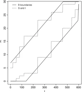
Fig. 1. Example of theMCG(SandI) andBboundaries withα=0.05 and a maximum number of simulations equal ton=600.

H_A∗

:

p

> α

(2)

wherepis the realized and unknownp-value. Viewed as a random variable, we denote thep-value byP. Clearly, the decision

in favor of any of the above hypotheses leads to a decision concerning the original hypothesesH0andHA.

Letu0be the observed value of the test statisticUbased on a fixed sample and letu1

,

u2

, . . .

be independently simulated

values fromUunderH0. Let

Xt

=

t



i=1

1_{[u0,∞)}

(

ui

),

where 1_{[u0,∞)}

(

ui

)

is the indicator function thatui

≥

u0.

[8] used theB-value introduced by [10] to propose a sequential procedure to testH₀∗versusH_A∗.

DefineV

(

t

)

=

min



x

≥

0

_:

x

−

tx

≥

c1

{

n

α(

1

−

α)

}

1/2



andL

(

t

)

=

max



x

≥

0

:

x

−

t

α

≤

c2

{

n

α(

1

−

α)

}

1/2



.

Let Bupper

=



(

t

,

x

)

=

(

t

,

min

{

V

(

t

),

r1

}

)

:

t

=

t0+

,

t0+

+

1

, . . . ,

n



be the upper boundary, and Blower

=



(

t

,

x

)

=

(

t

,

max

_{

L

(

t

),

t

₋

r0

}

)

:

t

=

t0−

,

t0−

+

1

, . . . ,

n



be the lower boundary of a sequential procedure, wheret₀+is the smaller

value oftsuch thatV

(

t

)

≤

tandt₀−is the smaller value oftsuch thatL

(

t

)

≥

0. Similarly, lett₁+be the smaller value oft

such thatV

(

t

)

_≥

r1andt1−the smaller value oftsuch thatL

(

t

)

≤

t

−

r0. The stopping boundaries from [8] are given by

B

=

Blower

∪

Bupper. TheBboundaries are formed by the union of linear functions int. Tuning parametersc1andc2were

specified by [8] using numerical calculations in order to reduce the expected number of simulations.Fig. 1illustrates with

solid lines theB-boundariesBupperandBlowerusingc1

= −

c2

=

1

.

282,n

=

600 and

α

=

0

.

05. The choice ofc1andc2here

is just following the specification used by [8]. This is one among the best choices tabled by [8] in the sense of having small

execution times.

The upper boundaryBupperis formed by the union of the lineV

(

t

)

=

c1

{

n

α(

1

−

α)

}

1/2

+

t

α

untilt

=

t1+, when the

upper boundary becomes the horizontal line with heightr1

= ⌊

α(

n

+

1

)

⌋

. The lower boundaryBloweris formed by the line

L

(

t

)

=

c2

{

n

α(

1

−

α)

}

1/2

+

t

α

up tot

=

t1−when it becomes the vertical liner0

=

t

− ⌈

(

1

−

α)(

n

+

1

)

⌉

.

The simulations are interrupted in the first time thatXtreaches one of the boundaries. [8] uses

φ

FKH, the test criterion

based on the validp-value presented in [4]. The validp-value is defined asp

_ˆ

v

(

Xt

,

t

)

=

FpˆMLE

(

Xt

/

t

)

, wherep

ˆ

MLE is the

maximum likelihood estimator ofpandFp_ˆis defined in (5.2) from [4]. The estimatep

ˆ

v

(

Xt

,

t

)

of thep-value can be computed

using the FKH algorithm. The test adopted by [8] for theBboundaries is given by:

φ

FKH

(

t

,

x

)

=



1

,

ifp

ˆ

v

(

x

,

t

)

≤

α

0

,

ifp

_ˆ

v

(

x

,

t

) > α.

When

φ

FKH

(

t

,

x

)

=

0, the hypothesisH0is not rejected, becauseH0∗

:

p

≤

α

is rejected. Henceforth, this procedure is called

MCB.

It is important to remark that there is no need to check the value ofXtat every momentt. To see this, note that the

boundariesBupperandBlowerare composed by non-integer numbers whileXt is a count. As a consequence, there will be

boundary at these times. To illustrate this, consider the boundariesBupperandBlowerbetween the times 134 and 179 in the

Fig. 1represented by the solid lines. The lower boundary is equal to zero untilt

=

136 and it is formed by numbers smaller

than 1 untilt

=

156. Therefore,Xtreaches the lower boundary during this period ifX137

=

0 and there is no need to check

against it fort

_≤

156. Likewise, ifXtis not interrupted byBloweratt

=

157 (that is, ifX157

>

2), it will not reach it at least

untilt

=

176. Therefore, in practice, there is no need to check against the lower boundary for every simulated value. One

needs to check only on those timestsuch that

⌈

Blower

(

t

−

1

)

⌉

<

⌈

Blower

(

t

)

⌉

fort

₌

t1

, . . . ,

n, wheret1is the greatest value oft such thatBlower

(

t

)

=

0. This will be explored by our generalized

sequential Monte Carlo method described in Section3.

SinceBupperwill typically be non-integer, it is always possible to define step functions equivalent to the upper boundary.

To see this, consider againFig. 1. Fromt

₌

134 tot

₌

143, the slowly increasing values ofBupper

(

t

)

could be all substituted

by 14 and the procedure would remain the same.

2.1. Bounding the resampling risk of MCB

[3] considered the IPO procedure, which adjusts an initial set of boundaries as the simulations proceeds. This method

allows the bounding of the resampling risk. The IPO procedure is not described in details here, but it should be noted that

it is a computationally intensive procedure, and its implementation is intractable for small values of resampling risk. [3]

considered a rather restrictive class ofp-value distributions, with cumulative distribution function given by:

Hα,1−β

(

p

)

=

1

−

Φ



Φ−1

(

1

−

p

)

−

Φ−1

(

1

−

α)

+

Φ−1

(β)



(3)

whereΦ

(.)

is the cumulative distribution function of a standard Normal distribution,

α

is the desired significance level and

β

is the type II error probability. When

α

=

1

−

β

, the cumulative distributionHα,1−β

(

p

)

has a uniform distribution on

(

0

,

1

)

, as is expected whenH0is true.

Thep-value distribution defined in(3)assumes a variety of shapes, but the analytical manipulation of the resampling

risk or of the expected number of simulations is intractable. To circumvent this problem, [3] used a Beta

(

a

,

b

)

distribution

to approximateHα,1−β

(

p

)

, and this approximation is denoted byH

˜

α,1−β

(

p

)

. This approximation is chosen such that the

expected value ofPcoincides with that fromHα,1−β

(

p

)

and such thatH

˜

α,1−β

(α)

=

Hα,1−β

(α)

=

1

−

β

. Numerical studies

were performed by [3] to obtain the worst caseF

˜

within the class(3)in the sense of having the largest resampling risk. Let

˜

F∗be the correspondent Beta distribution approximation toF

˜

.

AlthoughMCBis simpler and it presents a smaller expected time execution than the IPO procedure, it depends on the FKH

algorithm which requires rather complex modifications for each type of sequential design. [8] proposes an approximation

for theMCBprocedure. With this approximation, ifBupperis reached beforeBlower

,

H0∗is rejected, whileHA∗is accepted ifBlower

is reached first. The approximation may be used to gain analytic insights on the properties of theMCBprocedure or to help

on choosing the parametersc1

,

c2, andn, as well as providing an approximation for the expected number of simulations. An

undesirable characteristic of the approximatedMCBis that it is not truncated and the expected number of simulations must

be calculated letting the maximum number of simulations go to infinity. Moreover, the approximation toMCBdoes not offer

a guarantee that the type I error probability is under control for any choice ofc1andc2. For this reason, the approximated

MCBwill not be explored here.

3. Our proposed generalized truncated sequential Monte Carlo test

The analytical treatment of theMC test power function is a cumbersome task when it is based on two interruption

boundaries. The reason is that it involves the calculation of the large number of possible trajectories of the random variable

Xt responsible for the rejection ofH0. [4] present an algorithm to calculate this number, and they used this algorithm to

obtain both, the expected number of simulations and the resampling risk, for each fixedp-value. [4] emphasize that such

algorithm is valid only for the specific sequential procedure treated in that article, and adjustments are needed to use it

with other sequential designs. [8] also used that algorithm for her calculations, and the approximatedMCBis an attempt to

escape from the dependence on special algorithms.

Aiming to overcome this limitation, we propose a truncated sequential procedure with two boundaries that have the

shape of step functions. The values ofXtare checked against the upper boundary for everytwhile they are checked against

the lower boundary in an arbitrary set of predetermined discrete moments, possibly a smaller set than all integers between

1 andn. The motivation for this design, where the lower boundary monitoring is not carried out for every timet, is to allow

for the analytical treatment of the power function, to allow for the building of optimal boundaries in the sense of minimizing

the expected simulation time, and to allow for the calculation of the expected number of simulations of the sequentialMC

test for any test statistic. We also bound the resampling risk of our sequentialMCtest.

Let

η

I

=



nI

1

, . . . ,

nIk1



, withnI

j

<

nIj+1, be a set containing the moments whenXtmust be checked against the lower

boundary given by the valuesI

₌



I1

, . . . ,

Ik1



. IfX_nI

The monitoring ofXtwith respect to the upper boundary crossing is carried out at all momentst

=

1

, . . . ,

nand this

upper boundary is also a step function. Let

η

S

₌



_nS

1

, . . . ,

nSk2



, withnS

j

<

nSj+1be the jump moments for the upper boundary.

FornS

j−1

<

t

≤

nSj, the upper boundary is given bySjwheren0S

=

0 andS1

<

S2

. . . <

Sk2. LetS

=



S1

, . . . ,

Sk2



. Therefore,

the simulations are interrupted ifDt

=

1, where:

Dt

=



1

,

if (t

∈

η

IandXt

<

Ij) or

(

Xt

=

Sj, fornSj−1

<

t

≤

nSj

)

0

,

otherwise (4)

or if the number of simulations reaches a predetermined maximum equal ton.

Letxtbe the observed value of the random variableXt. Thep-value can be estimated by:

pG

=



xt

/

t

,

ifxt

=

SjandnSj−1

<

t

≤

n S j

(

xt

+

1

)/(

t

+

1

),

ifxt

<

Ijandt

=

nIj

.

(5)

We define the test decision function for this sequential test by:

φ

G

(

t

,

x

)

=



1

,

if the lower boundaryIis reached beforeSort

₌

n

0

,

if the upper boundarySis reached beforeI

.

The hypothesisH0is rejected if

φ

G

=

1 and it is not rejected if

φ

G

=

0. This sequentialMC test will be denoted byMCG.

As an example, takek1

=

k2

=

10

,

n

=

600, and consider

η

I

=

η

S

= {

20

,

50

,

79

,

119

,

239

,

359

,

459

,

539

,

569

,

600

}

.

For the lower and upper boundary values, consider the setsI

= {

0

,

1

,

2

,

3

,

9

,

15

,

20

,

24

,

27

,

29

}

andS

=



5

,

7

,

9

,

13

,

17

,

23

,

26

,

29

,

29

,

30



, respectively.Fig. 1shows these boundaries as dashed lines.

The choice of the boundaries is closely linked to the desired

α

mc, which is equal to 0.05 in this example. In Section5, we

show how to find in a simple way the optimal boundaries to minimize the expected number of simulations for any

α

mcandn.

3.1. Power and size of the MCG

In theMCGprocedure, the rejection ofH0occurs in the first momentt

=

nI_jsuch thatxt

<

Ij. The power calculation is

simpler if we merge the two sets

η

I_and

_η

S_{. Define}

_η

₌

_η

I

_∪

_η

S

_{= {}

_n

1

, . . . ,

nk

}

withk

=

#

η

. LetS′

=



S₁′

, . . . ,

S_k′



be the

upper boundary adjusted for eachni

∈

η

in the following way. Ifni

=

nSj

∈

η

S_{for somej, thenS}′

i

=

Sj. Ifni

∈

η

I

∩



η

S



c,

thenS_i′

₌

Sjwherejis such thatnSj

=

maxr



nrS

:

nSr

<

ni



. Thus, ifnimatches with some jump time in the set

η

S, thenSi′

is equal to the value inSfor the timeni. Ifniis not an element in

η

S, thenSi′is the jump value of the

η

S_{time immediately}

precedingni.

Similarly, letI′

=



I1′

, . . . ,

Ik′



be the adjusted lower boundary. That is, whenni

=

nIj

∈

η

I_{for somej, thenI}′

i

=

Ij. If

ni

∈

η

Sbutni

̸∈

η

I, thenIi′

=

Ijwherejis such thatnIj

=

maxr



nrI

:

nIr

<

ni



.

Thus, for a given value ofp

∈

(

0

,

1

)

, the power function of theMCGprocedure, is given by:

π

G

(

p

)

=

I₁′−1



x1=0

Cn1 x1p

x1

₍

₁

₋

_p

₎

n1−x1

₊

min

_{

S′₁−1,I′₂−1

_}



x1=I1′

min

_{

I₂′−x

_

1−1,n2−n1

}

y=0

Cn2−n1 y C

n1 x1p

y+x1

₍

₁

₋

_p

₎

n2−y−x1

+

k−1



j=2

minS′_j−1,I_j′₊₁−1



xj=Ij′

minI_j′₊₁−xj−1,nj+1−nj





y=0

minS′_j−1−1,xj





xj−1=I_j′₋₁

· · ·

min

{

S

_

′₁−1,x2

}

x1=I₁′

Cynj+1−njCxn11p

y+xj

₍

₁

₋

_p

₎

nj+1−y−xj

j



i=2

Cni−ni−1

x_i−x_i−1 (6)

whereCb

a

=

b

!

/

a

!

(

b

−

a

)

!

. This expression is composed byksummands. Ifkis not too large, the direct application of this

expression is simple and quick. However, for large values ofkthis calculation is computationally harder, as is the case in the

MCBprocedure, wherek

=

2

⌊

α

mcn

⌋

, especially for large values ofn, as 9999, for example.

Under the null hypothesis,Pfollows theU

(

0

,

1

)

distribution. Hence, by integrating out(6)with respect toPwith aU

(

0

,

1

)

density, we obtain the type I error probability forMCG:

P

(

type I error

)

=



1

0

π

G

(

p

)

dp

=

I₁′ n1

+

1

+

min

{

S′₁

_

−1,I₂′−1

}

x1=I′1

min

{

I₂′−x

_

1−1,n2−n1

}

y=0

Cn2−n1 y Cxn11

(

n2

+

1

)

C n2 y+x1

+

k−1



j=2

minS′_j−1,I_j′₊₁−1



xj=Ij′

minI′_j+1−xj−1,nj+1−nj





y=0

minS_j′₋₁−1,xj





xj−1=I_j′₋₁

· · ·

min

_{

_

S₁′−1,x2

}

x1=I′1

Cynj+1−njCxn11 j



i=2

Cni−ni−1 xi−xi−1



nj+1

+

1



Cyn+j+x1j

An upper boundbGfor the power difference betweenMCGand the exact test can be obtained:

bG

=

max p∈(0,1)



1(0,α]

−

π

G

(

p

)



,

(8)

where

α

is the significance level of the exact test. Observe that

α

is also implicitly the nominal significance level forMCG.

Section5.1gives the details about how to build boundaries in order to guarantee a Type I error smaller than or equal to

α

.

The power function

π

G

(

p

)

evaluated for a fixedpis equal to the probability ofXtreachingIbefore reachingS, and this

probability is decreasing withp. In this way, as compared to the exact test, the largest power loss ofMCGis given by:

bG

=

max

p∈(0,α]

{

1

−

π

G

(α)

} =

1

−

π

G

(α).

(9)

LetMCmbe the conventionalMCtest performed with a fixed numbermof simulations. An upper bound for the power

difference betweenMCmandMCGis given by:

bm,G

=

max

p∈(0,1)

{

π

m

(

p

)

−

π

G

(

p

)

}

,

(10)

where

π

m

(

p

)

=

P

(

G

≤ ⌊

m

α

mc

⌋ −

1

)

is the power function ofMCmfor a givenp, andGis distributed according to a binomial

distribution with parametersmandp.

3.2. Expected number of simulations for MCG

LetLbe the random variable that represents the number of simulations carried out until the halting moment. To perform

the computation of the expectation ofL, obtained byE

(

L

|

P

=

p

)

=



nk

l=1lP

(

L

=

l

|

P

=

p

)

, for each fixedp. The probability

P

(

L

=

l

|

P

=

p

)

forl

≤

n2is given by:

P

(

L

₌

l

_|

P

₌

p

)

₌























































































C_ll₋−_S1′ 1p

l−S₁′

₍

₁

−

p

)

S′1 _ifl

_<

_n1

C_ll₋−_S1_′

1p l−S₁′

₍

₁

−

p

)

S′1

+

I′₁−1



x=0

Cn1 x p

x

₍

₁

−

p

)

n1−x _ifl

₌

_n 1

I₁′−1



x=0

Cn1 x C

l−n1−1 l−n1−(S′2−x)p

S′₂

₍

₁

−

p

)

l−S2′ _ifn1

_<

_l

_<

_n2

I₁′−1



x=0

Cn1 x C

l−n1−1 l−n1−(S′₂−x)p

S′₂

₍

₁

−

p

)

l−S2′

+

min

_{

S₁′−1,I₂′−1

_}



x=I′₁

min

_{

I′₂−

_

x−1,n2−n1

}

y=0

×

Cn2−n1

y p y

(

1

₋

p

)

n2−n1−y_Cn1 x p

x

(

1

₋

p

)

n1−x _ifl

₌

_n 2.

Forl

₌

nj, withj

=

3

, . . . ,

k

−

1, we have:

P

(

L

₌

l

_|

P

₌

p

)

=

minS_j′₋₁−1,I′_j−1



xj−1=I_j′₋₁

minI_j′−xj−1−1,nj−nj−1





y=0

minS′_j−2−1,xj−1





xj−2=I_j′₋₂

· · ·

min

{

_

S₁′−1,x2

}

x1=I1′

Cynj−nj−1Cxn11p

y+xj−1

₍

₁

₋

_p

₎

nj−y−xj−1 j−1



i=2

Cni−ni−1 xi−xi−1

+

minS_j′₋₁−1,I′_j−1



xj−1=Ij′−1

minS_j′₋₂−1,xj−1





xj−2=Ij′−2

· · ·

min

_{

_

S₁′−1,x2

}

x1=I1′

C_nnj−nj−1−1

j−nj−1−(Sj′−xj−1)C n1 x1p

l−S_j′

(

1

₋

p

)

Sj′

j−1



i=2

Cni−ni−1 xi−xi−1

.

Fornj−1

<

l

<

nj, withj

=

3

, . . . ,

k:

P

(

L

=

l

|

P

=

p

)

=

minS′_j−1−1,I_j′−1



xj−1=I_j′₋₁

minS_j′₋₂−1,xj−1





xj−2=I_j′₋₂

· · ·

min

_{

_

S₁′−1,x2

}

x1=I1′

C_nnj−nj−1−1

j−nj−1−(Sj′−xj−1)C n1 x1p

l−S_j′

(

1

₋

p

)

Sj′

j−1



i=2

Finally, forl

₌

nk, we have:

P

(

L

=

l

|

P

=

p

)

=

minS′_j

−1−1,Ij′−1





xj−1=I′j−1

minI_j′−xj−1−1,nj−nj−1





y=0

minS_j′ −2−1,xj−1





xj−2=I′j−2

· · ·

min

_{

_

S₁′−1,x2

}

x1=I′1

Cynj−nj−1Cxn11p

y+xj−1

₍

₁

₋

_p

₎

nj−y−xj−1 j−1



i=2

Cni−ni−1

xi−xi−1

.

(11)

Using thatPhas aU

(

0

,

1

)

distribution under the null hypothesis, we have

E

(

L

|

H0is true

)

=



1

0

E

(

L

|

P

=

p

)

dp

.

(12)

To calculateE

(

L

)

underHAit is necessary to know thep-value distribution. However, a bound is easier to calculate as

bE(L)

=

max

p∈(0,1)

{E

(

L

|

P

=

p

)

}

.

(13)

The valuebE(L)is a very conservative upper bound forE

(

L

)

. However, as we will illustrate in Section5, in practical situations

it is useful to bound the expectation ofLasE

(

L

)

≤

0

.

523

(

n

+

1

)

.

4. A class of distributions for thep-value

Let the set

ℑ

be the class of probability distributions for thep-valueP. [8] showed that, forp

=

α

, the resampling risk

is at least 0.5. Hence, it is not possible to bound the resampling risk in relevant values for allPin

_ℑ

if this class includes

possible distributions. This is the reason we restrict

_ℑ

to be the set of all continuous probability distributionsfP

(

p

)

in

(

0

,

1

)

with differentiable densities that are non-increasing inp. From thep-value definition, its probability distribution function

can be written in the following way:

P

(

P

≤

p

)

=



1

−

FA



F0−1

(

1

−

p

)



,

ifUis large underHA

,

FA



F₀−1

(

p

)



,

ifUis small underHA

(14)

whereFAdenotes the probability distribution function of the test statisticUunderHAandF0is the distribution ofUunderH0.

Assuming the existence of density functionsfA

(

u

)

andf0

(

u

)

ofUunderHAandH0, respectively, thep-value density can

be written as:

fP

(

p

)

=



















fA



F0−1

(

1

−

p

)



f0



F₀−1

(

1

₋

p

)



,

ifUtends to be large underHA

,

fA



F₀−1

(

p

)



f0



F0−1

(

p

)



,

ifUtends to be small underHA

.

(15)

Hence, we can study the behavior of thep-value distribution by studying the behavior of the ratio betweenfA

(

u

)

andf0

(

u

)

.

In the majority of the real applications, the ratio(15)is non-increasing withp, and this is the motivation to restrict the

analysis of the resampling risk to the set

ℑ

. For example, suppose thatfA

(

u

)

andf0

(

u

)

belong to the same single-parameter

exponential family with parameters

θ

0and

θ

AunderH0andHA, respectively. From the expression(15), for

θ

0

≤

θ

A, the

p-value density is proportional toF0−1

(

1

−

p

)(θ

0

−

θ

A

)

, which is non-increasing withp. For

θ

0

≥

θ

A, thep-value density

is proportional toF₀−1

(

p

)(θ

0

−

θ

A

)

, which is also a non-increasing function ofp. Therefore,

ℑ

matches with a considerable

variety of real applications.

Let

_ℑ

Bbe the class ofp-value distributions defined in [3] with cumulative distributionHα,1−β

(

p

)

, as described in Section2.

Let

π

be the power of the exact test. We will show now that, for unbiased tests (that is, with

π

≥

α

),

ℑ

is more general

than

_ℑ

B.

From the expression(3), the densitiesh

(

p

)

∈ ℑ

Bcan be indexed by

α

and

β

and they are given by:

hα,1−β

(

p

)

=

exp



−

1₂



Φ−1

(β)

₋

Φ−1

(

1

₋

α)

 

Φ−1

(β)

₋

Φ−1

(

1

₋

α)

₊

2Φ−1

(

1

₋

p

)





(16)

whereΦ−1is the inverse function of the standard normal cumulative distribution functionΦ

(

·

)

. The first derivative of

hα,1−β

(

p

)

with respect topis equal to:

h′_α,1−β

(

p

)

=



Φ−1

(β)

−

Φ−1

(

1

−

α)



where

φ(

_·

)

is the density function of the standard normal distribution. For 1

₋

β

_≥

α

, we haveh′_α,1−β

(

p

)

_≤

0 for all p

∈

(

0

,

1

)

.

Consider the subset of densities

_ℑ

∗

B

= {

fP

(

p

)

∈ ℑ

B

:

1

−

β

≥

α

}

. That is,

ℑ

∗Bis a subset from

ℑ

Bformed only by densities

that implies unbiased tests. Therefore,

ℑ

∗

B

⊂ ℑ

. Thus, the class

ℑ

Bis a particular case from

ℑ

in the class of unbiased tests.

Since biased tests are typically useless, we proved that our class is larger than

ℑ

Bin all relevant cases.

Furthermore, the class

_ℑ

Bdoes not cover all cases of interest. For example, the spatial scan statistic developed by [9] to

detect spatial clusters follows very closely a Gumbel distribution under the null hypothesis and a chi-square distribution

underHA[1]. Therefore, even in interesting applied situations, there is not guarantee thatfP

(

p

)

∈ ℑ

Band a larger class, such

as ours, may be useful.

There is another example where we can show analytically that

_ℑ

Bis too restrict for practical purposes. For 1

−

β

≥

α

andp

_≤

0

.

5, the densityhα,1−β

(

p

)

∈ ℑ

Bis a convex function. To see this, it is enough to show that its second derivative

with respect topis positive. Since

h′′_α,1−β

(

p

)

=



Φ−1

(β)

−

Φ−1

(

1

−

α)

−

φ

′

(

Φ−1

(

1

−

p

))



φ(

Φ−1

₍

₁

₋

_p

₎₎

h

′

α,1−β

(

p

)

(18)

and we have that

φ

′

(

Φ−1

(

1

−

p

))

=

Φ

−1

₍

₁

−

p

)

√

2

π φ(

Φ−1

₍

₁

₋

_p

₎₎

exp



−

1

/

2



Φ−1

(

1

−

p

)



2



≥

0

ifp

_≤

0

.

5, we conclude thath′′

α,1−β

(

p

)

≥

0. However, in many practical cases, the densityhα,1−β

(

p

)

∈ ℑ

Bis not a convex

function. For example, supposeU0

∼

χ

12

(

0

)

andUA

∼

χ

12.01

(

0

)

. The correspondingp-value density from this conjecture is

not convex forp

>

0

.

32.

Our more general

_ℑ

family is not restricted to families such as the normal, chi-square orFdistributions. It also contains

p-value densities with mixed shapes, with concave and convex parts. However, it is important to point out that the class

ℑ

is

not required to use ourMCGprocedure. In particular, we do not need this class to calculate a bound for the power loss with

respect to theMCmor to the exact test. We do not need this class either to establish the bound for the expected number of

simulations underHA. The results in Sections3.1and3.2are valid for any test statistic.

When the additional assumption that thep-value densityfP

(

p

)

belongs to

ℑ

holds, stronger results can be obtained. In

the next subsections, we show that assuming

_ℑ

allows the bounding of the resampling risk in a very simple way, as well as

to obtain better results for the power and the expected number of simulations of our generalized Monte Carlo test procedure

than those in Section3.

4.1. Upper bound for the power difference between the exact test and MCG

The power of the generalized Monte Carlo test is given by integrating out the probability

π

G

(

p

)

of rejecting the null

hypothesis conditioned on thep-valuepwith respect to thep-value density:

π

G

=



1

0

π

G

(

p

)

fP

(

p

)

dp

.

(19)

The power difference between the exact test andMCGis given by:

δ

G

=



1

0



1(0,αmc]

(

p

)

−

π

G

(

p

)



fP

(

p

)

dp

.

(20)

An upper boundb∗_Gfor the power loss

δ

Gcan be obtained if we take the worst possible case forfP

(

p

)

. That is, assume that the

p-value density is given byfP,w

(

p

)

=

1

/α

mc, ifp

∈

(

0

, α

mc

]

, and byfP,w

(

p

)

=

0, otherwise. Therefore, the bound is given by

b∗_G

=



1

0



1(0,αmc]

(

p

)

−

π

G

(

p

)



fP,w

(

p

)

dp

=



αmc

0

1

α

mc

dp

−



αmc

0

π

G

(

p

)

1

α

mc

dp

=

1

₋

1

α

mc



αmc

0

π

G

(

p

)

dp

.

(21)

Because the function(6) is a sum of Beta

(

a

,

b

)

density kernels, the integral(21)can be rewritten as a function of

incomplete Beta

(

a

,

b

)

functions, all of them evaluated atp

₌

α

mc, withaandbdepending only of the parametersI

,

S

and

η

. In the same way, an upper bound for the power difference betweenMCmandMCGis given by:

b∗_m,G

₌



αmc

0

(π

m

(

p

)

−

π

G

(

p

))

1

α

mc

dp

.

(22)

4.2. An upper bound for the expected number of simulations

For values ofpnear 0, the simulation time is aroundn1, the first checking point of the lower boundary in the sequential

procedure. For values ofpnear 1, the simulation time is aroundS₁′, the smallest height of the upper boundary. Numerically,

we find thatE

(

L

_|

P

₌

p

)

is maximized forparound

α

mc. Let

pmax

=

arg max

p E

(

L

|

P

=

p

)

and definef

¯

P,max

(

p

)

=

1

/

pmax, forp

∈

(

0

,

pmax

]

, and

¯

fP,max

(

p

)

=

0, otherwise. Thus, it follows that

E

(

L

)

=



1

0

E

(

L

|

P

=

p

)

¯

fP

(

p

)

dp

≤



1

0

E

(

L

|

P

=

p

)

f

¯

P,max

(

p

)

dp

=



1/pmax

0

E

(

L

|

P

=

p

)

1 pmax

dp

.

(23)

The right hand side of the inequality(23)defines an upper boundb∗_E(L)forE

(

L

)

.

4.3. An upper bound for the resampling risk

LetRRbe the resampling risk in aMCtest defined as:

RR

=

Pmc

(

H0is not rej.

|

P

≤

α)

P

(

P

≤

α)

+

Pmc

(

H0is rej.

|

P

≥

α)

P

(

P

≥

α)

(24)

wherePmcis the probability measure associated with the events generated byMCsimulations. For theMCGtest, denote its

resampling risk byRRG, which is computed as:

RRG

=



α

0

[1

−

π

G

(

p

)

]fP

(

p

)

dp

+



1

α

π

G

(

p

)

fP

(

p

)

dp

.

(25)

As

π

G

(

p

)

is a decreasing function ofp, the function 1p∈(0,α]

(

p

)

−

π

G

(

p

)

is maximum atp

=

α

. Thus,RRGis maximum when

fP

(

p

)

puts the largest possible mass at

α

, which is the worst casefP,w

(

p

)

. SubstitutingfP

(

p

)

in(25)byfP,w

(

p

)

and setting

α

₌

α

mc, we have:

RRG

≤

1

−

1

α

mc



αmc

0

π

G

(

p

)

dp

.

(26)

Therefore, an upper bound forRRGis equal to the upper bound(21)for the power loss with respect to the exact test. That is,

b∗_RR

G

=

b

∗

G.

Recall that

π

is the power of the exact test and

π

Gis the power of the generalized sequential test calculated as shown in

(19). The expression(25)can be rewritten in a way that emphasizes another property. When

π < π

Gwe should obviously

prefer the sequential test and there would be issue concerning the resampling risk. Therefore, the control ofRRGis important

only when

π

≥

π

G. This inequality implies thatRRG

≥

δ

G, where

δ

Gis the power difference between the exact test andMCG.

Therefore, equal power of the exact test and theMCGtest does not imply a null resampling risk. To see this, note that:

RRG

=



αmc

0

fP

(

p

)

dp

−



αmc

0

π

G

(

p

)

fP

(

p

)

dp

+



1

αmc

π

G

(

p

)

fP

(

p

)

dp

=

π

−

π

G

+

2



1

αmc

π

G

(

p

)

fP

(

p

)

dp

=

δ

G

+

2



1

αmc

π

G

(

p

)

fP

(

p

)

dp

.

(27)

5. Optimal boundaries

This section presents a constructive way to find theMCGoptimal in the sense of minimizing the expected number of

simulations among all the procedures controlling the sequential risk. LetRS

(

t

|

H0

)

be the sequential risk associated with the

upper boundarySdefined as theH0probability that the sequential test do not reject the null hypothesis attand the fixed

mconventional MC test does rejectH0. That is,

RS

(

t

|

H0

)

=

P

(

Xt

≥

Sj

,

Xm

<

⌊

α

mc

(

m

+

1

)

⌋ |

H0

)

=

x0



x=Sj

y0



y=0