Scale-Adjusted Metrics for Predicting the
Evolution of Urban Indicators and
Quantifying the Performance of Cities
Luiz G. A. Alves1,2, Renio S. Mendes1,2, Ervin K. Lenzi1,2,3, Haroldo V. Ribeiro1,4*
1Departamento de Física, Universidade Estadual de Maringá, Maringá, PR 87020-900, Brazil,2National Institute of Science and Technology for Complex Systems, CNPq, Rio de Janeiro, RJ 22290-180, Brazil,
3Departamento de Física, Universidade Estadual de Ponta Grossa, Ponta Grossa, PR 84030-900, Brazil,
4Departamento de Física, Universidade Tecnológica Federal do Paraná, Apucarana, PR 86812-460, Brazil
Abstract
More than a half of world population is now living in cities and this number is expected to be two-thirds by 2050. Fostered by the relevancy of a scientific characterization of cities and for the availability of an unprecedented amount of data, academics have recently immersed in this topic and one of the most striking and universal finding was the discovery of robust allometric scaling laws between several urban indicators and the population size. Despite that, most governmental reports and several academic works still ignore these nonlineari-ties by often analyzing the raw or the per capita value of urban indicators, a practice that actually makes the urban metrics biased towards small or large cities depending on whether we have super or sublinear allometries. By following the ideas of Bettencourtet al.[PLoS ONE 5 (2010) e13541], we account for this bias by evaluating the difference between the actual value of an urban indicator and the value expected by the allometry with the popula-tion size. We show that this scale-adjusted metric provides a more appropriate/informative summary of the evolution of urban indicators and reveals patterns that do not appear in the evolution of per capita values of indicators obtained from Brazilian cities. We also show that these scale-adjusted metrics are strongly correlated with their past values by a linear corre-spondence and that they also display crosscorrelations among themselves. Simple linear models account for 31%–97% of the observed variance in data and correctly reproduce the average of the scale-adjusted metric when grouping the cities in above and below the allo-metric laws. We further employ these models to forecast future values of urban indicators and, by visualizing the predicted changes, we verify the emergence of spatial clusters char-acterized by regions of the Brazilian territory where we expect an increase or a decrease in the values of urban indicators.
OPEN ACCESS
Citation:Alves LGA, Mendes RS, Lenzi EK, Ribeiro HV (2015) Scale-Adjusted Metrics for Predicting the Evolution of Urban Indicators and Quantifying the Performance of Cities. PLoS ONE 10(9): e0134862. doi:10.1371/journal.pone.0134862
Editor:Celine Rozenblat, University of Lausanne, SWITZERLAND
Received:February 5, 2015
Accepted:July 14, 2015
Published:September 10, 2015
Copyright:© 2015 Alves et al. This is an open access article distributed under the terms of the Creative Commons Attribution License, which permits unrestricted use, distribution, and reproduction in any medium, provided the original author and source are credited.
Data Availability Statement:All data are maintained and made freely available by the Department of Informatics of the Brazilian Public Health System. Brazil’s Public healthcare System (SUS), Department of Data Processing (DATASUS), 2011. Available: http://www.datasus.gov.br/. Date of access: 01 2015 Jan.
Introduction
Over the past six decades the world went through a period of quick and remarkable urbaniza-tion. According to the United Nations [1] in the year of 2007, for the first time, the world urban population has surpassed the rural one and, if this process persists, two-thirds of the world population are expected to be living in urban areas by 2050. On one hand, cities are usu-ally associated with higher levels of literacy, health care and better opportunities; on the other hand, unplanned urbanization and bad political decisions also lead to pollution, environmental degradation, growth of crime, unequal opportunities and the increase in the number of people living in substandard conditions. In this sense, there is a vast necessity for finding patterns, quantifying and predicting the evolution of urban indicators, since these investigations may provide guidance for better political decisions and resources allocation.
Fostered by this need and also due the availability of an unprecedented amount of data at city level, several researchers have recently promoted an impressive progress into what has been calledScience of Cities[2]. These new data allowed researchers to probe patterns of the cities to a degree not before possible and one of the most striking and universal finding of these studies was the discovery of robust allometric scaling laws between several urban indicators and the population size. Patents, gasoline stations, gross domestic product [3–6], carbon emis-sions [7,8], crime [6,9–14], indicators of education [13], suicides [15], number of election can-didates [16,17], transportation networks [18,19], employees from several sectors [20],
measures of social interaction [21] are just a few examples where robust scaling laws have been found. Despite these intrinsic nonlinear relationships it is common to find works that try unveiling relationships between population size and urban indicators by employing linear regressions in the raw data; also, per capita indicators (that is, divided by population size) are ubiquitous in reports of government agencies and are often used as a guide for public policies when analyzing the temporal evolution of a given city or for comparing/ranking the perfor-mance of cities with different population sizes. However, these linear regressions may result in misguided/controversial relationships [11,22] and per capita indicators are oblivious to the allometric scaling laws that make city a complex agglomeration that cannot be modeled as a linear combination of its individual components [6,23,24]. In this sense, there is a paucity of alternative metrics for urban indicators that may overcome the foregoing problems and pro-vide a fairer comparison between cities of different sizes as well as a better understanding of the city evolution. Bettencourtet al.[6] have recently proposed a simple alternative to overcome these nonlinearities by evaluating the difference between the actual value of the urban indica-tors and the value expected by the allometries with the population size (that is, the residuals in the allometric relationships). This scale-adjusted metric explicitly considers the allometric rela-tionships and already have proved to be useful in the economic context [25,26] and for unveil-ing relationships between crime and urban metrics that are not properly carried out by regression analysis [11].
In this article, we follow the evolution of this relative metric for eight urban indicators from Brazilian cities in three years (1991, 2000 and 2010) in which the national census took place. By grouping cities in above and below the allometric laws, we argue that the average of this scale-adjusted metric provides a more appropriate/informative summary of the evolution of the urban indicators when compared with the per capita values; it also reveals patterns that do not appear when analyzing only the evolution of the per capita values. For instance, while the per capita values of homicides have systematically increased over the last three decades, both the average of the scale-adjusted metric for cities above and below the allometric law are approaching zero, that is, cities where the number of homicides is above the expected by the allometry have managed to reduce this crime, whereas this crime has been increased in those
and RSM thanks FA (grant 263/2014) for partial financial support. The funders had no role in study design, data collection and analysis, decision to publish, or preparation of the manuscript.
cities where number of homicides is below the allometry. We argue that the nonlinearities may affect the per capita indicators by creating a bias towards large cities for superlinear allometries and a bias towards small cities for sublinear allometries. We further show that these scale-adjusted metrics are strongly correlated with their past values by a linear correspondence, mak-ing them particularly good for predictmak-ing future values of urban indicators through linear regressions. We have tested this hypothesis via a linear model where the scale-adjusted metric for one indicator in a given census was predicted by a linear combination of all eight metrics evaluated from the preceding census. These simple models account for 31%–97% of the observed variance in data and correctly reproduce the average value of the scaled-adjusted met-ric when grouping the cities in above and below the allometmet-ric laws. Motivated by these good agreements, we present a prediction for the values of urban indicators in the year of 2020 by assuming the linear coefficients constants over time. By visualizing the predicted changes, we verify the emergence of spatial clusters characterized by regions of the Brazilian territory where the model predicts an increase or a decrease in the values of urban indicators. We further report a list containing all the scale-adjusted metrics as well as the predictions for each city in the hope that government agencies find these informations useful (S1 Dataset).
Results and Discussion
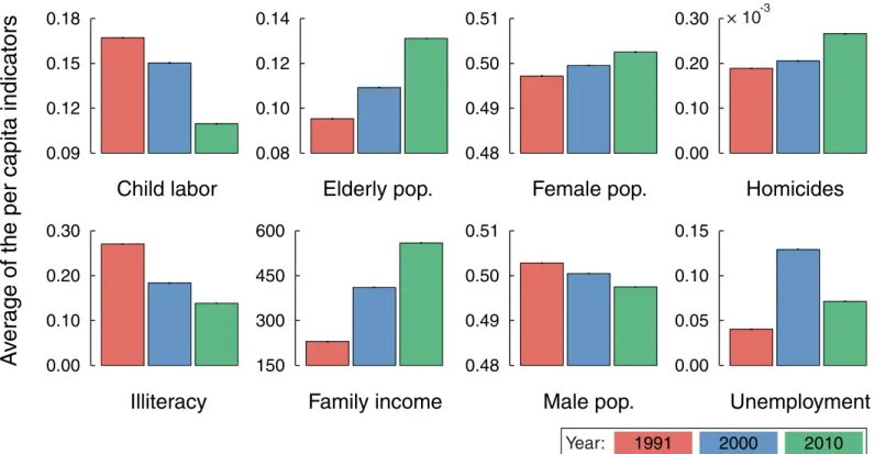
We start by considering the average of the per capita values for eight urban indicators described in the Methods Section. This is a common practice of government agencies for tracking the evolution of a particular city or for comparing a group of cities with different populations. We observe inFig 1that almost all per capita indicators show a clear temporal trend: elderly popu-lation, female popupopu-lation, homicides and family income have increased over the years; whereas child labor, illiteracy and male population have decreased (the unemployment rates have evolved in a more complex manner, exhibiting no clear tendency). We could also list the cities in which these indicators have considerably changed or rank the cities that have made more progress in reducing, for instance, the homicide or illiteracy rates.
One of the main problems with this analysis is that it completely ignores the hypothesis that most urban indicatorsYi(t) displays allometric relationships (or scale invariance) with the
pop-ulationN(t), that is,
YiðtÞ ¼10
Ai
NðtÞbi; ð1Þ
whereAiis a constant,βiis the allometric (or scaling) exponent andtstands for time. This
sim-ple relationship summarizes the (average) effects of increasing the population size on the urban indicators; it states that cities are self-similar in terms of their population, in the sense that average properties of a given city can be inferred only by knowledge of its population. Urban indicators are thus expected to display a deterministic component emerging from very few and general properties of the urban networks related to social and infrastructure aspects of cities [24]. When analyzing per capita values, it is implicitly assumed that the value of an urban indicator is proportional to the population size (βi= 1) or, in other words, that cities are exten-sive systems. This idea is opposed to the complex systems approach of cities: complex systems are non-extensive (βi6¼1), meaning that its isolated parts do not behave in the same manner as when they are interacting. Cities have similar properties and only make sense as an entire
indicators, often resulting in per capita savings of material infrastructure and in gain of socio-economic productivity [3]. From a more technical point of view, whenever the allometric expo-nentβiis different from one, there is a remaining component related to the population size when evaluating the per capita values of these urban indicators, that is,yi=Yi/N*N(βi−1),
which creates a bias towards large cities forβi>1 and towards small cities forβi<1; per capita measures are only efficient in correctly removing the effect of the population size in an urban indicator forβi= 1. For our data, a complete description of the allometric relationships between the eight urban indicators and the population is presented in the Methods Section, where we have confirmed the presence of allometries in our data as summarized inTable 1(see alsoS1 andS2Figs).
The problem with per capita indicators thus prompts the question on how we can account for these allometries and correctly remove the effect of the population size on the urban indica-tors. Bettencourtet al.[6] have proposed a simple and efficient procedure for overcoming this problem by defining the so-calledscale-adjusted urban indicator. The approach consists in evaluating the logarithmic difference between the actual value of an urban indicatorYi(t) and
the value expected by allometric relationship with the populationN(t) (that is, the residuals in the allometric relationships) in given yeart, namely,
DYiðtÞ ¼ logYiðtÞ ½Aiþbi logNðtÞ: ð2Þ Fig 1. Trends in the evolution of per capita values of Brazilian urban indicators.The bar plots show the temporal evolution of eight urban indicators in the years 1991, 2000 and 2010 in which the national census took place. The bar plots are average values over Brazilian cities, where each urban indicator for each city have been divided by the corresponding city population, that is, made per capita. The definition of each indicator is provided in the Methods Section. The tiny error bars are 95% bootstrap confidence intervals for the average values. We note that elderly population, female population, homicides and family income display an increasing tendency; whereas child labor, illiteracy and male population have decreased over time. Despite having increased, the unemployment rates show a not very clear trend.
The previous quantity explicitly considers the allometry between an urban indicator and the population size, creating a relative measure that is not biased by the population size (size-inde-pendent) for any value ofβi. The scale-adjusted metricDYi(t) captures the exceptionality (either good or bad) of a city, which somehow is the result of the nonlinear agglomeration process Table 1. Allometric relationships between urban indicators and population size.Values of parametersAiandβiobtained via orthogonal distance
regression on the relationship between logYi(t) and logN(t) for each urban indicator in the yeart(seeMethodsSection). The values inside the brackets are
the standard errors (SE) in the last decimal of the estimated parameters. The last column shows the values of the Pearson linear correlation coefficientρfor each allometry in log-log scale.
IndicatorYi(t) Yeart Ai(SE) βi(SE) ρ
Child labor 1991 −0.64 (5) 0.96 (1) 0.909
2000 −0.55 (5) 0.93 (1) 0.906
2010 −0.80 (5) 0.95 (1) 0.884
Elderly population 1991 −0.99 (5) 0.992 (6) 0.976
2000 −0.83 (2) 0.969 (5) 0.980
2010 −0.72 (2) 0.963 (5) 0.982
Female population 1991 −0.367 (3) 1.014 (1) 1.000
2000 −0.361 (2) 1.013 (1) 1.000
2010 −0.355 (2) 1.012 (1) 1.000
Homicides 1991 −5.4 (1) 1.35 (3) 0.769
2000 −5.7 (1) 1.41 (2) 0.800
2010 −5.04 (9) 1.29 (2) 0.827
Illiteracy 1991 −0.29 (7) 0.92 (2) 0.789
2000 −0.26 (7) 0.87 (2) 0.774
2010 −0.28 (7) 0.85 (2) 0.749
Family income 1991 0.82 (6) 0.33 (1) 0.428
2000 1.14 (6) 0.31 (1) 0.440
2010 1.63 (5) 0.23 (1) 0.440
Male population 1991 −0.239 (3) 0.987 (1) 1.000
2000 −0.243 (2) 0.987 (1) 1.000
2010 −0.249 (2) 0.988 (1) 1.000
Unemployment 1991 −3.50 (8) 1.45 (2) 0.880
2000 −2.07 (5) 1.25 (1) 0.940
2010 −2.09 (5) 1.20 (1) 0.931
doi:10.1371/journal.pone.0134862.t001
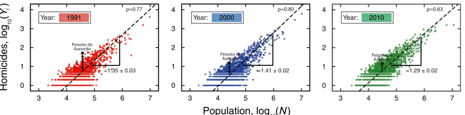
Fig 2. Allometric laws and the definition of the scale-adjusted metricDYi(t).The scatter plots show the allometric relationships between number of
homicides and population size for the yearst= 1991, 2000 and 2010 in log-log scale (seeS1andS2Figs for all other indicators). The allometric exponentsβi
(seeMethodsSection for details on the calculation ofβi) and Pearson correlation coefficientρare shown in the figures. We highlight a particular city (Peixoto
de Azevedo) in the three years to illustrate the definition and the evolutionDYi(t). For this city, the number homicides was quite above the allometric law in the
yeart= 1991; however, it has approached the expected value by the allometric law over the years.
related to the socio-economic choices and historical path of a city [6]. Furthermore,DYi estab-lish a more“natural”scale for ranking cities by identifying whether an urban indicator of a given city is above (DYi>0) or below (DYi<0) the expected value from cities of similar sizes. This approach already have proved to be useful in the economic context [25,26] and was also employed for unveiling relationships between crime and urban metrics that are not properly carried out by linear regression analysis [11].Fig 2illustrates the definition ofDYi(t) and shows an example of allometry between homicides and population size (see alsoS1andS2Figs for all urban indicators).
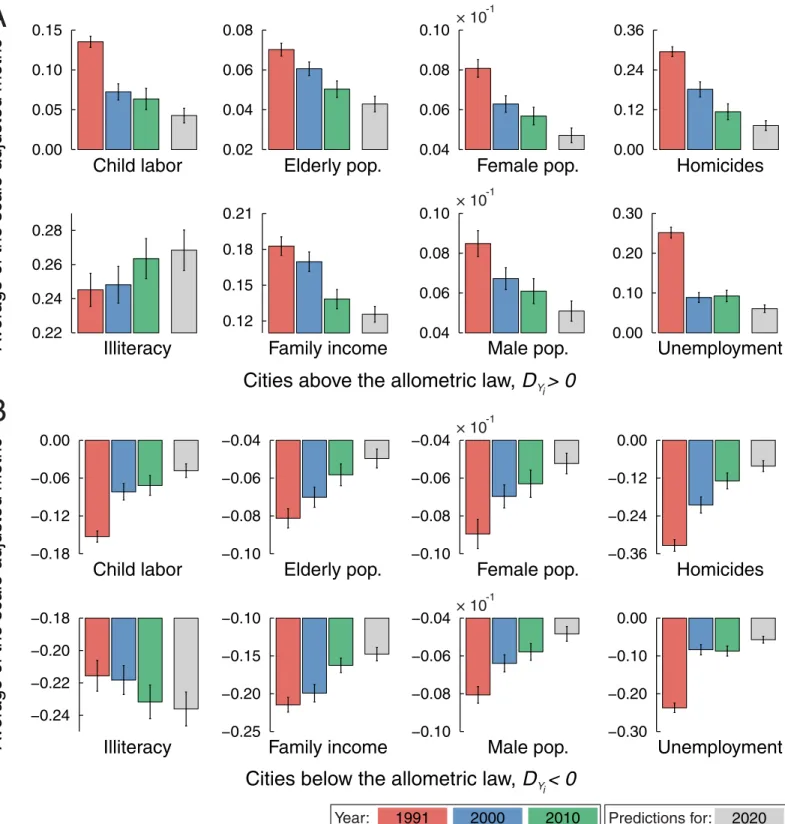
In order to show the informations that this scale-adjusted metric provides, we study the evo-lution of the averageDYi(t) by creating two groups of cities: those whose the urban indicator
Yi(t) was above (DYi(t)>0) and those whoseYi(t) was below (DYi(t)<0) the allometric law in the yeart= 1991.Fig 3shows these averages for the eight urban indicators over the three years in our database. For the majority of the urban indicators, the averageDYi(t) displays a statisti-cally significant decreasing tendency for cities initially above the allometric law; whereas an increasing tendency for the averageDYi(t) is observed for those cities that were initially below the allometric law. For instance, cities where the number of children laboring, homicides and unemployment were above the value expected by the allometric law have been successful (on average) in reducing them; in contrast, cities where these indicators were below the allometric laws proved unable (on average) to improve or maintain this situation. The case of illiteracy is an exception to the previous pattern, since the averageDYi(t) has increased for cities initially above the allometric law and it is almost a constant for those cities initially below. Thus, cities where illiteracy was initially above the allometric law have failed (on average) in increasing the number of literates; on the other hand, those cities initially below the allometric law have not only kept this feature (on average) but also managed to further improve the literacy levels. In the case of population metrics, particularly regarding female and male populations, the approaching to the allometric laws (together with the decrease in proportion of males in the population) may represent a good aspect with respect to reduction of violence, since an exces-sive contingent of men can drive an increase in antisocial behavior [29]; moreover, both male population above and female population below the allometric law correlate with number of homicides above the allometric law [11]. Similarly, family income above the allometric law cor-relates with homicides above, while family income below the allometric law corcor-relates with homicides below [11]. Remarkably, these informations remain hidden or distorted when we look only at the per capita values of these urban indicators.
The trends in the average values of the scale-adjusted metrics prompt the question of how the values of this relative metric are affected by their previous values, that is, are the values of
DYi(t+Δt) andDYi(t) correlated in some particular fashion? To answer this question, we ana-lyze the scatter plots of the scale-adjusted metric in a given year versus its past values for each urban indicator for all cities.Fig 4shows these scatter plots considering the values ofDYi(2010) versusDYi(2000) andS3 Figshows the plots forDYi(2000) versusDYi(1991). We observe that, despite the different scattering degrees (Pearson correlation ranging from 0.47 to 0.98), linear functions are good approximations for the average tendency of these relationships. We thus adjust the linear model
DYiðtþDtÞ ¼AiþaiDYiðtÞ ð3Þ
to each urban indicator via least square method and the bestfitting parameterαi(Pearson
cor-relations as well) is shown inTable 2for the two combinations of years. We have omitted the values ofAibecause they are very small (*10−6). Despite the increasing tendency observed for
Fig 3. Trends in the evolution of the average values of the scale-adjusted metrics.The bar plots show the evolution of the averageDYi(t) when grouping the cities whose urban indicator was (A) above and (B) below the allometric law in the yeart= 1991. The colorful bars are empirical data (red fort= 1991, blue fort= 2000 and green fort= 2010) and gray bars represent the predictions obtained from the linear model ofEq 6(see discussion in main text). The error bars are 95% bootstrap confidence intervals for the average values. Note that the averageDYi(t) displays a statistically significant decreasing tendency for cities whose urban indicator was initially above the allometric law and an increasing tendency is observed for cities whose urban indicator was initially below the allometric law. The only exception to this pattern is the case of illiteracy, where the averageDYi(t) has increased for cities initially above the
allometric law and it is almost a constant for those cities initially below. We further observe that the predicted values (gray bars) keep this main tendency.
1 for almost all urban indicators except for illiteracy (αi= 1.01 ± 0.01 for 2000 versus 1991 and
αi= 1.05 ± 0.01 for 2010 versus 2000). These results agree with the evolution of the average
DYi(t), that is, indicators characterized byαi<1 present a tendency of approaching the allome-tric laws, while forαi1 there should be a departing tendency from the allometric laws.
In order to better understand the role of the parameterαi, we consider the limit whereΔtis small to rewriteEq 3as the following differential equation
d
dtDYiðtÞ ¼Aiþ ðai 1ÞD
YiðtÞ; ð4Þ
Fig 4. Memory effects in the evolution of the scale-adjusted metricDYi(t).The purple dots show the values ofDYi(2010) versusDYi(2000) for each city
(seeS3 FigforDYi(2000) versusDYi(1991)). Despite the different scattering degrees (see the value of Pearson correlation coefficientρin the plots), we
observe a linear correspondence betweenDYi(2010) andDYi(2000). The dashed lines are fits of the linear modelDYi(2010) =Ai+αiDYi(2000) (Eq 3) obtained via ordinary least-square regression. The values ofαiand their standard errors are shown in the plots and also summarized inTable 2. We note thatαi<1 for
almost all indicators, a fact that is in agreement with the approach to allometric laws observed for the averages value ofDYi(t) (Fig 3). Illiteracy is the only
exception whereαi≳1. This result also agrees with the departing from the allometric law of the averageDYi(t) in the case of illiteracy.
whose solution is
DYiðtÞ ¼
Ai=ð1 aiÞ þ ½k Ai=ð1 aiÞexp½ ð1 aiÞt ðfor a6¼1Þ;
Aitþk ðfor a¼1Þ;
(
ð5Þ
wherekis an integration constant. Thus,Eq 5predicts thatDYi(t) will exponentially approach the valueAi/(1−αi) forαi<1 and that they will exponentially increase over time whenαi>1.
Forαi= 1 we have a linear behavior for the evolution ofDYi(t). It is worth remembering thatAi is a very small number (*10−6) for all urban indicators and hence the values ofDYi(t) are actu-ally approaching zero forαi<1 (that is, the values of the urban indicators are getting closer to value expected by the allometric law). We further observe that 1/(1−αi) plays the role of a
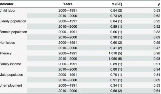
characteristic time and if we assumeαi<1, the smaller the value ofαiis, the faster we expect to be changes in the urban indicator. For population-related indicators, we observe an increasing tendency in the values ofαiand also that these values are among the largest ones, which agrees with the reduction of the Brazilian population growth in the last decades. For socio-economic indicators, we have, on one hand, that the values ofαifor child labor and unemployment have also increased (pointing out to slowdown of their dynamics); on the other hand, homicides and family income had their values ofαireduced, suggesting that their rates of change have increased. Apart from the evolution in the values ofαi, population-related indicators have (in
general) larger values ofαithan those observed for socio-economic indicators, indicating that these latter are more susceptible to natural or public policies driven changes. The illiteracy is unique because its value ofαi, that was very close to one (forDYi(2000) versusDYi(1991)), has increased, a result that agrees with the detachment from the allometry reported inFig 3and suggests an acceleration in this process.
Table 2. Linear coefficientsαiof the memory relationships between the scale-adjusted metrics in
dif-ferent years.Values of the parametersαiobtained via least square fitting the model of theEq 3for the
rela-tionships between the scale-adjusted metrics:DYi(2000) versusDYi(1991) andDYi(2010) versusDYi(2000). We have omitted the values of the parametersAibecause they are very small (*10−6). The values inside the
brackets are the standard errors (SE) in the last decimal of the estimated parameter. The last column shows the values of the Pearson linear correlation coefficientsρfor each relationship.
Indicator Years αi(SE) ρ
Child labor 2000—1991 0.54 (2) 0.53
2010—2000 0.73 (2) 0.62
Elderly population 2000—1991 0.84 (1) 0.92
2010—2000 0.89 (1) 0.92
Female population 2000—1991 0.66 (1) 0.83
2010—2000 0.90 (1) 0.89
Homicides 2000—1991 0.60 (2) 0.59
2010—2000 0.41 (2) 0.47
Illiteracy 2000—1991 1.010 (5) 0.98
2010—2000 1.050 (5) 0.98
Family income 2000—1991 0.89 (1) 0.91
2010—2000 0.80 (1) 0.94
Male population 2000—1991 0.70 (1) 0.84
2010—2000 0.91 (1) 0.89
Unemployment 2000—1991 0.34 (1) 0.53
2010—2000 0.68 (2) 0.64
In addition of being autocorrelated with their past values,DYi(t+Δt) for the urban indicator
ialso displays statistically significant crosscorrelations withDYj(t) for other indicatorsj(S4 Fig). These memory effects and also the fact that the residuals surrounding the relationships
DYi(t+Δt) versusDYi(t) are very close to Gaussian distributions (S5 Fig) with standard devia-tions across windows practically constant (S6 Fig) make these scale-adjusted metrics particu-larly good for being used in linear regressions aiming forecasts. We have thus adjusted the linear model (via ordinary least-squares method)
DYiðtþDtÞ ¼C0þ
X
8
k¼1
CkDYkðtÞ þZiðtÞ ð6Þ
by considering the relationships (t+Δt) = 2000 versust= 1991 and (t+Δt) = 2010 versus
t= 2000. InEq 6,Ckis the linear coefficient quantifying the predictive power ofDYk(t) onDYi(t +Δt) (C0is the intercept coefficient) andηi(t) is the noise term accounting for the effect of
unmeasurable factors. The results exhibiting the linear coefficients of each linear regression for the two combinations of years are shown inS1 Text. We note that these simple models account for 31%–97% of the observed variance inDYi(t+Δt) and that they correctly reproduce the aver-age values of the scale-adjusted metric above and below the allometric laws for the years 2000 and 2010 only using data from the years 1991 and 2000, respectively (seeS7 Fig). We have fur-ther compared the distributions of the empirical values ofDYiwith the predictions of these lin-ear models and observed that the agreement is remarkable good for the indicators elderly, female and male population as well as for illiteracy and income (S8andS9Figs). Motivated by these good agreements, we proposed to forecast the values ofDYi(t+Δt) in the year of 2020 (next Brazilian national census). In order to do so, we have considered that the linear coeffi -cientsCkare constant over time and employed the average value ofCkover the two
combina-tions of years used inEq 6for predicting the values ofDYi(t+Δt). It is worth noting that by assumingCkconstant, we are ignoring the evolution of socio-economic and policy factors. In
an ideal scenario, one could track the evolution of the values ofCkfor achieving more reliable
predictions. However, our data (that is, the two values forCk) do not enable us to probe
possi-ble evolutionary behaviors in the values ofCk. Even so, as pointed by Bettencourt [6], the
dynamics of the urban metrics seems to be dominated by long timescales (*30 years), and thus the approach of constant coefficients should be seen as afirst approximation. The grays bars inFig 3show the averagesDYi(2020) after grouping the cities withDYi(1991)>0 and
DYi(1991)<0. We observe that predictions for the average values basically keep the trends sented in the previous years; for unemployment, in which the trend was not very clear, the pre-dictions put this indicator together with most indicators, where the averageDYi(t) has been decreasing for cities initially above the allometric law and increasing for those initially below.
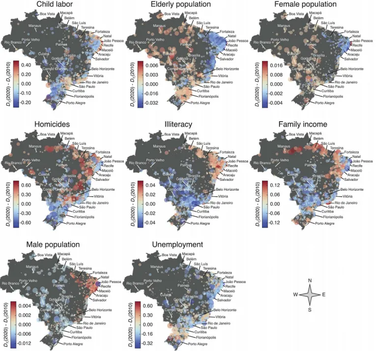
In order to gain further information on the predictions, we build a geographic visualization of the expected changes inDYi(t) between the yearst= 2010 andt= 2020. The circles over the maps inFig 5show the geographic location of Brazilian cities; the radii of these circles are pro-portional tojDYi(2020)−DYi(2010)jand are colored with shades of azure for cities where [DYi(2020)−DYi(2010)]<0 (the indicator is expected to decrease) and with shades of red for cities where [DYi(2020)−DYi(2010)]>0 (the indicator is expected to increase); in both cases, the darker the shade, the larger is the absolute value of the difference [DYi(2020)−DYi(2010)]. Perhaps, the most striking feature of these visualizations is the fact that the predicted changes appear spatially clustered for almost all indicators, which somehow reflects the geographic inequalities existing in Brazil; however, some intriguing patterns are indicator-dependent.
areas of almost all northeast capitals; we further observe that a decrease in child labour cases is expected in mostly of the inner and southern cities. For the indicators elderly, female and male populations the clustering of the changes inDYi(t) is quite evident: elderly and female popula-tions are foreseen to decrease in mostly of the northeast cities and display an increasing Fig 5. Geographic visualization of the predicted changes in the scale-adjusted metricsDYi(t) between the yearst= 2010 andt= 2020.Each circle
represents a city and the radius of the circle is proportional tojDYi(2020)−DYi(2010)j. We color the circles according to the difference betweenDYi(2020) and
DYi(2010): shades of azure indicate that we expect a decrease in the values ofDYi(2020), whereas shades of red show the cities where we expect an increase
in the values ofDYi(2020). The labeled cities are the capitals of the twenty-seven Federal Units of Brazil (the Brazilian states and the federal district). The forecast for the values ofDYi(2020) were obtained through the linear model ofEq 6, where the linear coefficientCkwere averaged over the two combinations
of years 2000—1991 and 2010—2000. We note that the changes inDYi(t) appear spatially clustered for most indicators, forming regions where most cities
are expected to increase or decrease the value of the scale-adjusted metric.
tendency in large part of the other regions (male population behaves anti-symmetrically to the female population). In the case of homicides, our model predicts a decrease inDYi(t) for the vast majority of southern cities and we further observe a stripe near the east coast whereDYi(t) is expected to decrease for mostly of cities (both densely populated areas); on the other hand, inner cities (specially inner cities from the state of São Paulo and northeastern region) are expected to increaseDYi(t), suggesting that this violent crime may be“moving”towards less populated areas of the interior of Brazil.
For illiteracy, again, the clustering of the changes is easily perceptible: we expect an increase inDYi(t) for mostly of the northeast and northernmost cities, while a decrease is predicted for the majority of the cities from other regions (excluding several inner cities of southernmost region). For family income, we also observe a clustering in the changes where most northern cit-ies are expected to increase the value ofDYi(t) (specially the inner cities of these regions), while for most cites in the central part of Brazil are expected to decrease the value ofDYi(t); these expected changes may be (at least in part) related to the“bolsa família”(family allowance) pro-gram—a large scale social welfare program of the Brazilian government (more than 14 million families were beneficiaries in 2013) for providing financial aid to poor families via direct cash transfer—because large part of the families receiving this aid are from the north and northeast regions. It is worth noting that for participating in the program, families must insure that their children attend to school and thus one would expect a reduction inDYi(t) for illiteracy in same regions that concentrate the beneficiaries of the program, which was not predicted by the model. This result suggest that simply enforce school attendance may not be efficient for reducing illit-eracy, which can also be explained by common observed poor conditions of the public school system of those regions. Finally, for unemployment, there is no clear clustering of the changes in
DYi(t), but instead we expect a decrease inDYi(t) widespread throughout the Brazilian territory (except in the southernmost region, where we note the prevalence of light shades of red).
Summary
methods worked out here can also be directly applied in other contexts where allometries are present such as for economic indexes and biological quantities.
Methods
Data presentation
The data we analyzed consist of the population sizeN(t) and eight urban indicatorsYi(t) for
each Brazilian city in the yearst= 1991, 2000 and 2010 in which the national census took place. We filter these data by selecting the 1605 cities for which all the eight urban indicators were available, this corresponds to 28.8% of the total number of Brazilian cities but account for 76.5% of the total population of Brazil. These data are maintained and made freely available by the Department of Informatics of the Brazilian Public Health System—DATASUS [30]. The eight urban metrics are defined as follows:Child labour:the proportion of the population aged 10 to 15 years who is working or looking for work during the reference week, in a given geo-graphic area, in the current year;Elderly population:the number of inhabitant of a given city aged 60 years or older;Female population:the number of inhabitant of a given city that is female;Homicides:injuries inflicted by another person with intent to injure or kill, by any means.Illiteracy:it gives the number of inhabitants in a given geographic area, in the current year, aged 15 years or older, who cannot read and write at least a single ticket in the language they know;Family income:this indicator gives the average household incomes of residents in a given geographic area, in the current year. It was considered as family income the sum of the monthly income of the household, in Reals (Brazilian currency) divided by the number of its residents;Male population:the number of inhabitant of a given city that is male; Unemploy-ment:it gives the number of inhabitant aged 16 years or older who is without working or look-ing for work durlook-ing the reference week, in a given geographic area, in the current year.
Despite there being other definitions [31], the results presented here have been obtained by considering that cities are the smallest administrative units with a local government (municipal-ities ormunicípios). The other commonly employed definition is the metropolitan area, which is composed of more than one municipality and its is usually associated with the coalescence of several municipalities. As discussed by Bettencourtet al.[27], the choice of the“unit of analysis”
is crucial when studying properties of cities. Regarding the scaling analysis: on one hand, the dis-aggregation of the correct urban definition can introduce a bias in the value of the scaling expo-nent (either by reducing or increasing its expectation value); on the other hand, the aggregation of the correct urban definition usually make the allometry more linear [27]. In fact, changes in the scaling exponents have been reported when choosing different definitions of city [32–34]. However, there is no fail-safe procedure for defining the correct boundaries of a city, also some urban indicators are actually more spatially restricted than others (for instance, homicides ver-sus family income). We have also analyzed our data after considering simultaneously the munic-ipalities that do not belong to any metropolitan area and by aggregating the municmunic-ipalities of the 39 metropolitan areas existing in Brazil. Despite the observation of relatively small changes in the scaling exponents, our conclusions remain unaltered under this scenario.
Fitting allometric laws between urban indicators and population
test the hypothesis that an urban indicator can be described by a power-law function of the population size, that is,YiðtÞ ¼10
Ai NðtÞbi
, whereβiis the allometric (or scaling) exponent andAiis constant. In order to do so, we have plotted the logarithm of each urban indicator
against the logarithm of the population and adjusted a linear model via orthogonal distance regression (as implement in the packagescipy.odrof the Python library SciPy [35]) to all these relationships. Although the empirical relationships present different scattering degrees, they all display good quality linear relationships (Pearson correlation ranging from 0.44 to 1.00—seeTable 1) which are well described by linear models in log-log scale (seeFig 2andS1 andS2Figs). FromTable 1, we further note that the values ofβifor illiteracy, family income
and unemployment display a weak decreasing tendency over the years, while the other indica-tors show only smallfluctuations (no clear evolutive tendency). A weak decreasing tendency for unemployment also appears in the work of Ignazzi [13] on the same data from the years of 2000 and 2010. The values ofβithus classify our indicators in two groups: female
popula-tion, homicides and unemployment have superlinear relationships with the population (βi>
0); while child labor, elderly population, illiteracy, family income and male population have sublinear ones (βi<0). It is worth noting that despite the allometric exponentsβibe close to one for elderly, female and male populations, the allometries between these indicators and total population are almost perfectly correlated, producing values ofβivery close but statisti-cally different from one. We further observe that the values of the allometric exponentsβi
reported here may slightly differ from previous-reported one due the differentfitting proce-dures as well as different urban definitions; however, these discrepancies are often very small (for instance, by considering generalized least squares via the Cochrane-Orcutt procedure and another definition of city, Ignazzi [13] have foundβ= 1.23 andβ= 1.19 for unemploy-ment, respectively in years of 2000 and 2010).
Supporting Information
S1 Dataset. Scale-adjusted metrics for Brazilian cities.Values of the scale-adjusted metrics (DYi) for the eight urban indicators of Brazilian cities in years of 1991, 2000 and 2010 as well as the predictions obtained via the linear model (Eq 6) for year of 2020.
(XLS)
S1 Fig. Allometric laws with the population size.The scatter plots show the allometric rela-tionships between the urban indicators (from top to bottom: child labor, elderly population, female population and homicides) and population size for the yearst= 1991 (red dots), 2000 (blue dots) and 2010 (green dots) in log-log scale. The allometric exponentsβi(seeMethods Section for details on the calculation ofβi) are shown in the figures. SeeS2 Figfor the other
indicators. (PDF)
S2 Fig. Allometric laws with the population size.The same asS1 Figfor the indicators illiter-acy, family income, male population and unemployment.
(PDF)
S3 Fig. Memory effects in the evolution of the scale-adjusted metricsDY i(
t).The purple dots
show the values ofDYi(2000) versusDYi(1991) for each city. The dashed lines are fits of the lin-ear modelDYi(2000) =Ai+αiDYi(1991) (Eq 3) obtained via ordinary least-square regression. The values ofαiand their standard errors are shown in the plots and also summarized in Table 2.
S4 Fig. Cross-correlations between the urban indicators.The matrix plot on left shows the values of the Pearson correlation coefficient between the scale-adjusted metricDYi(t) for a given indicator (one indicator per row) in the yeart= 2000 and all the other indicators in the yeart= 1991 (one indicator per column). The right panel does the same for the yearst= 2010 andt= 2000. The value inside each cell is the Pearson correlation and each one is also colored according to this value. We note that all indicators are strongly correlated with their own past values; furthermore, all indicators also display relevant correlations with at least one other indi-cator.
(PDF)
S5 Fig. Cumulative distributions of the normalized fluctuations surrounding the relation-ships between the scale-adjusted metricsDY
i(
t+Δt) andDY i(
t).The plots show the
cumula-tive distributions of the normalized residualsξof the linear regressions betweenDYi(t+Δt) and
DYi(t) (Fig 4andS3 Fig) for the years 2000-1991 (blue lines) and 2010-2000 (green lines) in comparison with the standard Gaussian (dashed lines). We also show thep-values of the Cra-mér von Mises method for testing the null hypotheses that the residualsξare normally distrib-uted. We observe that the normality of the data is rejected in most cases (probably due the small heteroskedasticity present in these relationships—seeS6 Fig). However, no huge differ-ences are observed between the Gaussian cumulative curve and the empirical cumulative distri-butions, suggesting thatξcan be approximately described as a standard Gaussian noise. (PDF)
S6 Fig. Window-evaluated standard deviationσover the relationship between the scale-adjusted metricsDYi(t+Δt) andDYi(t).These plots show the standard deviationσof the scale-adjusted metricsDYi(t+Δt) versus the average value ofDYi(t) evaluated in five equally spaced windows taken from the relationship betweenDYi(t+Δt) andDYi(t) (Fig 4andS3 Fig) for the years 2000-1991 (left panel) and 2010-2000 (right panel). We note that the standard deviation can be approximated by a constant for most indicators in both combinations of years. We further observe that the small fluctuations inσare probably the reason of why the Cramér von Mises test has rejected the normality of the fluctuationsξshown inS5 Fig. When fitting the linear models ofEq 6, we have also taken into account this small heteroskedasticity (as implemented in the Stata 13—http://www.stata.com—via therobustoption in the regressfunction) but the linear coefficients remain practically the same.
(PDF)
S7 Fig. Comparisons between the average values of the scale-adjusted metrics obtained from the linear models and the empirical ones.We have applied the linear model ofEq 6for predicting the values ofDYi(t) in the year of 2000 only using data from the year of 1991 as well as for predictingDYi(t) in the year of 2010 only using data from the year of 2000. In both cases, we have calculated the averageDYi(t) for the predictions (gray bars) after grouping the cities in above (A) and below (B) the allometric laws (in that year) and compared these results with the same averages evaluated using the empirical data (blue bars for year of 2000 and green bars for the year of 2010). The errors bars are 95% bootstrapping confidence intervals for the average values. We observe that the predicted average values are in very good agreement with the empirical values for all urban indicators in both years.
(PDF)
S8 Fig. Comparisons between the cumulative distributions of the scale-adjusted metrics obtained from the linear models and the empirical ones.We have obtained the values of
predicted values (black lines) and the empirical ones (blue lines). We observe that the agree-ment is very good for the population indicators, illiteracy and family income; for the other indi-cators we observe that the model fails in reproducing the tails of the distributions.
(PDF)
S9 Fig. Comparisons between the cumulative distributions of the scale-adjusted metrics obtained from the linear models and the empirical ones.The same asS8 Figconsidering data from the year of 2010.
(PDF)
S1 Text. Coefficients of the linear regression model of theEq 6.Values of the linear coeffi-cients in the model of theEq 6for the relationshipsDYi(2000) versusDYi(1991) andDYi(2010) versusDYi(2000) for the eight urban indicators.
(PDF)
Author Contributions
Conceived and designed the experiments: HVR LGAA. Performed the experiments: HVR LGAA. Analyzed the data: HVR LGAA. Contributed reagents/materials/analysis tools: HVR LGAA RSM EKL. Wrote the paper: HVR LGAA RSM EKL. Prepared the figures: HVR LGAA.
References
1. United Nations, Department of Economic and Social Affairs, Population Division. World Urbanization Prospects: The 2014 Revision, Highlights (ST/ESA/SER.A/352). 2014; 1–32. Available:http://esa.un. org/unpd/wup/Highlights/WUP2014-Highlights.pdf.
2. Louf R, Barthelemy M. How congestion shapes cities: from mobility patterns to scaling. Sci Rep. 2014; 4: 5561. doi:10.1038/srep05561PMID:24990624
3. Bettencourt LMA, Lobo J, Helbing D, Kuhnert C, West GB. Growth, innovation, scaling, and the pace of life in cities. Proc Natl Acad Sci USA. 2007; 104: 7301. doi:10.1073/pnas.0610172104PMID: 17438298
4. Arbesman S, Kleinberg JM, Strogatz W H. Superlinear scaling for innovation in cities. Phys Rev E. 2009; 79: 016115. doi:10.1103/PhysRevE.79.016115
5. Bettencourt LMA, West GB. A unified theory of urban living. Nature. 2010; 467: 912. doi:10.1038/ 467912aPMID:20962823
6. Bettencourt LMA, Lobo J, Strumsky D, West GB. Urban scaling and its deviations: revealing the struc-ture of wealth, innovation and crime across cities. PLoS ONE. 2010; 5: e13541. doi:10.1371/journal. pone.0013541PMID:21085659
7. Oliveira EA, Andrade JS, Makse HA. Large cities are less green. Sci Rep. 2014; 4: 4235. doi:10.1038/ srep04235PMID:24577263
8. Rybski D, Sterzel T, Reusser DE, Winz A-L, Fichtner C, Kropp JP. Cities as nuclei of sustainability?; 2014. Preprint. Available: arXiv:1304.4406v2. Accessed 1 June 2015.
9. Gomez-Lievano A, Youn H, Bettencourt LMA. The statistics of urban scaling and their connection to Zipf’s law. PLoS ONE. 2012; 7: e40393. doi:10.1371/journal.pone.0040393PMID:22815745
10. Alves LGA, Ribeiro HV, Mendes RS. Scaling laws in the dynamics of crime growth rate. Physica A. 2013; 392: 2672. doi:10.1016/j.physa.2013.02.002
11. Alves LGA, Ribeiro HV, Lenzi EK, Mendes RS. Distance to the scaling law: a useful approach for unveiling relationships between crime and urban metrics. PLoS ONE. 2013; 8: e69580. doi:10.1371/ journal.pone.0069580PMID:23940525
12. Alves LGA, Ribeiro HV, Lenzi EK, Mendes RS. Empirical analysis on the connection between power-law distributions and allometries for urban indicators. Physica A. 2014; 409: 175. doi:10.1016/j.physa. 2014.04.046
13. Ignazzi AC. Scaling laws, economic growth, education and crime: evidence from Brazil. L’Espace Géo-graphique. 2014; 4: 324.
15. Melo HPM, Moreira AA, Batista E, Makse HA, Andrade JS. Statistical signs of social influence on sui-cides. Sci Rep. 2014; 4: 6239. doi:10.1038/srep06239PMID:25174706
16. Mantovani MC, Ribeiro HV, Moro MV, Picoli S, Mendes RS. Scaling laws and universality in the choice of election candidates. EPL. 2011; 96: 48001. doi:10.1209/0295-5075/96/48001
17. Mantovani MC, Ribeiro HV, Lenzi EK, Picoli S, Mendes RS. Engagement in the electoral processes: scaling laws and the role of political positions. Phys Rev E. 2013; 88: 024802. doi:10.1103/PhysRevE. 88.024802
18. Samaniego H, Moses ME. Cities as organisms: Allometric scaling of urban road networks. J Transp Land Use. 2008; 1: 21.
19. Louf R, Roth C, Barthelemy M. Scaling in transportation networks. PLoS ONE. 2014; 9: e102007. doi: 10.1371/journal.pone.0102007PMID:25029528
20. Pumain D, Paulus F, Vacchiani-Marcuzzo C, Lobo J. An evolutionary theory for interpreting urban scal-ing laws. Cybergeo. 2006; 343: 20.
21. Pan W, Ghoshal G, Krumme C, Cebrian M, Pentland A. Urban characteristics attributable to density-driven tie formation. Nat Commun. 2013; 4: 1961. doi:10.1038/ncomms2961PMID:23736887
22. Gordon MB. A random walk in the literature on criminality: a partial and critical view on some statistical analysis and modeling approaches. Eur J Appl Math. 2010; 1: 283. doi:10.1017/S0956792510000069
23. Pumain D. Scaling laws and urban systems. SFI Working Paper; 2004: 2004-02-002. Available:http:// www.santafe.edu/media/workingpapers/04-02-002.pdf.
24. Bettencourt LMA. The origins of scaling in cities. Science 2013; 340: 1438. doi:10.1126/science. 1235823PMID:23788793
25. Podobnik B, Horvatic D, Kenett DY, Stanley HE. The competitiveness versus the wealth of a country. Sci Rep. 2012; 2: 678. doi:10.1038/srep00678PMID:22997552
26. Lobo J, Bettencourt LMA, Strumsky D, West GB. Urban scaling and the production function for cities. PLoS ONE. 2013; 8: e58407. doi:10.1371/journal.pone.0058407PMID:23544042
27. Bettencourt LMA, Lobo J, Youn H. The hypothesis of urban scaling: formalization implications and chal-lenges. Available: arXiv:1301.5919. Accessed 1 June 2015.
28. Ortman SG, Cabaniss AHF, Sturm JO, Bettencourt LMA. The pre-history of urban scaling. PLoS ONE. 2014; 9: e87902. doi:10.1371/journal.pone.0087902PMID:24533062
29. Hesketh T, Xing ZW. Abnormal sex ratios in human populations: causes and consequences. Proc Natl Acad Sci USA. 2006; 103: 13271. doi:10.1073/pnas.0602203103PMID:16938885
30. Brazil’s Public healthcare System (SUS), Department of Data Processing (DATASUS). 2011. Avail-able:http://www.datasus.gov.br/.
31. Angel S, Sheppard SC, Civco DL, Buckley R, Chabaeva A, et al. The dynamics of global urban expan-sion. Washington DC: World Bank; 2005.
32. Schläpfer M, Bettencourt LMA, Grauwin S, Raschke M, Claxton R, Smoreda Z, West GB, Ratti C. The scaling of human interactions with city size. J R Soc Interface. 2014; 11: 20130789. doi:10.1098/rsif. 2013.0789PMID:24990287
33. Louf R, Barthelemy M. Scaling: lost in the smog. Environ Plann B. 2014; 41: 767. doi:10.1068/b4105c
34. Arcaute E, Hatna E, Ferguson P, Youn H, Johansson A, Batty M. Constructing cities, deconstructing scaling laws. J R Soc Interface. 2015; 12: 20140745. doi:10.1098/rsif.2014.0745PMID:25411405