doi: 10.1590/0101-7438.2015.035.03.0465
QUANTUM INSPIRED PARTICLE SWARM COMBINED WITH LIN-KERNIGHAN-HELSGAUN METHOD
TO THE TRAVELING SALESMAN PROBLEM
Bruno Avila Leal de Meirelles Herrera
1, Leandro dos Santos Coelho
2and Maria Teresinha Arns Steiner
3*Received March 24, 2014 / Accepted May 2, 2015
ABSTRACT.The Traveling Salesman Problem (TSP) is one of the most well-known and studied problems of Operations Research field, more specifically, in the Combinatorial Optimization field. As the TSP is a NP (Non-Deterministic Polynomial time)-hard problem, there are several heuristic methods which have been proposed for the past decades in the attempt to solve it the best possible way. The aim of this work is to introduce and to evaluate the performance of some approaches for achieving optimal solution consid-ering some symmetrical and asymmetrical TSP instances, which were taken from theTraveling Salesman Problem Library(TSPLIB). The analyzed approaches were divided into three methods: (i) Lin-Kernighan-Helsgaun (LKH) algorithm; (ii) LKH with initial tour based on uniform distribution; and (iii) an hybrid proposal combining Particle Swarm Optimization (PSO) with quantum inspired behavior and LKH for lo-cal search procedure. The tested algorithms presented promising results in terms of computational cost and solution quality.
Keywords: Combinatorial Optimization, Traveling Salesman Problem, Lin-Kernighan-Helsgaun algo-rithm, Particle Swarm Optimization with Quantum Inspiration.
1 INTRODUCTION
The Combinatorial Optimization problems are present in many situations of daily life. For this reason, and because of the difficulty in solving them, these problems have increasingly drawn the
*Corresponding author.
1P´os Graduac¸˜ao em Engenharia de Produc¸˜ao de Sistemas (PPGEPS), Pontif´ıcia Universidade Cat´olica do Paran´a (PUCPR), Curitiba, PR, e Fundac¸˜ao CERTI, Universidade Federal de Santa Catarina (UFSC), Florian ´opolis, SC, Brasil. E-mail: [email protected]
2P´os Graduac¸˜ao em Engenharia de Produc¸˜ao de Sistemas (PPGEPS), Pontif´ıcia Universidade Cat´olica do Paran´a (PUCPR), Curitiba, PR, e P´os Graduac¸˜ao em Engenharia El´etrica (PPGEE), Universidade Federal do Paran´a (UFPR), Curitiba, PR, Brasil. E-mail: [email protected]
attention of many researches of various fields of knowledge who have made efforts to develop ever efficient algorithms that can be appliedto such problems (Lawler et al., 1985).
Some of the examples of Combinatorial Optimization problems are: The Traveling Salesman Problem (TSP), the Knapsack Problem, the Minimum Set Cover problem, the Minimum Span-ning Tree, the Steiner Tree problem and the Vehicle Routing problem (Lawler et al., 1985).
The TSP is defined as a set of cities and an objective function which involvesthe costs of travelling from one city to the other. The aim of the TSP is to find a route (tour, path, itinerary) through which the salesman would pass all the cities one single time, giving a minimum total distance. In other words, the aim of the TSP is to achieve a route that will form a Hamiltonian cycle (or circuit) of minimum total cost (Pop et al., 2012).
The Combinatorial Optimization problems are used as models in many real situations (Robati et al., 2012; Lourenc¸o et al., 2001; Johnson & McGeoch, 1997; Mosheiov, 1994; Sosa et al., 2007; Silva et al., 2009; Steiner et al., 2000), both in simple objective versions asin multiple criteria versions (Ishibuchi & Murata, 1998; Jaszkiewicz, 2002). The Combinatorial optimization has led many researchers to pursue approximate solutions of good quality and evenaccept that they are considered insoluble in polynomial time.
On the other hand, many metaheuristic techniques have been developed and combined in order to solve such problems: Dong et al. (2012) combine both Genetic Algorithm (GA) and Ant Colony Optimization (ACO) together in a cooperative way to improve the performance of ACO for solving TSPs. The mutual information exchange between ACO and GA in the end of the current iteration ensures the selection of the best solutions for next iteration. In this way, this cooperative approach creates a better chance in reaching the global optimal solution because independent running of GA maintains a high level of diversity in next generation of solutions. Nagata & Soler (2012) present a new competitive GA to solve the asymmetric TSP. The algorithm has been checked on a set of 153 benchmark instances with known optimal solution and it outperforms the results obtained with previous ATSP (Asymmetric TSP) heuristic methods.
Sauer et al. (2008) used the following discrete Differential Evolution (DE) approaches for the TSP: i) DE approach without local search, ii) DE with local search based on Lin-Kernighan-Heulsgaun (LKH) method, iii) DE with local search based on Variable Neighborhood Search (VNS) and together with LKH method. Numerical study was carried out using the TSPLIB of TSP test problems. The obtained results show that LKH method is the best method to reach optimal results for TSPLIB benchmarks but, for largest problems, the DE+VNS improve the quality of the obtained results.
method (Parallelized Genetic Ant Colony System) for solving the TSP. It consists of the GA with a new crossover operation and a hybrid mutation operation, and the ant colony systems with communication strategies. They also make an experiment with three classical data sets from the TSPLIB to test the performance of the proposed method, showing that it works very well. Robati et al., 2012, present an extension of PSO algorithm which is in conformity with ac-tual nature is introduced for solving combinatorial optimization problems. Development of this algorithm is essentially based on balanced fuzzy sets theory. The balanced fuzzy PSO algorithm is used for TSP.
Albayrak & Allhverdi (2011) developed a new mutation operator to increase GA performance in finding the shortest distance in the TSP. The method (Greedy Sub Tour Mutation) was tested with simple GA mutation operator in 14 different TSP instances selected from TSPLIB. The new method gives much more effective results regarding the best and mean error values. Liu & Zeng (2009) proposed an improved GA with reinforcement mutation to solve the TSP. The essence of this method lies in the use of heterogeneous pairing selection instead of random pairing selection in EAX (edge assembly crossover) and in the construction of reinforcement mutation operator by modifying the Q-learning algorithm and applying it to those individual generated from modified EAX. The experimental results on instances in TSPLIB have shown that this new method could almost get optimal tour every time, in reasonable time.
Puris et al. (2010) show how the quality of the solutions of ACO is improved by using a Two-Stage approach. The performance of this new approach is studied in the TSP and Quadratic Assignment Problem. The experimental results show that the obtained solutions are improved in both problems using this approach. Misevi`eius et al. (2005) show the use of Iterated Tabu search (ITS) technique combined with intensification and diversification for solving the TSP. This technique is combined to the 5-opt and, the errors are basically null in most of the TSPLIB tested problems. Wang et al. (2007) presented the use of PSO for solving the TSP with the use of quantum principle in order to better guide the search for answers. The authors make comparisons with Hill Climbing, Simulated Annealing and Tabu search, and show an example in which the results of 14 cities are better this technique than with others.
However, on the other hand, during the last decade, the quantum computational theory had at-tracted serious attention due to their remarkable superiority in computational and mechanical aspects, which was demonstrated in Shor’s quantum factoring algorithm (Shor, 1994) and Grover’s database search algorithm (Grover, 1996). One of the recent developments in PSO is the application of quantum laws of mechanics to observe the behavior of PSO. Such PSO’s are called quantum PSO (QPSO).
Comprehensively reviews of applications related to quantum algorithms and QPSO in the de-sign and optimization of various problems in the engineering and computing fields have been presented in the recent literaturesuch as Fang et al. (2010) and Manju & Nigam (2014). Other recent and relevant optimization applications of the QPSO related to continuous optimization can be mentioned too, such as feature selection and spiking neural network optimization (Hamedl et al., 2012), image processing (Li et al., 2015), economic load dispatch (Hossein-nezhad et al., 2014), multicast routing (Sun et al., 2011), heat exchangers design (Mariani et al., 2012), inverse problems (Zhang et al., 2015), fuzzy system optimization (Lin et al., 2015), neuro-fuzzy design (Bagheri et al., 2014) and parameter estimation (Jau et al., 2013).
In terms of combinatorial optimization, this paper introduces a new hybrid optimization approach of Lin-Kernighan-Helsgaun technique (LKH) and quantum inspired particle swarm algorithm for solving someTSP symmetric and asymmetric instances of the TSPLIB.
The rest of this paper is organized as follows: section 2 introduces a brief history of the TSP, as well as some ways of solving it. Section 3 details the techniques approached in this paper: Lin-Kernighan (LK); Lin-Lin-Kernighan-Helsgaun (LKH); PSO and QPSO. In Section 4, the achieved results are tabulated with the implement of the approached techniques for the instances of the TSLIB repository involving symmetric and asymmetric problems, and finally, section 5 presents the conclusions.
2 LITERATURE REVIEW
It is believed that one of the pioneer works about TSP was written by William Rowan Hamilton (Irish) and Thomas Penyngton Kirkman (British) in the XIX century based in a game in which the aim was to “travel” through 20 spots passing though only some specific connections allowed between the spots. Lawler et al. (1985) report that Hamilton was not the first one to introduce this problem, but his game helped him to promote it. The authors report yet that in modern days the first known mention to the TSP is attributed to Hassler Whitney, in 1934, in a work at Princeton University. Gradually, the amount of versions of the problem increased and some of them show peculiarities that make their resolution easier. In the TSP, a trivial strategy for achieving optimal solutions consists in evaluating all the feasible solutions and in choosing the one that minimizes the sum of weights. The “only” inconvenience in this strategy is in the combinatorial explosion. For example, for a TSP with n cities connected in pairs, the number of feasible solutions is (n−1)!/2.
The TSP can be represented as a permutation problem. Assuming Pn a collection of all
per-mutations of the set A = {1,2, . . . ,n}, the aim for solving the TSP is to determine = ((1), (2), . . . , (n))inPnso that
m−1
i=1
dc(i),c(i+1)
+dc(m),c(1)
Mathematically the TSP is defined as a decision problem and not an optimization problem. Thus, the fundamental answer that must be given is whether there is or not a route with a minimum total distance. In such context, the decision problem can be modeled as follows. Given a finite setC = {c1,c2, . . . ,cm}of cities ind(ci,cj)∈Z+distance for each pair of citiesci,cj ∈ C,
and the total initial costT ∈Z+, whereZ+is the set of positive integers such as inequation (1) is met.
m−1
i=1
d
c(i),c(i+1)
+d
c(m),c(1)≤T (1)
According to Lawler et al. (1985), many techniques have been developed over the years in order to construct exact algorithms that would solve the TSP, such as Dynamic Programming, Brach-and-Bound and Cutting-plane methods (Papadimitriou & Steiglitz, 1982; Nemhauser & Wolsey, 1988; Hoffmann, 2000). However, the computational trimmings to solving large instances of exact algorithms are unfeasible/prohibitive.
Therefore, we use heuristic methods that are able, in a general way, to provide satisfactory re-sponses to the TSPs. Initially, the researchers used techniques considered greedy or myopic for the development of such algorithms (Lawler et al., 1985), such as the Nearest neighbor method, the insertion method, methods for route improvement, such as k-opt(Laport, 1992) and Lin-Kernighan (LK) (Lin & Lin-Kernighan, 1973). It is necessary to emphasize that the LK method is a relatively old method, but it is still widely disseminated among the studies related to achieving promising solutions for the TSP since it is one of the most powerful and robust methods for that application.
A disadvantage of the heuristics lays in the difficulty of “escaping” from optimum places. This fact gave origin to another class of methodologies known as metaheuristics which have tools that allow the “escaping” from these optimum placesin a way that the search can be done in more promising regions. The challenge is to produce, in minimal time, solutions that are as close as possible to the optimum solution.
It must be noted that in terms of metaheuristics, a promising approach is the Particle Swarm Optimization (PSO). The PSO algorithm was developed initially by Kennedy and Eberhart (Kennedy & Eberhart, 1995) based on the studies of the socio-biologist Edward Osborne Wilson (Wilson, 1971). The base of the development of the PSO algorithm is a hypothesis in which the exchange of information between beings of the same specie offers an evolutionary advantage.
The quantum world is inexplicable in terms of the classical mechanics. The previsions from the interactions of matter and light in Newton’s law for particle movement, and the equations of Maxwell that control the propagation of electromagnetic fields are contradictory in experiments performed in microscopic scale. Obviously, there must be a limit line of the size of the objects so that their behavior fit in classical mechanics or in QM. In this limit line, there are objects that are approximately 100 times bigger than a hydrogen atom. The objects that are smaller than that have their behaviors described in QM, and the objects that are bigger are described by the Newtonian mechanics.
The QM is a remarkable theory. There seems to be no real doubt that much of that in physics and all in chemistry would be deductible from its postulates or laws. QM has answered many questions correctly and given a deeper view of natural processes, and it is willing to contribute even more. It is a wide theory on which is based much of our knowledge about mechanics and radiation. It is a relatively recent theory. In 1900, the matter mechanics, based on Newton’s law of motion, had resisted changesfor centuries. In the same way, the ondulatory theory of light, based in the electromagnetic theory, resisted with no challenges (Pohl, 1971).
It is true that QM has not yet presented a consistent description of elementary particles and of iteration fields; however the theory is already completed to be used in experiments with atoms, molecules, nuclei, radiations and solids. As a result of the expansive growth of this theory in the half of XX century, we can see its great progress in this century (Merzbacher, 1961).
The Wave Function is a mathematical tool of the quantum mechanics used to describe a physical system. It is a complex function that completely describes the state of a particle(x,t). Its quadratic module is the density of probability, which is the probability of the particle to be discovered, given by equation (2) where
|(x,t)|2∂x =∗(x,t)(x,t)∂x (2)
Most of the Physics theories are based on fundamental equations. For example, Newton mechan-ics is based on F = ma, classical electrodynamics is based on the equation of Maxwell, and the general relativity theory is based on Einstein’s equationGuv = −8πGTuv. The fundamental
equation of quantum mechanics is the equation of Schr¨odinger (Rydnik, 1979; Shankar, 1994). It is possible to write Schr¨odinger’s equation for ammass particle moving in aU potential in only onexdimension, as equation (3), whererepresents the wave function.
−η
2
2m ∂2
∂x2 +U =iη ∂
∂t (3)
3 APPROACHED TECHNIQUES AND FUNDAMENTALS
3.1 Lin-Kernighan Heuristic (LK)
An important set of heuristics developed for the TSP is made of thek-optexchanges. In general, these are algorithms that starting from an initial feasible solution for the TSP transposesλarcs that are in the circuit for anotherλarcs outside it, keeping in mind the reduction of the total cost of the circuit at each exchange.
The first exchange mechanism known as2-opt wasintroduced by Croes (1958). In this mech-anism a solution is generated through the removal of two arcs, resulting in two paths. One of the paths is inverted and then reconnected in order to form a new route. This new solution then becomes the current solution and the process is repeated until it is not possible to perform a new exchange of two arcs, with gain. Shen Lin (1965) proposes a wider neighborhood when con-sidering all the possible solutions with the exchange of three arcs, the3-opt. Lin & Kernighan (1973) propose an algorithm in which the number of arcs exchanged in each step is variable. The arc exchanges (k-opt) are performed according to a criterion of gain that restricts the size of the searched neighborhood.
The LK heuristic is considered to be one of the most efficient methods in generating optimal or near-optimum solutions for the symmetric TSP. However, the design and the implementation of an algorithm based on this heuristic are not trivial. There are many decisions that must be made and most of them greatly influence in its performance. The number of operations to test all the exchangedλincreases rapidly as the number of cities increases.
In a simple implementation, the algorithm used to test thek-exchanges has the complexity of O(nλ). As a consequence, the valuesk =2 andk =3 are the ones used the most. In Christo-fides & Elion (1972), we seek = 4 andk =5 been used. An inconvenience of this algorithm is thatλmust be detailed in the beginning of the execution. And it is hard to know which value must be used forλin order to obtain the best cost-benefit between the time of implement and the quality of solution.
Lin & Kernighan (1973) removed this inconvenience of thek−opt algorithm by introducing thek-opt variable. This algorithm can vary the value ofλduring the implement, deciding at each iteration which valueλmust assume. At each iteration, the algorithm searches through increasing values ofλwhich variation makes up the shortest route. Given a number of exchangesr, a series of tests are performed in order to verify whenr+1 exchange must be considered. This happens up to the point that some stop condition is met.
At each step the algorithm considers an increasing number of possible exchanges, starting in r =2. These exchanges are chosen in a way that the viability of the route can be achieved in any stage of the process. If the search for a shorter route is successful then the previous route is discarded and replaced by the new route.
(i) Generate a random starting tourT.
(ii) SetG∗=0. (G∗represents the best improvement made so far). Choose any nodet1and let
x1be one of the adjacent arcs ofT tot1. Leti =1.
(iii) From the other endpointt2ofx1, choosey1tot3withg1 = |x1| − |y1|>0. If no such y1
exists, go to (vi)(d).
(iv) Leti =i+1. Choosexi (which currently joinst2i−1tot2i) andyi as follows:
(a) xi is chosen so that, ift2iis joined tot1, the resulting configuration is a tour;
(b) yi is some available arc at the endpointt2ishared withxi, subject to (c), (d) and (e).
If no suchyiexists, go to (v);
(c) In order to guarantee that thex’s andy’s are disjoint,xi cannot be an arc previously
joined (i.e., ayj with j<i), and similarlyyicannot be an arc previously broken;
(d) Gi =ij=1gj =ij=1
|xj| − |yj|>0 (Gain criterion);
(e) In order to ensure that the feasibility criterion of (a) can be satisfied at(i+1), theyi
chosen must let the breaking of anxi+1;
(f) Before yi is constructed, we have to verify if closing up by joint2i tot1will give a
gain value better than the best seen previously. Let yi∗be an arc connectingt2i tot1,
and letg∗i = |y∗i| − |xi|. IfGi−1+gi∗>G∗, setG∗=Gi−1+gi∗and letk=i.
(v) Terminate the construction ofxi andyiin steps (ii) to (iv) when either no further arcs
satis-fying criteria (iv)(c) to (iv)(e), or whenGi ≤G∗(stopping criterion). IfG∗>0, take the
tourT’, make f(T′)= f(T)−G∗andT ←T′and go to step (ii).
(vi) IfG∗=0, a limited backtracking is involved, as follows:
(a) Repeat steps (iv) and (v), choosingy2’s in order of increasing length, as long as they
satisfy the gain criteriong1+g2>0;
(b) If all choices ofy2in step (iv)(b) are exhausted without gain, go to step (iv)(a) and
choose anotherx2;
(c) If this also fails, go to step (iii), where theyi’s are examined in order of increasing
length;
(d) If theyi’s are also exhausted without gain, we try an alternatex1in step (ii);
(e) If this also fails, a newt1is selected and we repeat step (ii).
(vii) The procedure terminates when allnvalues oft1have been examined without gain.
In general, the LK algorithm is part of an circuit T and of an initial vehicle t1. In step i an
exchange happens through the following sequence: arc(t1,t2i)is removed and arc(t2i,t2i+1)is
The number of insertions and removals in the search process is limited by the gain criterion of LK. Basically, this criterion limits the sequence of the exchanges to those that result in posi-tive gains (route size reduction) at each step of the sequence; at first, sequences in which the exchanges result in positive gain and others in negative gains are not taken into account, but instead, those in which the total gain is positive.
Another mechanism in this algorithm is the analysis of alternative solutions every time a new solution with zero gain is generated (step (vi)). This is done by choosing new arcs for the exchange.
3.2 Lin-Kernighan Heuristic (LKH)
Keld Helsgaun (2000) revises the original Lin-Kernighan algorithm and proposes and devel-ops modifications that improve its performance. Efficiency is increased, firstly, by revising the heuristic rules of Lin & Kernighan in order to restrict and direct the search. Despite the natural appearance of these rules, a critical analysis will show that they have considerable deficiencies.
By analyzing the rules of the LK algorithm that are used for refining the search, Helsgaun (2000) not only saved computational time but also identified a problem that could lead the algo-rithm to find poor solutions for greater problems. One of the rules proposed by Lin & Kernighan (Lin & Kernighan, 1973) limits the search refining it to embrace only the closest five neigh-bors. In this case, if a neighbor that would provide the optimum result is not one of these five neighbors the search will not lead to an optimal result. Helsgaun (2000) uses as an example the att532 problem of the TSPLIB, by Padberg & Rinaldi (1987) in which the best neighbor is only found on the 22ndsearch.
Considering that fact, Helsgaun (2000) introduces a proximity measure that better reflects the possibility of getting an edge that is part of the optimum course. This measure is called α -nearness, it is based on the sensibility analysis using a minimum spanning tree 1-trees. At least two small changes are performed in the basic motion in the general scheme. First, in a special case, the first motion of a sequence must be a 4-optsequential motion; the following motion must be the 2-optmotion. In second place, the non-sequential 4-optmotion are tested when the course cannot be improved by sequential motion.
Moreover, the modified LKH algorithm revises the basic structure of the search in other points. The first and most important point is the change of the basic 4-optmotion to a sequential 5-optmotion. Besides this one, computational experiences show that thebacktrackingis not so necessary in this algorithm and its removal reduces the execution time; it does not compromises the final performance of the algorithm and it extremely simplifies the execution.
On the other hand, Nguyen et al. (2006) affirms that the use of the 5-optmovement as a basic motion greatly increases the necessary computational time, although the solutions that are found are of really good quality. Besides that, the consumption of memory and necessary time for the pre-processing of the LKH algorithm are very high when compared to other implementations of LK.
3.3 QPSO (Quantum Particle Swarm Optimization)
The Particle Swarm Optimization (PSO) algorithm introduced in 1995 by James Kennedy & Russel Eberhart is based on bird’s collective behaviors (Kennedy & Eberhart, 1995). The PSO algorithm is a technique of collective intelligence based in a population of solutions and ran-dom transitions. The PSO algorithm has similar characteristics to the ones of the evolutionary computation which are based on a population of solutions. However, the PSO is motivated by the simulation of social behavior and cooperation between agents instead of the survival of the individual that is more adaptable as it is in the evolutionary algorithms. In the PSO algorithm, each candidate solution (named particle) is associated to a velocity vector. The velocity vector is adjusted through an updating equation which considers the experience of the corresponding particle and the experience of the other particles in the population.
The PSO algorithm concept consists in changing the velocity of each particle in direction to the pbest(personal best) andgbest(global best) localization at each interactive step. The velocity of the search procedure is weighted by a term that is randomly generated, and that is separately linked to the localizations of thepbestand of thegbest. The procedure for implementation of the algorithm PSO is regulated by the following steps (Herrera & Coelho, 2006; Coelho & Herrera, 2006; Coelho, 2008):
(i) Initiate randomly and with uniform distribution a particle population (matrix) with posi-tions and speed in an space ofndimensional problem;
(ii) For each particle evaluate the aptitude function (objective function to be minimized, in this case, the TSP optimization);
(iii) Compare the evaluation of the aptitude function of the particle with thepbestof the par-ticle. If the current value is better thanpbest, then thepbestvalue becomes equal to the value of the particle aptitude, and the localization of thepbestbecomes equal to the current localization inndimensional space;
(iv) Compare the evaluation of the aptitude function with the population best previous aptitude value. If the current value is better than thegbest, update thegbestvalue for the index and the current particle value;
(v) Modify speed and position of the particle according to the equations (4) and (5), respec-tively, where tis equal to 1.
vi(t+1)=w·vi(t)+c1·ud·pi(t)−xi(t) +c2·U d·pg(t)−xi(t) (4)
(vi) Go to step (ii) until a stop criterion is met (usually a value of error pre-defined or a maxi-mum number of iterations).
We use the following notations:tis the iteration (generation),xi =[xi1,xi2, . . . ,xin]Tstores the
position of thei-th particle,vi =[vi1, vi2, . . . , vin]Tstores the velocity of thei-th particle and
pi =[pi1,pi2, . . . ,pin]Trepresents the position of the best fitness value of thei-th particle. The
indexgrepresents the index of the best particle among all particles of the group. The variable wis the weight of inertia;c1andc2are positive constants;udandU dare two functions for the
generation of random numbers with uniform distribution in the intervals[0,1], respectively. The size of the population is selected according to the problem.
The particle velocities in each dimension are limited to a maximum value of velocity, Vmax.
The Vmaxis important because it determines the resolution in which the regions that are near
the current solutions are searched. IfVmaxis high, the PSO algorithm makes theglobalsearch
easy, while a smallVmaxvalue emphasizes the local search. The firs term of equation (4)
repre-sents the term of the particle moment, where the weight of the inertiawrepresents the degree of the moment of the particle. The second term consist in the “cognitive” part, which repre-sents the independent “knowledge” of the particle, and the third term consist in the “social” that represents cooperation among particles.
The constantsc1andc2represent the weight of the “cognition” and “social” parts, respectively,
and they influence each particle directing them to thepbestand thegbest. These parameters are usually adjusted by trial-and-error heuristics.
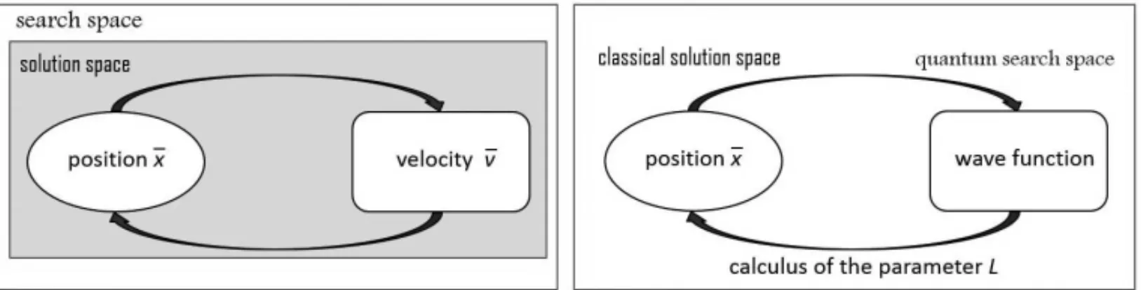
The Quantum PSO (QPSO) algorithm allows the particles to move following the rules defined by the quantum mechanics instead of the classical Newtonian random movement (Sun et al., 2004a, 2004b). In the quantum model of the PSO, the state of each particle is represented by a wave function(x¯,t)instead of the velocity position as it is in the conventional model. The dynamic behavior of the particle is widely divergent of the PSO traditional behavior, where exact values and velocities and positions cannot be determined simultaneously. It is possible to learn the probability of a particle to be in a certain position through the probability of its density function|(x¯,t)|2which depends on the potential field in which the particle is.
In Sun et al. (2004a) and Sung et al. (2004b), the wave function of the particle can be defined by equation (6) where
(x)= √1 L ·e
−p−x
L (6)
and the density of probability is given by the following expression (7).
Q(x)= |(x)|2= 1 L ·e
−2p−x
L (7)
In the quantum inspired PSO model, the search space and the solution space is different in quality. The wave function or the probability function describes the state of the particle in a quantum search space, and it does not provide any information of the position of the particle, what is mandatory to calculate the cost function.
In this context the transformation of a state among these two spaces is essential. Concerning the quantum mechanics, the transformation of a quantum state to a classical state defined in the conventional mechanics is known as collapse. In nature, this is the measure of the position of the particle. The differences between the conventional PSO model and the quantum inspired model are shown in Figure 1 (Sun et al., 2004b).
Figure 1– PSO and QPSO search space.
Due to the quantum nature of the equations, the admeasurements using conventional computers must use the Monte Carlo stochastic simulation method (MMC). The particle position can be defined by equation (8).
x(t)=p±L 2 ln
1 n
. (8)
In Sun et al. (2004a) theL parameter is calculates as in (9) where:
L(t+1)=2·α· p−x(t). (9)
The QPSO interactive equation is defined as
x(t+1)= p±α· p−x(t) ·ln
1 u
, withu=rand(0,1) (10)
In the QPSO algorithm, each particle records itspbestand compares it to all the other particles of the population in order to get thegbestat each iteration. In order to execute the next step, theL parameter is calculated. TheL parameter is considered to be the Creativity or Imagination of the particle, and therefore it is characterized as the scope of search of the knowledge of the particle. The greater the value ofL, the easier the particle acquires new knowledge. In the QPSO the Creativity factor of the particle is calculates as the difference between the current position of the particle and its LIP, as shown in equation (9).
In Shi & Eberhart (1999), the position of the best mean (mbest) is introduced to the PSO, and in Sun et al. (2005a) in the QPSO, thembestis defined as the mean of thepbestof all the particles in the swarm (population), given by expression (11).
mbest= 1 M
M
i=1
pi =
1 M
M
i=1
pi1,
1 M
M
i=1
pi2, . . . ,
1 M
M
i=1
pid
(11)
whereM is the size of the population and piis thepbestofith particle. Thus, equations (9) and
(10) can be redefined as (12) and (13), respectively.
L(t+1)=2·α· mbest−x(t) (12)
x(t+1)=P±α· mbest−x(t) ·ln
1 u
, withu =rand(0,1) (13)
The pseudocode for the QPSO algorithm is described in the following Algorithm 1.
The quantum model of the QPSO shows some advantages in relation to the traditional model. Some peculiarities of the QPSO according to Sun et al. (2004a) can be cited. They are the fol-lowing: quantum systems are complex systems and nonlinear based on the Principle of Superpo-sition of States, in other words, the quantum models have a lot more states than the conventional model; quantum systems are uncertain systems, thus they are very different from the stochastic classical system. Before measurement the particle can be in any state with certain probability and no predetermined final course.
The QPSO algorithm approached up to this point works for continuous problems and not for discrete ones, as the TSP. Some alterations must be implemented in order for this algorithm to be used with discrete problems.
Considerer an initialMpopulation of size four and dimension four represented by the following matrix: M = ⎡ ⎢ ⎢ ⎢ ⎣
1.02 3.56 −0.16 4.5 1.14 −0.10 5.27 1.65 1.63 1.52 0.48 −1.24 1.99 0.97 −1.82 2.24
⎤
⎥ ⎥ ⎥ ⎦
Algorithm 1– QPSO Pseudocode.
Initial Population: Random xi
Do
For i=1until population size M If f(xi) < f(pi)then pi=xi
pg=min(pi)
Calculate mbest using equation (11) For d=1until dimension D
f i1=r and(0,1), f i2=r and(0,1) p= f i1·pid+ f i2·pgd
f i1+ f i2 u=r and(0,1) If r and(0,1) >0.5
xid =p−α· |mbestd−xid| ·ln
1 u
Else
xid =p+α· |mbestd−xid| ·ln
1 u
Until stopping criterion is met
this initial population, one must calculate thepbestof each particle (line) and then verify which is the smallest one. In other words, the particle that shows the smallerpbestalso has the smaller gbest. One must note that depending on the cost function associated to the problem the dimen-sion of the population can be fixed, or, as in the above example, varied. The QPSO can be applied in this case.
Now we have the following context for the TSP. Once matrix M is generated by a uniform distribution, the question is, how can we calculate the objective function associated to the TSP, defined in equation (1), once the cities (vertices of the graph) are numbers that belong to thepos-itive integers?
As a solution we must discretize the continuous values of matrix M in order to calculate the objective or cost function. MatrixM is not modified and its values persist in the execution of the algorithm of the QSPO. The discretization is performed only at the moment the objective function is calculated (Eq. (1)) for a determined solution. Thus, each line of matrixM, a possible solution for problems with four cities, must be discretized.
Pang et al., 2004a; Pang et al., 2004b; Machado & Lopes, 2005; Lopes & Coelho, 2005, but none of them using QPSO.
Thus, for the first line of matrixMwe have:
1.02 3.56 −0.16 4.5 ⇒ 2 3 1 4
where 2 3 1 4
represent a solution for the TSP of four cities. The total discretized matrixMis shown below:
M = ⎡ ⎢ ⎢ ⎢ ⎣
1.02 3.56 −0.16 4.5 1.14 −0.10 5.27 1.65 1.63 1.52 0.48 −1.24 1.99 0.97 −1.82 2.24
⎤
⎥ ⎥ ⎥ ⎦
⇒Mdiscret e= ⎡
⎢ ⎢ ⎢ ⎣
2 3 1 4
2 1 4 3
4 3 2 1
3 2 1 4
⎤
⎥ ⎥ ⎥ ⎦
t our(1) t our(2)
.. .
In this case, there is an evident problem that derives of the use of this simple approach which is clear when there are repeated values in matrixM. In greater problems (many cities) it is possible that some repeated columns may exist in a certain line of matrixM; for example, if the last line of matrixMgiven by [1.99; 1.82; 2.24; 1.99] will be transformed to [2; 1; 4; 3]. In this case, the 1st number 1.99 (1stposition) has priority in relation to the 2ndnumber 1.99 (4thposition) due the minor position in the last line of matrixM.
This fact becomes normal with instances of the TSP with a number of increased cities. The duplicate of the values may not affect the TSP that has an increased number of cities. The dupli-cate of values may not affect the execution of some discrete problems of the CO, however, in the case of the TSP, repeated vertices in the solution are not allowed.
In order to solve this problem the algorithm represented by the pseudocode in the following Algorithm 2 is used.
4 COMPUTATIONAL IMPLEMENTATION AND ANALYSIS OF RESULTS
In this section we present the results from the experiments using the heuristics of LKH enhance-ment and the metaheuristic QPSO previously discussed in section 3 and also a statistics analysis of the same.
The executed algorithms were applied to the instances of the repository TSPLIB. Small, medium and large sized instances were selected to test the optimization approaches selected for the TSP.
For each instance of the problem the algorithm was executed 30 times using different seeds in each of them. The execution form used was the following:
(i) QPSO generates a random initial population;
(iii) QPSO is executed until it finds the best global for the population randomly generated;
(iv) The best global (tour) is recorded in an archive with extension.final;
(v) The LKH is executed using as the initial tour the archive(*.ini)(Rand+LK approach);
(vi) The LKH is executed using as the initial tour the archive(.final)(QPSO+LK Approach);
(vii) The LKH is executed with default parameters (pure LKH).
The size of the populations was fixed in 100 particles and the stop criterion was the optimum value mentioned in the TSPLIB for the approached problem. In the case of the QPSO without LKH, the stopping criterion was a fixed iterations number previously defined as 1000.
In QPSO, Contraction-Expansion Coefficientα is a vital parameter to the convergence of the individual particle in QPSO, and therefore exerts significant influence on convergence of the algorithm. Mathematically, there are many forms of convergence of stochastic process, and dif-ferent forms of convergence have difdif-ferent conditions that the parameter must satisfy. An effi-cient method is linear-decreasing method that decreasing the value ofαlinearly as the algorithm is running. In this paper,αis adopted with value 1.0 at the beginning of the search to 0.5 at the end of the search for all optimization problems (Sun et al., 2005b).
4.1 Results for the Symmetric TSP
Table 1 shows the results for the algorithms: (i) QPSO+LKH, (ii) Rand +LKH, and (iii) LKH, for 10 test problems from the TSPLIB (Reinelt, 1994). The notation “%” was used in this table to represent how much a value for the test problem is distant from the optimum value in percentage.
Note by the results in Table 1 that for the problem swiss42 (Reinelt, 1994), the algorithms QPSO+LKH, Rand+LKH and LKH showed similar performance, including in the statistical analysis by obtaining the best value (optimum value) for the objective function of 1273. Re-garding the problem Gr229, the algorithm Rand+LKH did not achieved the optimum value of 134602, instead, 0.010% of this value. However, the QPSO+LKH and the LKH achieved opti-mum value. The LKH was in mean slightly superior to the QPSO+LKH.
For the problem pbc442 the QPSO+LKH was the fastest algorithm. However the three optimiza-tion approaches achieved optimum value for the objective funcoptimiza-tion which is of 50778. Based on the results of the simulation for the problem Gr666 showed in Table 1 note that the lower stan-dard deviation was achieved by QPSO+LKH but the mean of the results of the objective function for the QPSO+LKH and LKH was identical.
B R UNO M E IRE L L E S H E RRE RA , L E A NDR O C O E L H O a n d M A RIA T E R E S INHA S T E INE R
481
InstanceMethod Minimum (%) Mean (%) Maximum (%) Median (%) Standard deviation
(optimum) time(s)
swiss42 QPSO+LKH 1273 0.000 1273.000 0.000 1273 0.000 1273.0 0.000 0.00 ≈0 (1273) Rand+LKH 1273 0.000 1273.000 0.000 1273 0.000 1273.0 0.000 0.00 ≈0 LKH 1273 0.000 1273.000 0.000 1273 0.000 1273.0 0.000 0.00 ≈0 Gr229 QPSO+LKH 134602 0.000 134615.533 0.010 134616 0.010 134616.0 0.010 2.56 1.8 (134602) Rand+LKH 134616 0.010 134616.000 0.010 134616 0.010 134616.0 0.010 0.00 1.7 LKH 134602 0.000 134613.200 0.008 134616 0.010 134616.0 0.010 5.70 0.1 pcb442 QPSO+LKH 50778 0.000 50778.233 0.000 50785 0.014 50778.0 0.000 1.28 0.3 (50778) Rand+LKH 50778 0.000 50778.233 0.000 50785 0.014 50778.0 0.000 1.28 2.5 LKH 50778 0.000 50778.233 0.000 50785 0.014 50778.0 0.000 1.28 0.8 Gr666 QPSO+LKH 294358 0.000 294444.667 0.029 294476 0.040 294476.0 0.040 52.63 15.9 (294358) Rand+LKH 294358 0.000 294426.833 0.023 294476 0.040 294476.0 0.040 60.76 11.8 LKH 294358 0.000 294426.833 0.023 294476 0.040 294476.0 0.040 60.76 6.6 dsj1000 QPSO+LKH 18660188 0.003 18664570.200 0.026 18681851 0.119 18660188.0 0.003 8944.22 34 (18659688) Rand+LKH 18660188 0.003 18666030.933 0.034 18682099 0.120 18660188.0 0.003 9914.04 25.26
LKH 18660188 0.003 18664537.133 0.026 18681851 0.119 18660188.0 0.003 8961.00 28.16 Pr1002 QPSO+LKH 259045 0.000 259045.000 0.000 259045 0.000 259045.0 0.000 0.00 2.6 (259045) Rand+LKH 259045 0.000 259045.000 0.000 259045 0.000 259045.0 0.000 0.00 1.1 LKH 259045 0.000 259045.000 0.000 259045 0.000 259045.0 0.000 0.00 2.8 pcb1173 QPSO+LKH 56892 0.000 56893.000 0.002 56897 0.009 56892.0 0.000 2.07 8.3 (56892) Rand+LKH 56892 0.000 56892.333 0.001 56897 0.009 56892.0 0.000 1.29 1.3 LKH 56892 0.000 56893.000 0.002 56897 0.009 56892.0 0.000 2.07 9.2 d1291 QPSO+LKH 50801 0.000 50849.750 0.096 50886 0.167 50868.5 0.133 42.07 40.4 (50801) Rand+LKH 50801 0.000 50843.500 0.084 50886 0.167 50843.5 0.084 45.43 40.2 LKH 50801 0.000 50830.100 0.057 50886 0.167 50801.0 0.000 39.60 79.87 u1817 QPSO+LKH 57201 0.000 57242.833 0.073 57313 0.196 57243.0 0.073 37.24 75.5 (50201) Rand+LKH 57225 0.042 57246.250 0.079 57272 0.124 57245.5 0.078 16.06 93.1 LKH 57201 0.000 57237.083 0.063 57272 0.124 57236.5 0.062 17.33 117 Fl3795 QPSO+LKH 28772 0.000 28779.231 0.025 28813 0.143 28772.0 0.000 11.83 1310.3
For the problems d1291 and u1817, the LKH was the method with the best means, remembering that the QPSO+LKH achieved optimum value for at least 30 of the experiments. Note that the Rand+LKH achieved optimum for the d1291, but the best result is 0.042% to reach optimum for problem u1817.
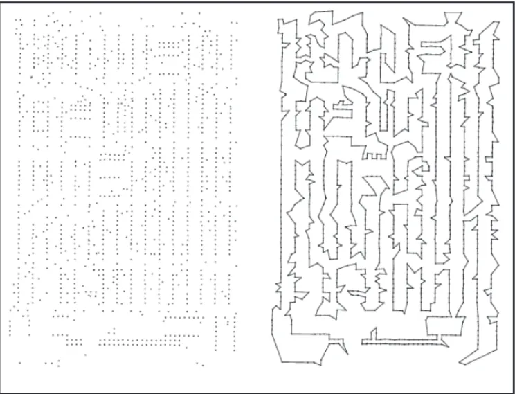
For the large scale symmetric TSP tested in this paper, note that the QPSO+LKH was better and faster than the Rand+LKH and the LKH. Figure 2 shows the best route found for the test problem pcb1173.
Figure 2– Example of the best route found for the problem pcb1173.
4.2 Asymmetric Problems
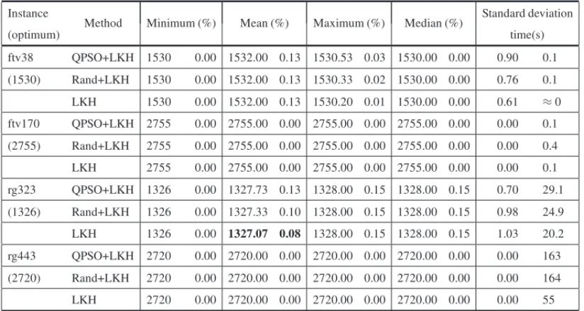
Table 2 shows the results for the algorithms (i) QPSO+LKH, (ii) Rand+LKH and (iii) LKH for the four test problems of the asymmetric TSP of the TSPLIB. As in Table 1, Table 2 used the notation “%” in order to represent how much percent is the achieved value of the test problem distant from the optimum value.
Table 2– Results of optimization of the instances for the asymmetric TSP.
Instance
Method Minimum (%) Mean (%) Maximum (%) Median (%) Standard deviation
(optimum) time(s)
ftv38 QPSO+LKH 1530 0.00 1532.00 0.13 1530.53 0.03 1530.00 0.00 0.90 0.1
(1530) Rand+LKH 1530 0.00 1532.00 0.13 1530.33 0.02 1530.00 0.00 0.76 0.1
LKH 1530 0.00 1532.00 0.13 1530.20 0.01 1530.00 0.00 0.61 ≈0
ftv170 QPSO+LKH 2755 0.00 2755.00 0.00 2755.00 0.00 2755.00 0.00 0.00 0.1
(2755) Rand+LKH 2755 0.00 2755.00 0.00 2755.00 0.00 2755.00 0.00 0.00 0.4
LKH 2755 0.00 2755.00 0.00 2755.00 0.00 2755.00 0.00 0.00 0.1
rg323 QPSO+LKH 1326 0.00 1327.73 0.13 1328.00 0.15 1328.00 0.15 0.70 29.1
(1326) Rand+LKH 1326 0.00 1327.33 0.10 1328.00 0.15 1328.00 0.15 0.98 24.9
LKH 1326 0.00 1327.07 0.08 1328.00 0.15 1328.00 0.15 1.03 20.2
rg443 QPSO+LKH 2720 0.00 2720.00 0.00 2720.00 0.00 2720.00 0.00 0.00 163
(2720) Rand+LKH 2720 0.00 2720.00 0.00 2720.00 0.00 2720.00 0.00 0.00 164
LKH 2720 0.00 2720.00 0.00 2720.00 0.00 2720.00 0.00 0.00 55
5 CONCLUSIONS AND FUTURE WORKS
The troubleshooting of the CO as, for example, the TSP, can be resolved by using recent ap-proaches such as particle swarm concepts and quantum mechanics. The metaheuristic QPSO is an optimization method based on the simulation of the social interaction among individuals in a population. Each element in it moves in a hyperspace, attracted by positions (promising solutions).
The LK heuristic is considered one of the most efficient methods for generating optimum or near-optimum solutions for the symmetric TSP. However, the design and the execution of an algorithm based on this heuristic are not trivial. There are many possibilities for decision making and most of them have a significant influence on the performance (Helsgaun, 2000).
As the Lin-Kernighan heuristic, the QPSO metaheuristic shows many parameters of settings and implementations that directly affects the performance of the proposed algorithm. The algorithm shows promising results for the greater instances(n >1000), range in which the LKH does not produces such efficient results, even though it did not show satisfactory results for small instances of the problem(n <1000)(Nguyen et al., 2007).
REFERENCES
[1] ALBAYRAK M & ALLAHVERDIN. 2011. Development a New Mutation Operator to Solve the Traveling Salesman Problem by Aid of Genetic Algorithms.Expert Systems with Applications,38: 1313–1320.
[2] BAGHERIA, PEYHANIHM & AKBARIM. 2014. Financial Forecasting Using ANFIS Networks with Quantum-behaved Particle Swarm Optimization.Expert Systems with Applications,41: 6235– 6250.
[3] BENIOFFP. 1980. The Computer as a Physical System: a Microscopic Quantum Mechanical Hamil-tonian Model of Computers as Represented by Turing Machines.Journal of Statistical Physics,22: 563–591.
[4] CHENSM & CHIENCY. 2011. Parallelized Genetic Ant Colony Systems for Solving the Traveling Salesman Problem.Expert Systems with Applications,38: 3873–3883.
[5] CHENSM & CHIENCY. 2011. Solving the Traveling Salesman Problem based on the Genetic Sim-ulated Annealing and Colony System with Particle Swarm Optimization Techniques.Expert Systems with Applications,38: 14439–14450.
[6] CHRISTOFIDESN & EILONS. 1972. Algorithms for Large-scale Traveling Salesman Problems. Operational Research,23: 511–518.
[7] CHUANGI & NIELSENM. 2000. Quantum Computation and Quantum Information. Cambridge University Press, Cambridge, England.
[8] COELHOLS & HERRERABM. 2006. Fuzzy Modeling Using Chaotic Particle Swarm Approaches Applied to a Yo-yo Motion System.Proceedings of IEEE International Conference on Fuzzy Systems, Vancouver, BC, Canada, pp. 10508–10513.
[9] COELHOLS. 2008. A Quantum Particle Swarm Optimizer with Chaotic Mutation Operator.Chaos, Solutions and Fractals,37: 1409–1418.
[10] CROES G. 1958. A Method for Solving Traveling Salesman Problems.Operations Research,6: 791–8112.
[11] DONGG, GUOWW & TICKLEK. 2012. Solving the Traveling Salesman Problem using Cooperative Genetic Ant Systems.Expert Systems with Applications,39: 5006–5011.
[12] FANGW, SUNJ, DINGY, WUX & XUW. 2010. A Review of Quantum-behaved Particle Swarm Optimization.IETE Technical Review,27: 336–348.
[13] FEYMANN RP. 1982. Simulating Physics with Computers.International Journal of Theoretical Physics,21: 467–488.
[14] GROVERLK. 1996. A Fast Quantum Mechanical Algorithm for Database Search, Proceedings of the 28th ACM Symposium on Theory of Computing (STOC), Philadelphia, PA, USA, pp. 212–219.
[15] HAMED HNA, KASABOV NK & SHAMSUDDINSM. 2011. Quantum-Inspired Particle Swarm Optimization for Feature Selection and Parameter Optimization in evolving Spiling Networks for Classification Tasks. In: Evolucionary Algorithms (pp. 133–148). Croatia: Intech, 2011.
[17] HERRERA BM & COELHO LS. 2006. Nonlinear Identification of a Yo-yo System Using Fuzzy Model and Fast Particle Swarm Optimization.Applied Soft Computing Technologies: The Challenge of Complexity, A. Abraham, B. de Baets, M. K¨oppen, B. Nickolay (editors), Springer, London, UK, pp. 302–316.
[18] HOFFMANN KL. 2000. Combinatorial Optimization: Current Successes and Directions for the Future.Journal of Computational and Applied Mathematics,124: 341–360.
[19] HOGGT & PORTNOVDS. 2000. Quantum Optimization.Information Sciences,128: 181–197. [20] HOSSEINNEZHADV, RAFIEEM, AHMADIANM & AMELI MT. 2014. Species-based Quantum
Particle Swarm Optimization for Economic Load Dispatch. International Journal of Electrical Power & Energy Systems,63: 311–322.
[21] ISHIBUCHIH & MURATAT. 1998. Multi-objective Genetic Local Search Algorithm and its Ap-plication to Flowshop Scheduling.IEEE Transactions on Systems, Man, and Cybernetics – Part C: Applications and Reviews,28: 392–403.
[22] JASZKIEWICZ A. 2002. Genetic Local Search for Multi-objective Combinatorial Optimization. European Journal of Operational Research,137: 50–71.
[23] JAUY-M, SUK-L, WUC-J & JENGJ-T. 2013. Modified Quantum-behaved Particle Swarm Op-timization for Parameters Estimation of Generalized Nonlinear Multi-regressions Model Based on Choquet integral with Outliers.Applied Mathematics and Computation,221: 282–295.
[24] JOHNSONDS. 1990. Local Optimization and the Traveling Salesman Problem.Lecture Notes in Computer Science,442: 446–461.
[25] JOHNSONDS & MCGEOCHLA. 1997. The Traveling Salesman Problem: A Case Study in Local Optimization in: AARTSEHL & LENSTRAJK (eds.), Local Search in Combinatorial Optimization, John Wiley & Sons, INC, New York, NY, USA.
[26] KENNEDYJ & EBERHARTR. 1995. Particle Swarm Optimization. Proceedings of IEEE Interna-tional Conference on Neural Networks, Perth, Australia, pp. 1942–1948.
[27] LAPORTG. 1992. The Traveling Salesman Problem: An overview of exact and approximate algo-rithms.European Journal of Operational Research,59: 231–247.
[28] LAWLEREL, LENSTRAJK & SHMOYSDB. 1985. The traveling salesman problem: A guided tour of combinatorial optimization. Chichester: Wiley Series in Discrete Mathematics & Optimization.
[29] LI Y, JIAOL, SHANGR & STOLKIN R. 2015. Dynamic-context Cooperative Quantum-behaved Particle Swarm Optimization Based on Multilevel Thresholding Applied to Medical Image Segmen-tation.Information Sciences,294: 408–422.
[30] LINL, GUOF, XIEX & LUOB. 2015. Novel Adaptive Hybrid Rule Network Based on TS Fuzzy Rules Using an Improved Quantum-behaved Particle Swarm Optimization.Neurocomputing, Part B, 149: 1003–1013.
[31] LIN S. 1965. Computer Solutions for the Traveling Salesman Problem. Bell Systems Technology Journal,44: 2245–2269.
[33] LIUF & ZENGG. 2009. Study of Genetic Algorithm with Reinforcement Learning to Solve the TSP. Expert Systems with Applications,36: 6995–7001.
[34] LOPESHS & COELHOLS. 2005. Particle Swarm Optimization with Fast Local Search for the Blind Traveling Salesman Problem.Proceedings of 5th International Conference on Hybrid Intelligent Systems, Rio de Janeiro, RJ, pp. 245–250.
[35] LOURENC¸O HR, PAIXAO˜ JP & PORTUGALR. 2001. Multiobjective Metaheuristics for the Bus-driver Scheduling Problem.Transportation Science,35: 331–343.
[36] MACHADOTR & LOPESHS. 2005. A Hybrid Particle Swarm Optimization Model for the Trav-eling Salesman Problem. H. Ribeiro, R. F. Albrecht, A. Dobnikar, Natural Computing Algorithms, Springer, New York, NY, USA, pp. 255–258.
[37] MANJUA & NIGAMMJ. 2014. Applications of Quantum Inspired Computational Intelligence: a survey,Artificial Intelligence Review,49: 79–156.
[38] MARIANIVC, DUCKARK, GUERRAFA, COELHOLS & RAORV. 2012. A Chaotic Quantum-behaved Particle Swarm Approach Applied to Optimization of Heat Exchangers.Applied Thermal Engineering,42: 119–128.
[39] MERZBACHERE. 1961. Quantum Mechanics.John Wiley & Sons, New York, NY, USA.
[40] MISEVICIUSA, SMOLINSKASJ & TOMKEVICIUSA. 2005. Iterated Tabu Search for the Traveling Salesman Problem: new results.Information Technology and Control,34: 327–337.
[41] MOSHEIOVG. 1994. The Traveling Salesman Problem with Pick-up and Delivery.European Journal of Operational Research,79: 299–310.
[42] NAGATAY & SOLERD. 2012. A New Genetic Algorithm for the Asymmetric Traveling Salesman Problem.Expert Systems with Applications,39: 8947–8953.
[43] NEMHAUSERGL & WOLSEYAL. 1988. Integer and Combinatorial Optimization.John Wiley & Sons, New York, NY, USA.
[44] NETODM. 1999. Efficient Cluster Compensation for Lin-Kernighan Heuristics.PhD Thesis, Depart-ment of Computer Science, University of Toronto, Canada.
[45] NGUYENHD, YOSHIHARAI & YAMAMORIM. 2007. Implementation of an Effective Hybrid GA for Large-Scale Traveling Salesman Problems.IEEE Transactions on System, Man, and Cybernetics-Part B: Cybernetics,37: 92–99.
[46] NGUYENHD, YOSHIHARAI, YAMAMORIK & YASUNAGAM. 2006. Lin-Kernighan Variant. Link: http://public.research.att.com/˜dsj/chtsp/nguyen.txt
[47] PADBERGMW & RINALDIG. 1987. Optimization of a 532-city Symmetric Traveling Salesman Problem by Branch and Cut.Operations Research Letters,6: 1–7.
[48] PANGWJ, WANGKP, ZHOUCG & DONGLJ. 2004a. Fuzzy Discrete Particle Swarm Optimization for Solving Traveling Salesman Problem.Proceedings of 4th International Conference on Computer and Information Technology, Washington, DC, USA, pp. 796–800.
[50] PANGXF. 2005. Quantum Mechanics in Nonlinear Systems.World Scientific Publishing Company, River Edge, NJ, USA.
[51] PAPADIMITRIOUCH & STEIGLITZK. 1982. Combinatorial Optimization – Algorithms and Com-plexity.Dover Publications, New York, NY, SA.
[52] POPPC, KARAI & MARCAH. 2012. New Mathematical Models of the Generalized Vehicle Rout-ing Problem and Extensions.Applied Mathematical Modelling,36: 97–107.
[53] PURISA, BELLOR & HERRERAF. 2010. Analysis of the Efficacy of a Two-Stage Methodology for Ant Colony Optimization: Case of Study with TSP and QAP.Expert Systems with Applications,37: 5443–5453.
[54] REINELTG. 1994. The Traveling Salesman: Computational Solutions for TSP Applications.Lecture Notes in Computer Science, 840.
[55] ROBATIA, BARANIGA, POURHNA, FADAEEMJ & ANARAKIJRP. 2012. Balanced Fuzzy Par-ticle Swarm Optimization.Applied Mathematical Modelling,36: 2169–2177.
[56] RYDNIKV. 1979. ABC’s of Quantum Mechanics.Peace Publishers, Moscow, U.R.S.S.
[57] SAUERJG, COELHOLS, MARIANIVC, MOURELLELM & NEDJAHN. 2008. A Discrete Dif-ferential Evolution Approach with Local Search for Traveling Salesman Problems.Proceedings of the7th IEEE International Conference on Cybernetic Intelligent Systems, London, UK.
[58] SHANKARR. 1994. Principles of Quantum Mechanics, 2nd Edition, Plenum Press.
[59] SHORPW. 1994. Algorithms for Quantum Computation: Discrete Logarithms and Factoring, Pro-ceedings of the35th Annual Symposim Foundations of Computer Science, Santa Fe, USA, pp. 124– 134.
[60] SHI Y, EBERHART R. 1999. Empirical study of particle swarm optimization. Proceedings of Congress on Evolutionary Computation, Washington, DC, USA, pp. 1945–1950.
[61] SILVACA, SOUSAJMC, RUNKLERTA & S ´A DACOSTAJMG. 2009. Distributed Supply Chain Management using Ant Colony Optimization.European Journal of Operational Research,199: 349– 358.
[62] SOSANGM, GALVAO˜ RD & GANDELMANDA. 2007. Algoritmo de Busca Dispersa aplicado ao Problema Cl´assico de Roteamento de Ve´ıculos.Revista Pesquisa Operacional,27(2): 293–310. [63] STEINERMTA, ZAMBONILVS, COSTADMB, CARNIERIC & SILVAAL. 2000. O Problema de
Roteamento no Transporte Escolar.Revista Pesquisa Operacional,20(1): 83–98.
[64] SUNJ, FANGW, WUX, XIEZ & XUW. 2011. QoS Multicast Routing Using a Quantum-behaved Particle Swarm Optimization Algorithm. Engineering Applications of Artificial Intelligence, 24: 123–131.
[65] SUN J, FENG B & XU W. 2004a. Particle Swarm Optimization with Particles Having Quantum Behavior.Proceedings of Congress on Evolutionary Computation, Portland, Oregon, USA, pp. 325– 331.
[67] SUNJ, XUW & FENGB. 2005a. Adaptive Parameter Control for Quantum-behaved Particle Swarm Optimization on Individual Level.Proceedings of IEEE International Conference on Systems, Man and Cybernetics, Big Island, HI, USA, pp. 3049–3054.
[68] SUNJ, XUW & LIUJ. 2005b. Parameter Selection of Quantum-Behaved Particle Swarm Optimiza-tion, International Conference Advances in Natural Computation (ICNC), Changsha, China, Lecture Notes on Computer Science (LNCS) 3612, pp. 543–552.
[69] SUNJ, XUW, PALADEV, FANGW, LAIC-H & XUW. 2012. Convergence Analysis and Improve-ments of Quantum-behaved Particle Swarm Optimization.Information Sciences,193: 81–103. [70] TASGERITEN MF & LIANG YC. 2003. A Binary Particle Swarm Optimization for Lot Sizing
Problem.Journal of Economic and Social Research,5: 1–20.
[71] WANGKP, HUANGL, ZHOUCG, PANGCC & WEI P. 2003. Particle Swarm Optimization for Traveling Salesman Problem.Proceedings of the 2nd International Conference on Machine Learning and Cybernetics, Xi’an, China, pp. 1583–1585.
[72] WANGY, FENGXY, HUANGYX, PUDB, LIANG CY & ZHOUWG. 2007. A novel quantum swarm evolutionary algorithm and its applications.Neurocomputing,70: 633–640.
[73] WILSONEO. 1971. The Insect Societies.Belknap Press of Harvard University Press, Cambridge, MA.