Model of daytime emissions of electronically-vibrationally excited products of O₃ and O₂ photolysis: application to ozone retrieval

www.ann-geophys.net/24/2823/2006/ © European Geosciences Union 2006

Annales

Geophysicae

Model of daytime emissions of electronically-vibrationally excited

products of O

3

and O

2

photolysis: application to ozone retrieval

V. A. Yankovsky and R. O. Manuilova

Institute for Physics of St. Petersburg State University, 1 Ulaynovskaya str., Petergoff, St.-Petersburg, 198504, Russia Received: 2 February 2006 – Revised: 23 August 2006 – Accepted: 6 September 2006 – Published: 21 November 2006

Abstract. The traditional kinetics of electronically excited products of O3 and O2 photolysis is supplemented with

the processes of the energy transfer between electronically-vibrationally excited levels O2(a11g, v) and O2(b16g+, v), excited atomic oxygen O(1D), and the O2 molecules in the

ground electronic state O2(X36−g, v). In contrast to the previous models of kinetics of O2(a11g) and O2 (b16g+), our model takes into consideration the following basic facts: first, photolysis of O3 and O2 and the processes of energy

exchange between the metastable products of photolysis in-volve generation of oxygen molecules on highly excited vi-brational levels in all considered electronic states – b16_g+, a11g and X36−g; second, the absorption of solar radiation not only leads to populating the electronic states on vibra-tional levels with vibravibra-tional quantum number v equal to 0 – O2(b16g+, v=0) (at 762 nm) and O2(a11g, v=0) (at 1.27µm), but also leads to populating the excited electronic– vibrational states O2(b16g+, v=1) and O2(b16g+, v=2) (at 689 nm and 629 nm). The proposed model allows one to calculate not only the vertical profiles of the O2(a11g, v=0) and O2(b16g+, v=0) concentrations, but also the profiles of [O2(a11g, v≤5)], [O2(b16g+, v=1, 2)] and O2(X36g−, v=1– 35). In the altitude range 60–125 km, consideration of the electronic-vibrational kinetics significantly changes the cal-culated concentrations of the metastable oxygen molecules and reduces the discrepancy between the altitude profiles of ozone concentrations retrieved from the 762-nm and

1.27-µm emissions measured simultaneously.

Keywords. Atmospheric composition and structure (Air-glow and aurora; Middle atmosphere – composition and chemistry; Thermosphere – composition and chemistry)

Correspondence to:V. A. Yankovsky ([email protected])

1 Introduction

Measurements of radiation of electronically excited molecu-lar oxygen in the Atmospheric band O2(b16+g, v=0→X36g−, v=0) at 762 nm and in the Infrared Atmospheric band O2(a11g, v=0→X36−g, v=0) at 1.27µm are used for retriev-ing the altitude profile of ozone concentration (e.g. Thomas et al., 1984; Mlynczak et al., 2001). Interpretation of the measurements of emission at 1.27µm is a well known method of determination of the altitude profile of ozone con-centration, and emission at 762 nm was also suggested for this goal in Sica and Lowe (1993a, b). Both methods were realized in Mlynczak et al. (2001). Nowadays, interest in the models of these emissions grows due to the measurements in which both emissions were measured simultaneously in a rocket (Mlynczak et al., 2001) and especially in a satellite experiment (Murtagh et al., 2002).

Metastable molecules and atoms of oxygen are formed in the processes of photodissociation of ozone and oxygen molecules at absorption of ultra-violet radiation of the Sun. These excited products of O3 and O2 photolysis play an

important role in the electronic-vibrational kinetics of O2

molecules and in the heating of the middle atmosphere. The first commonly accepted model of electronic kinetics of these products was developed by Thomas (1984) and Harris and Adams (1983) and was significantly improved by Mlynczak et al. (1993). At present, the model of the electronic kinet-ics of the products of O3 and O2photolysis, developed by

excited electronic state of the O2molecule O2(b16g+)and, further, to the first electronic excited state O2(a11g), play an important role in populating these two electronic states. All these excited states of atomic and molecular oxygen O(1D), O2(b16g+), and O2(a11g)radiate. The corresponding O2

emissions take place in the Atmospheric band:

O2(b16_g+, v=0)→O2(X36_g−, v=0)+hν(λ=762 nm) (1) and in the Infrared (IR) Atmospheric band:

O2(a11g, v=0)→O2(X36g−, v=0)+hν(λ=1.27µm), (2) where v is vibrational quantum number. These emissions are observed using a modern experimental technique. With the use of the kinetic scheme, suggested in Mlynczak et al. (1993), vertical profiles of the ozone abundance are re-trieved from the observations of vertical profiles of these emissions (Mlynczak et al., 2001). At photolysis of ozone in the Hartley band, O2(a11g)is formed with the quantum yield about 90%. It seems evident that the Infrared Atmo-spheric band of O2 at 1.27µm (2), that is formed by

tran-sition from O2(a11g), is preferable for retrieving the pro-files of ozone abundance. This point of view is traditional up to present. However, simultaneously with the production of O2(a11g), the O(1D) atom is formed with the same quantum yield. Therefore, the ozone abundance retrieval could also be carried out using the emission from the state O2(b16g+) at 762 nm (Eq. 1). In the framework of the kinetic model suggested in Mlynczak et al. (1993), it is impossible to de-termine which method of retrieval is more accurate.

Beginning with the publications of the studies of Sparks et al. (1980), Valentini et al. (1987), Thelen et al. (1995), it has been known that the products of O3photolysis must

also be vibrationally excited. Besides that, energy transfer from O(1D) to O2 leads to the formation of

electronically-vibrationally excited molecules O2(b16+g, v) (Streit et al., 1976; Lee and Slanger, 1978). Mlynczak et al. (1993) sup-posed that vibrational kinetics can be neglected, which is possible only if the processes of vibrational-vibrational (V-V) and vibrational-translational (V-T) energy transfer be-tween vibrational sublevels of electronic states are much faster than collisional deactivation of electronically excited states. However, the present laboratory and theoretical data on the kinetics of the excited products of ozone and oxy-gen photolysis (Hwang et al., 1999; Slanger and Copeland, 2003; Dylewski et al., 2001; Kalogerakis et al., 2002; Pe-jakovic et al., 2005) have given new information about the processes of energy exchange between electronic-vibrational levels, which are fast enough to compete with the processes of V-V and V-T energy exchange. These works made it nec-essary to create a model of electronic-vibrational kinetics of the excited products of O3 and O2 photolysis because the

fast processes of energy exchange between electronically-vibrationally excited levels could not be considered in the framework of only electronic kinetics. It should also be

noted, that transitions O2(b16g+, v→X36g−, v′′) have also been observed in atmospheric experiments. Skinner and Hays (1985), analyzing the brightness of the Atmospheric band of O2 in the daytime thermosphere measured by the

Dynamic Explorer 2 in the altitude interval 60–300 km, took into account the contributions of transitions O2(b16g+, v→X36_g−, v′′) for bands (0-0), (1-1), (2-2). We will show in this study that the traditional kinetics of electronically excited products of O3 and O2 photolysis should be

sup-plemented with the processes of energy transfer between electronically-vibrationally excited levels O2(a11g, v) and O2(b16g+, v), excited atomic oxygen O(1D) and the O2

molecules in the ground electronic state O2(X36g−, v). In contrast to the previous models of kinetics of O2(a11g)and O2(b16+g), our model takes into consideration the following basic facts: first, photolysis of O3and O2and the processes

of energy exchange between the metastable products of pho-tolysis involve generation of oxygen molecules on highly ex-cited vibrational levels in all considered electronic states – b16+

g, a11gand X36g−; second, the absorption of solar ra-diation not only leads to populating the electronic states on vibrational levels with vibrational quantum number v equal to 0 – O2(b16+g, v=0) (at 762 nm) and O2(a11g, v=0) (at 1.27µm), but also leads to populating the excited electronic– vibrational states O2(b16g+, v=1) and O2(b16g+, v=2) (at the 689 nm and 629 nm). In the framework of this study we will compare the models of pure electronic and electronic-vibrational kinetics and show the difference between the two models for the direct problem of calculations of the volume emission rates of the 762-nm and 1.27-µm bands and for the inverse problem of ozone retrieval from both emissions. As it will be shown below, considering the electronic-vibrational kinetics significantly changes the calculated concentrations of the metastable oxygen molecules above 60 km and reduces the discrepancy between the altitude profiles of ozone con-centrations retrieved from the 762-nm and 1.27-µm emis-sions measured simultaneously.

2 Kinetics of electronically-vibrationally excited prod-ucts of O3and O2photodissociation in the middle

at-mosphere

In Fig. 1, the scheme of electronic-vibrational kinetics of the products of O3 and O2 photolysis is presented. The

excited electronic states are shown by bold lines, and the vibrational levels of these electronic states are shown by thin lines. The vibrational number is denoted by the letter v. The circles with italic letters in Fig. 1 denote all types of processes that were taken into account. References to the values of the rates of photodissociation of O2 and

O3 and of photoexcitation of O2 used in this study are

a

35 34 V

V 33

2

4 1

0 3

2 1 0

4 3 2 1

k(X,v→v-2; N2) k(b,v; M)

O2(b1Σ+g, v)

e

JHu, JCh

k(X,v; M)

gIRA

O2(X3Σ-g, v)

k(a,v; M) JSRC

JLy α O(1D)

JH

gA

gB

gγ 630 nm

1270 nm 762 nm

d

g

O2 O3

c

JH

h

f

b

O2(a1Δg,v)

j

l

k

i

O(3P) O2(X3Σ-g)

Fig. 1.The scheme of electronic-vibrational kinetics of the products of O3and O2photolysis in the middle atmosphere.

Table 1.Processes of O2and O3photodissociation and photoexcitation. Short notations for electronically excited states of oxygen molecule

in Tables 1–5: O2(b16+g, v)=O2(b, v), O2(a11g, v)=O2(a, v), O2(X36g−, v)=O2(X, v). J – rate of photodissociation and photoexcitation at

the top of the atmosphere, F – quantum yield of the products.

Reaction J (s−1) F Ref.

O2+hν(SRC)→O(3P)+O(1D) 2.60×10−6 1.0 Rodrigo et al. (1986), DeMore et

al. (1997)

O2+hν(Lyman-α)→O(3P)+O(1D) 3.40×10−9 0.48–0.58 Rodrigo et al. (1986), Reddmann and

Uhl (2003)

O3+hν→O2(X, v=0–35)+O(3P)

O3+hν→O2(a, 5)+O(1D)

O3+hν→O2(a, 4)+O(1D)

O3+hν→O2(a, 3)+O(1D)

O₃+hν→O₂(a, 2)+O(1D) O3+hν→O2(a, 1)+O(1D)

O₃+hν→O₂(a, 0)+O(1D)

8.00×10−3

0.10∗ 0.045∗ 0.072∗ 0.072∗ 0.135∗ 0.135∗ 0.441∗

Svanberg et al. (1995) Michelson et al. (1994), Sparks et al. (1980), Thelen et al. (1995), Valentini et al. (1987), Ball et al. (1995), Klais et al. (1980), DeMore et al. (1997), Dylewski et al. (2001)

O2+hν(762 nm band)→O2(b, 0) 5.35×10−9 Bucholtz et al. (1986), Mlynczak et al.

(1996) O2+hν(689 nm band)→O2(b, 1) 2.94×10−10

O2+hν(629 nm band)→O2(b, 2) 7.94×10−12

O2+hν(1.27µm)→O2(a, 0) 1.54×10−10

* – Presented values are quantum yields forλ=254 nm, however, all calculations of the rate of O3photodissociation in the Hartley band are

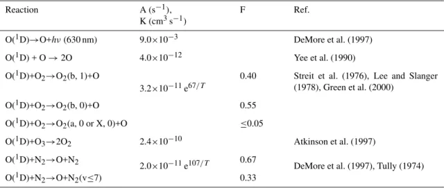
Table 2.Processes of O(1D) deactivation. A – Einstein coefficient, K – rate constant of reaction, other symbols as in Table 1.

Reaction A (s−1),

K (cm3s−1)

F Ref.

O(1D)→O+hν(630 nm) 9.0×10−3 DeMore et al. (1997)

O(1D) + O→2O 4.0×10−12 Yee et al. (1990)

O(1D)+O2→O2(b, 1)+O

3.2×10−11e67/T

0.40 Streit et al. (1976), Lee and Slanger

(1978), Green et al. (2000)

O(1D)+O2→O2(b, 0)+O 0.55

O(1D)+O2→O2(a, 0 or X, 0)+O ≤0.05

O(1D)+O3→2O2 2.4×10−10 Atkinson et al. (1997)

O(1D)+N2→O+N2

2.0×10−11e107/T 0.67 DeMore et al. (1997), Tully (1974)

O(1D)+N2→O+N2(v≤7) 0.33

a – photolysis of O2 in the Schumann-Runge

contin-uum (SRC) in the 120–174-nm region and in the Lyman-α

line (Table 1):

O2+hν (SRC,Lyman−α)→O(1D)+O(3P); (3)

these processes are the main sources of O(1D) atoms above 80 km (e.g. Rodrigo et al., 1986);

b – photolysis of O3 in the singlet channel (the Hartley

band at 200–310 nm) (Table 1):

O3+hν(the Hartley band)→O2(a11g, v=0−5)+O(1D);(4)

c – EE′ transfer of electronic excitation energy from the O(1D) atom to the oxygen molecule. The process of energy transfer from O(1D) excites not only vibrational level 0, but also vibrational level 1 of the electronic state O2(b16g+) (Ta-ble 2):

O(1D)+O2(X36−g, v=0)→O2(b16+g, v≤1)+O( 3

P);(5)

d– excitation of all three considered vibrational levels of the electronic state O2(b16g+)due to direct absorption of solar radiation. The rates of absorption at 762, 689 and 629 nm were taken from Bucholtz et al. (1986); Mlynczak and Mar-shall (1996) (Table 1):

O2+hν(762; 689; 629 nm) →O2(b16+g, v=0,1,2), (6) respectively;

e– quenching of vibrational excitation of O2(b16g+, v≥1) due to intramolecular near resonance electronic-electronic (EE) exchange (Table 3):

O2(b16_g+, v≤2)+O2(X36_g−, v=0)

→O2(X36_g−, v≤2)+O2(b16_g+, v=0); (7)

a specific feature of this type of reaction is that the electronic level changes in the initially excited oxygen molecule, while the vibrational quantum number v remains unchanged, and electronic excitation transfers to the collisional partner. Such reactions are from 2 to 3 orders of magnitude faster than the reactions of intermolecular energy transfer between electronic levels (reactions of the typefin Fig. 1);

f – formation of O2(a11g, v=0–3) at collisional quenching of O2(b16g+, v=0) by the electronic-vibrational (EV) type of the energy exchange (Table 2):

O2(b16g+, v=0)+M(=O2, N2, O(3P),O3,CO2)

→O2(a11g, v≤3)+M; (8)

g– the process of excitation of O2(a11g, v=0) due to direct absorption of solar radiation (Table 1):

O2+hν(1.27µm)→O2(a11g, v=0); (9)

h– the process of EE quenching of O2(a11g, v), similar to the channele(Table 4):

O2(a11g, v)+O2(X36g−,v=0)

→O2(X36_g−, v)+O2(a11g,v=0); (10)

i– quenching of O2(a11g, v=0) of the type similar to EV-exchange (Table 4):

O2(a11g,v=0)+O2(X36g−,v=0)

→O2(X36g−, v≤5)+O2(X36g−, v′′=5−v); (11)

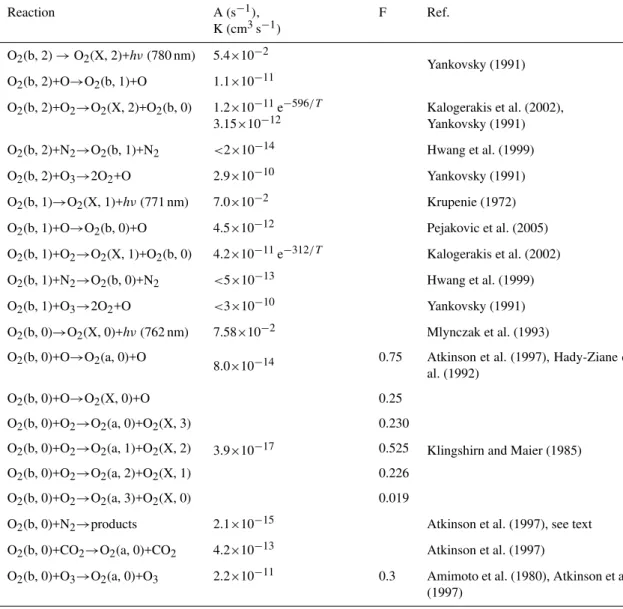
Table 3.Processes of deactivation of O2(b16g+, v). Symbols as in Tables 1 and 2.

Reaction A (s−1),

K (cm3s−1)

F Ref.

O2(b, 2)→O2(X, 2)+hν(780 nm) 5.4×10−2

Yankovsky (1991) O2(b, 2)+O→O2(b, 1)+O 1.1×10−11

O2(b, 2)+O2→O2(X, 2)+O2(b, 0) 1.2×10−11e−596/T

3.15×10−12

Kalogerakis et al. (2002), Yankovsky (1991)

O2(b, 2)+N2→O2(b, 1)+N2 <2×10−14 Hwang et al. (1999)

O2(b, 2)+O3→2O2+O 2.9×10−10 Yankovsky (1991)

O2(b, 1)→O2(X, 1)+hν(771 nm) 7.0×10−2 Krupenie (1972)

O2(b, 1)+O→O2(b, 0)+O 4.5×10−12 Pejakovic et al. (2005)

O2(b, 1)+O2→O2(X, 1)+O2(b, 0) 4.2×10−11e−312/T Kalogerakis et al. (2002)

O2(b, 1)+N2→O2(b, 0)+N2 <5×10−13 Hwang et al. (1999)

O2(b, 1)+O3→2O2+O <3×10−10 Yankovsky (1991)

O2(b, 0)→O2(X, 0)+hν(762 nm) 7.58×10−2 Mlynczak et al. (1993)

O2(b, 0)+O→O2(a, 0)+O

8.0×10−14 0.75 Atkinson et al. (1997), Hady-Ziane et

al. (1992)

O2(b, 0)+O→O2(X, 0)+O 0.25

O₂(b, 0)+O₂→O₂(a, 0)+O₂(X, 3)

3.9×10−17

0.230

Klingshirn and Maier (1985)

O₂(b, 0)+O₂→O₂(a, 1)+O₂(X, 2) 0.525

O₂(b, 0)+O₂→O₂(a, 2)+O₂(X, 1) 0.226

O₂(b, 0)+O₂→O₂(a, 3)+O₂(X, 0) 0.019

O₂(b, 0)+N₂→products 2.1×10−15 Atkinson et al. (1997), see text

O₂(b, 0)+CO₂→O₂(a, 0)+CO₂ 4.2×10−13 Atkinson et al. (1997)

O₂(b, 0)+O₃→O₂(a, 0)+O₃ 2.2×10−11 0.3 Amimoto et al. (1980), Atkinson et al.

(1997)

k – the processes of vibrational-vibrational (V-V) and vibrational-translational (V-T) deexcitation of vibrational levels O2(X36−g, v) for v=1–35 (Table 5):

O2(X36g−, v≤35)+O2(X36−g, v=0)

→O2(X36g−, v−1)+O2(X36g−, v=1), (13) O2(X36g−, v≤35)+M(=O2, N2, O(3P), O3)

→O2(X36_g−, v−1)+M; (14)

l– the process of VV two-quantum transition in collisions of O2(X36g, v) with N2for v=12–26 (Table 5):

O2(X36_g−,12≤v≤26)+N2(X16, v=0)

→O2(X36_g−, v−2)+N2(X16, v=1). (15)

The vibrational levels of the ground electronic state are pop-ulated by the processes of electronic-vibrational (EV) energy exchange with the state O2(a11g, v=0) (Eq. 11). As it was noted above, at ozone photolysis in the Hartley, Huggins and Chappius bands, the vibrational levels of the ground elec-tronic level O2(X36g−, v) are excited up to the value of v=35 (Eq. 12). Other processes which populate vibrational lev-els are the processes of EE exchange with the corresponding levels of the electronic states O2(b16g+, v) for v=0–2 (Eq. 6) and O2(a11g, v) for v=1–5 (Eq. 10).

In Table 1 the rates of photodissociation of O2and O3and

of photoexcitation of O2(b16g+, v) and O2(a11g, v=0) used in this study are presented. The quantum yield of O(1D) for-mation in the O2photolysis in the Schumann-Runge

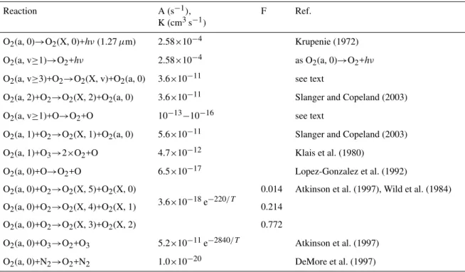
Table 4.Processes of deactivation of O2(a11g, v). Symbols as in Tables 1 and 2.

Reaction A (s−1),

K (cm3s−1)

F Ref.

O₂(a, 0)→O₂(X, 0)+hν(1.27µm) 2.58×10−4 Krupenie (1972)

O2(a, v≥1)→O2+hν 2.58×10−4 as O2(a, 0)→O2+hν

O2(a, v≥3)+O2→O2(X, v)+O2(a, 0) 3.6×10−11 see text

O2(a, 2)+O2→O2(X, 2)+O2(a, 0) 3.6×10−11 Slanger and Copeland (2003)

O2(a, v≥1)+O→O2+O 10−13−10−16 see text

O2(a, 1)+O2→O2(X, 1)+O2(a, 0) 5.6×10−11 Slanger and Copeland (2003)

O2(a, 1)+O3→2×O2+O 4.7×10−12 Klais et al. (1980)

O2(a, 0)+O→O2+O 6.5×10−17 Lopez-Gonzalez et al. (1992)

O2(a, 0)+O2→O2(X, 5)+O2(X, 0)

3.6×10−18e−220/T

0.014 Atkinson et al. (1997), Wild et al. (1984)

O2(a, 0)+O2→O2(X, 4)+O2(X, 1) 0.214

O2(a, 0)+O2→O2(X, 3)+O2(X, 2) 0.772

O2(a, 0)+O3→O2+O3 5.2×10−11e−2840/T Atkinson et al. (1997)

O2(a, 0)+N2→O2+N2 1.0×10−20 DeMore et al. (1997)

Table 5.Processes of energy transfer and deactivation of O2(X36g−, v). Symbols as in Tables 1 and 2.

Reaction K (cm3s−1) F Ref.

O3+O→O2(X, v=0–30)+O2 5.6×10−12e−1959/T F(v) Balakrishnan and Billing

(1996)

O2(X, v≥5)+O→O2+O KV T=5×10−11×(T/300)0.5 Breig (1969), Webster and

Bair (1972)

O2(X, v=2–4)+O→O2+O KV T(v)∗=1.1×10−12×(T/300) e1.0·v

O2(X, v=1)+O→O2+O KV T=3×10−12 Slanger and Copeland

(2003)

O2(X, v)+O2→O2(X, v–1)+O2(X, v=1) KV V(v=2)=2.0×10−13

KV V(v=3)=2.6×10−13

Kalogerakis et al. (2005)

O2(X, v=4–20)+O2→O2(X, v-1)+O2(X, 1) KV V(v)∗=1.3×10−12e−0.31·v Slanger (1997), Coletti and

Billing (2002)

O2(X, v>20)+O2→O2(X, v–1)+O2 KV T(v)∗=6×10−17×(T/300) e0,2·v

O₂(X, v=12–17)+N₂→O₂(X, v–2)+N₂(X, v=1) K_{V V}′(v)∗=3.6×10−19e0,66·v

Slanger (1997) O₂(X, v=18–26)+N₂→O₂(X, v–2)+N₂(X, v=1) K_{V V}′(v)∗=4.5×10−13e−0,173·v

O₂(X, v=1)+O₂→2O₂ K_{V T}=4.2×10−19×(T/300)0,5

Lopez-Puertas et al. (1995) O₂(X, v=1)+N₂→O₂+N₂(X, v=1) K_{V V}′(v)=4.2×10−19×(T/300)0,5

the Hartley bands, the spectral dependence of quantum yield of O(1D) and, correspondingly, of O2(a11g), is known in detail (Michelsen et al., 1994). For O2(a11g, v), the quan-tum yields significantly depend on wave length (Sparks et al., 1980; Valentini et al., 1987; Thelen et al., 1995). The quan-tum yields of O2(a11g, v) were measured for 6 wavelengths for v=0–7 from 235 to 285 nm (Dylewski et al., 2001). These data show that the part of the electronically-vibrationally excited molecules produced at O3photolysis changes from

30% at 285 nm to 70% at 235 nm. At the Hartley band max-imum in the region of 254 nm this part is about 60%. This is why for O2(a11g, v) the quantum yields should be known at all wavelengths. With the purpose of presenting the quan-tum yield as a function of wavelength, we constructed in-terpolated formulas for quantum yield dependence on the wave numbers in the whole interval of the Hartley band 200– 320 nm, for all vibrational quantum numbers from 0 to 5 (Yankovsky and Kuleshova, 2006), using all published ex-perimental data. In particular, it enables us to calculate the total production rate of O2(a11g, v) in O3photodissociation

in the Hartley band by integration of these functions, the rates of photodissociation and the cross sections of solar radiation absorption over the wavelength. The vibrational levels with v equal to 6 and 7 are excited by radiation, with the wave-length shorter than 240 nm, for which the cross section of O2absorption is small and the processes of excitation of the

levels with v=6, 7 can be neglected.

The triplet channel of O3 photodissociation in the

Hart-ley band gives the formation of O2(X36−g, v=0–35). The quantum yields of O2(X36g−, v) also depend significantly on the wavelength. We used the calculations of the quantum yields of O2(X36g−, v) in the Hartley band from Svanberg et al. (1995). At O3photodissociation in the Chappius and

Huggins bands the levels O2(X36−g, v) are formed at v=0– 15. The cross section of the absorption of solar radiation in the Chappius and Huggins bands is small, so the O3

pho-todissociation in the Chappius and Huggins bands does not influence the production of O2(X36−g, v) significantly.

In Table 2, the Einstein coefficient for emission of O(1D) at 630 nm and the rate constants of O(1D) deex-citation at collisional processes, as well as the quantum yields of electronically-vibrationally excited products of these processes, are presented. In Green et al. (2000) the total quantum yield of O2(b16g+, v≥0) in the reaction O(1D)+O2→O2(b16g+, v≥0)+O was estimated to be equal to 0.95. In correspondence with the value of the total quan-tum yield we calculated the quanquan-tum yields of O2(b16g+, v=1) and O2(b16g+, v=0), based on the results of Lee and Slanger (1978).

In Table 3, the Einstein coefficients for emissions of O2(b16g+, v) at 780, 771, and 762 nm and the rate constants of deexcitation of O2(b16g+, v) at collisional processes, as well as the quantum yields of O2(a11g, v) and O2(X36g−, v) for v from 0 to 3 formed in these processes, are presented.

The rate constant of the reaction O2(b16g+, v=2)+O2(X36g−, v=0)→O2(X36g−, v=2)+O2(b16g+, v=0) was measured in the experiment of Kalogerakis et al. (2002) in the temper-ature range 110–298 K and in the experiment of Yankovsky (1991) in the range 340–445 K. Both sets of the data corre-spond to each other. In our calculations we used our approx-imation of the data of Kalogerakis et al. (2002).

For processes of deexcitation of the states O2(b16g+, v=1, 2) by N2only the upper limit of the values of the rate

con-stants are known. Our estimations show that these reac-tions don’t influence the populareac-tions of the states O2(b16g+, v=1, 2). In Tables 3 and 4 the processes of quenching the states O2(b16g+, v) and O2(a11g, v) at collisions with O3are

shown in connection with high values of the rate constants of these processes. However, in the mesosphere the role of such processes is insignificant because of low abundance of ozone. We should discuss the influence of the possible values of quantum yields of the products of the reaction of quench-ing of O2(b16g+, v=0) by N2. In the model of Mlynczak et

al. (1993) it is supposed that the quantum yield F(a, 0) of the process

O2(b16g+,v=0)+N2

→O2(a11g,v=0)+N2(X, v=2)+607.1 cm−1 (16) is equal to 1. However, the rate constant of the reaction of quenching of O2(b16g+, v=0) by N2 is almost 100 times

greater than the rate constant of the reaction of quenching O2(b16g+, v=0) by O2. In the framework of

electronic-vibrational kinetics, possible pathways of the process of quenching of O2(b16+g, v=0) by N2should be considered.

The relatively high value of the rate constant for quenching by N2, led Braithwaite et al. (1976) to the suggestion that the

following quasi-resonance process might exist: O2(b16_g+,v=0)+N2

→O2(a11g,v=2)+N2(X, v=1)−31.9 cm−1. (17) However, another quasi-resonance process is also possible: O2(b16g+, v=0)+N2

→O2(X36g−, v=9)+N2(X, v=0)−52.8 cm−1. (18)

There is no information about possible values of the quan-tum yields of the products of this reaction; however, the ratio between the two pathways of the reaction influence distinctly the ozone concentration retrieval at the region of the second ozone maximum. This is why we consider the suggestion that both quasi-resonance processes (Eqs. 17, 18) exist and are assumed to have the same values of the quantum yields O2(a11g, v=2), F(a, 2), and O2(X36−g, v=9), F(X, 9). For our calculations we used F(a, 2) and F(X, 9) equal to 0.5.

was taken from Krupenie (1972). For the Einstein coeffi-cients for emissions of O2(a11g, v=1–5) the same value was used, because the experimental data are absent. However, ra-diative deexcitation of O2(a11g, v≥1) can be neglected in the calculations of O2 (a11g, v) concentration, due to the fact that the rate of radiative deexcitation is much smaller than the rates of deexcitation at collisions with O2 (Slanger

and Copeland, 2003).

The rate constants of deexcitation of O2(a11g, v≥3) in collisions with O2 have not been measured and for these

processes we used the value of the rate constant of the process O2(a11g, v=2)+O2 that was measured by Slanger

and Copeland (2003). For the processes of collisions of O2(a11g, v≥1) with atomic oxygen the rate constants have not been measured either. So we varied the values of the rate constants of these processes from 10−13 _{to 10}−16_cm3_s−1_.

Even for such a broad range of the values of the rate con-stants these processes do not affect the results of the calcula-tions of O2(a11g, v=0) concentration. In Table 4 the quan-tum yields of O2(X36g−, v=0–5) in the reaction of collisions of O2(a11g, v=0) with O2(Wild et al., 1984) are presented.

The values of the rate constants of the reactions of deex-citation of electronically-vibrationally excited O2molecules

O2(a11g, v≥1) at collisions with N2 are so small that

such processes do not affect the populations of electronic-vibrational levels under consideration in comparison with the processes of deexcitation at collisions with molecular oxy-gen. For estimations we used the maximum value for these rate constants 8.4×10−14cm3s−1 from Klais et al. (1980), which is two orders of magnitude smaller than the rate con-stants of the processes of deexcitation at collisions with molecular oxygen.

The role of quenching electronically excited molecules O2(a11g, v=0) by N2is significant, and the corresponding

process was taken into account (see Table 4).

In Table 5 the rate constants of V-V and V-T processes of O2(X36−g, v) collisional excitation and deexcitation are pre-sented. In order to calculate the populations of vibrational levels for v=1–35, approximations of the dependencies of rate constants on vibrational quantum numbers on the basis of the known experimental data must be carried out. The pre-sented approximations (see Table 5) give a convenient form for the calculations of the values of the rate constants used in our model within the limits of experimental data errors. With the purpose of constructing kinetic equations for v≤35, the rate constants of V-T deexcitation of O2(X36g−, v) in colli-sions with O2calculated for v≤30 (Coletti and Billing, 2002)

were extrapolated for v≤35.

The ozone and oxygen photodissociation is a non-equilibrium stationary process. For a description of such kind of processes, using the principle of detailed equilibrium is inapplicable for the calculation of the rate constant of the inverse process of the upper state excitation by the transition from the lower state. This is why we don’t use the

princi-ple of detailed equilibrium for calculations of populations of the considered electronic-vibrational states. For inverse pro-cesses of V-V and V-T energy transfer between vibrational states of the ground electronic state O2(X36g−, v), we use the rate constants calculated by Billing et al. (1992); Coletti and Billing (2002) from the measured cross sections of col-lisional reactions. The inverse processes of populating the electronically-vibrationally excited states O2(b16g+, v) and O2(a11g, v) are insignificant in comparison with the pro-cesses of populating from the upper states or directly by pho-todissociation, because the energy difference is greater than 1 eV. The estimations show that in our model we can neglect these processes.

The experimental methods of the measurements of the rate constants of deexcitation processes could be conventionally divided into two groups: measurements for low (200–400 K) and those for high temperatures, for example, experiments in shock tubes, which were carried out at the temperatures of higher than one thousand Kelvins. It should be noted that at high temperatures the measured rate constant might be a superposition of the rate constants for several states (Polack, 1979). In accordance with the atmospheric conditions, we use the values of the rate constants measured in the tempera-ture interval 150–350 K.

At conditions when the local thermodynamic equilibrium (LTE) for electronic-vibrational states does not exist, the populations of the states are calculated by solving the system of kinetic equations for all 45 electronic-vibrational states under consideration: the first excited state of atomic oxygen, O(1_{D), three states of O}

2(b16+g, v), six states of O2(a11g, v) and 35 states of O2(X36g−, v).

The populations of the states of these excited species are described by the system of differential equations:

∂ni

∂t = X

k6=i

(nk·pi,k)−ni·qi +Fi, (19) wherei– the state number (i=1–45),ni – the population of the i-th state, pi,k – the production rate of species i from speciesk (k=1–45, k6=i)in collisional processes of energy transfer,qi – the total loss rate of speciesiin the processes of collisional and radiative deactivation,Fi– the volume pro-duction rate of thei-th species in the processes of photolysis of O2 and O3molecules and in chemical reactions (for

ex-ample, in the reaction of collision of O with O3).

Then the system of differential Eqs. (19) can be presented as a matrix equation for the vector of the state populationsn

∂n

∂t =A·n+F. (20)

We are solving a stationary problem. In this case the system of equations is written as a linear algebraic system

n_=A−1_{·F. (21)}

Olemskoy (2006). In order to derive the ozone concentra-tion from the measured intensities of emissions, the system of implicit algebraic equations is solved by the method of parameter fitting.

The computer code for calculating the rate of photodisso-ciation of ozone and molecular oxygen, taking into account the spectral dependence of quantum yields of the products of O2and O3photolysis in the interval of wavelengths from 120

to 850 nm, was developed. The computer code enables us to calculate the rates of: 1) the formation of O(1D) atoms in the O2photolysis in the Schumann-Runge continuum and in

the Lyman-αline (3) and O3photolysis in the Hartley band

(4); 2) the formation of O2(a11g,v) in O3 photolysis in the

Hartley band (4); 3) the formation of O2(X36g−, v) in O3

photolysis in the Hartley, Chappius and Huggins bands (12) for different solar zenith angles (from−80◦to 80◦SZA). In our calculations of the photodissociation rate, the model of photodissociation in the Schumann-Runge continuum, sug-gested by DeMajistre et al. (2001), and the model of pho-todissociation in the Schumann-Runge bands, suggested by Koppers and Murtagh (1996), were used. In the code model MSIS 90 was used for the main atmospheric constituents, the O3 model was taken from Keating et al. (1989), the

atomic oxygen model was taken from Llewellyn and Mc-Dade (1996), the CO2model was taken from Kauffmann et

al. (2002). The solar spectrum was taken from Allen and Frederick (1982). The photodissociation cross sections of the solar radiation for the Hartley bands were taken from De-More et al. (1997).

In this way, the developed method enables us to calculate the altitude profiles of the concentration of O2molecules in

any considered electronic-vibrational state in the middle at-mosphere. However, at present, only the information about the populations of O2(a11g, v=0) and O2(b16g+, v=0) can be obtained from the atmospheric experiments. In principle, the formulation and solution of the inverse problem for any state under consideration is possible, but the accuracy of the solu-tion for upper states decreases because the values of the rate constants are less known and the populations of these states are much smaller than for the lower states.

3 Concentrations of electronically-vibrationally excited oxygen in the middle atmosphere

The proposed model was used to calculate the altitude pro-files of the number densities of O2molecules in

electronic-vibrational states. The calculations were made for the condi-tions of the experiment METEORS (Mlynczak et al., 2001), in which both emissions at 762 nm and 1.27µm were mea-sured simultaneously. It was carried out for 32◦_{N and for the} Solar zenith angle 38◦_.

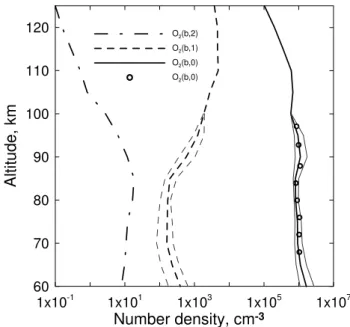
In Fig. 2 the altitude profiles of the number densities of the molecules in the states O2(b16g+, v) for v=0, 1 and 2 and the measured number densities of O2(b16g+, v=0) (Mlynczak et

1x10-1 1x101 1x103 1x105 1x107

Number density, cm-3

60 70 80 90 100 110 120

A

lt

it

ude, km

O2(b,2)

O2(b,1)

O2(b,0)

O2(b,0)

Fig. 2.Altitude profiles of the number densities of the molecules in the state O2(b16g+, v) for v=0, 1 and 2. Circles – experimental data

of METEORS for O2(b16g+, v=0) (Mlynczak et al., 2001). The

bold curves – calculations for the conditions of experiment METE-ORS in accordance with our model. The altitude profiles of the number densities of molecules in the states O2(b16g+, v) for v=0

and 1, calculated for two ozone altitude profiles [O3]′at variations

of [O₃]′/[O₃] equal to 0.5 and 2.0, are shown by thin grey lines.

al., 2001) are shown. With the purpose of showing how the choice of the [O3] profile other than the one from Keating

et al. (1989) changes the results, the altitude profiles of the number densities of molecules in the states O2(b16g+, v) for v=0 and 1 were also calculated for two other ozone altitude profiles [O3]′, for variations of [O3]′/[O3] equal to 0.5 and

2.0.

0 20 40 60 80 100 Contribution, %

60 70 80 90 100 110 120

Altitude, km

1

2

3

4

5

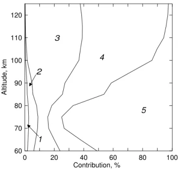
Fig. 3.Areas of diagram indicate the relative contributions of direct and indirect processes to the total rate of O2(b16+g, v=0)

produc-tion, in percent. Indirect processes: 1 – absorption of solar radi-ation O2+hν (629 nm)→O2(b16g+, v=2) (magnified by 10); 2 –

absorption of solar radiation O2+hν(689 nm)→O2(b16g+, v=1); 3

– energy transfer O(1D)→O2(b16g+, v=1). Direct processes: 4 –

energy transfer O(1D)→O2(b16g+, v=0); 5 – absorption of solar

radiation O₂+hν(762 nm)→O₂(b16_g+, v=0).

v=0)→O2(X36g−, v=1)+O2(b16+g, v=0). The minimum of the contributions of channels 3 and 4 in Fig. 3 at 70–80 km is connected to the fact that below 80 km the channel of the O(1D) formation in the O2photolysis in the

Schumann-Runge continuum (Eq. 3), dominating at higher altitudes, gives way to the formation of O(1D) in ozone photolysis in the Hartley band (4).

In Fig. 4 the altitude profiles of the number densities of the molecules in the states O2(a11g, v) for v=0, 1, 2 and 4 and the measured number densities of O2(a11g, v=0) (Mlynczak et al., 2001) are shown, although the calculations were also made for v=3 and 5. With the purpose of showing how the choice of the [O3] profile other than the one from Keating

et al. (1989) changes the results, the altitude profiles of the number densities of the molecules in the states O2(a11g, v) for v=0 and 1 were also calculated for two variations of [O3]′/[O3], equal to 0.5 and 2.0.

In Fig. 5 the relative contributions of the different pro-cesses to the total rate of production of O2(a11g, v=0) are shown. The O2(a11g, v=0) population is governed by ozone photolysis in the Hartley band (channels 2 and 3 in Fig. 5) and the energy transfer in the processes O(1D)→O2(b16g+, v)→O2 (a11g, v) (channel 4 in Fig. 5). The local maxi-mum of contributions of the channels 2 and 3 at the region of 90 km in Fig. 5 is connected with the local ozone

max-1x10-3 1x100 1x103 1x106 1x109

Number density, cm

60 70 80 90 100 110 120

A

ltitude,

km

O2(a,0)

O2(a,1)

O2(a,2)

O2(a,4)

O2(a,0)

Fig. 4.Altitude profiles of the number densities of the molecules in the states O2(a11g, v) for v=0, 1, 2 and 4. The bold curves –

cal-culations for the conditions of experiment METEORS (Mlynczak et al., 2001) in accordance with our model. Circles – experimen-tal data of METEORS for O₂(a11g. v=0) (Mlynczak et al., 2001).

The altitude profiles of number densities of molecules in the states O2(a11g, v) for v=0 and 1, calculated for two ozone altitude

pro-files [O3]′at variations of [O3]′/[O3] equal to 0.5 and 2.0, are shown

by thin grey lines.

imum at this altitude. The ratio between the direct and in-direct processes of the O2(a11g, v=0) population strongly depends on altitude (see Fig. 5). The indirect process occurs by means of fast reactions: first, an EE energy exchange O2

(a11g, v>1)+O2(X36−g, v=0)→O2(X36g−, v)+O2 (a11g, v=0); second, VT-quenching at collisions with atomic oxy-gen O2 (a11g, v)+O(3P)→O2 (a11g, v=0)+O(3P) (see Ta-ble 4).

Figure 4 shows that the vertical profiles of the O2(a11g, v≥1) concentrations significantly differ by shape from the [O2(a11g, v=0)] profile. The concentrations of O2(a11g, v≥1) are much smaller than the O2(a11g, v=0) concentra-tion, because the O2 (a11g, v≥1) states are rapidly deacti-vated in the process of the EE energy exchange (see Table 4). The radiative deexcitation is not significant for the entire al-titude interval. Thus, as EE energy exchange is a much faster process than the processes of V-V exchange between the vi-brational sublevels of the electronic state O2(a11g), the rel-ative populations of O2(a11g, v≥1), except for O2(a11g, v=2), reflect the initial populations of the vibrational sub-levels O2(a11g, v) formed in O3 photolysis (see Table 1).

0 20 40 60 80 100

Contribution, %

40 60 80 100 120

Altitude,

km

4

3

2

1

Fig. 5.Areas of diagram indicate the relative contributions of direct and indirect processes to the total rate of O₂(a11g, v=0)

produc-tion, in percent. Direct processes: 1 – absorption of solar radia-tion O₂+hν (1.27µm)→O₂(a11g, v=0); 2 – ozone photolysis in

the Hartley band O3+hν→O2(a11g, v=0). Indirect processes: 3 –

ozone photolysis in the Hartley band O3+hν→O2(a11g, v≥1); 4 –

energy transfer O(1D)→O2(b16g+, v)→O2(a11g, v).

[O2 (a11g, v=2)], are similar by shape and correlate with the profile of the ozone concentration. As can be seen from Fig. 4, the [O2(a11g, v=2)] are higher than the [O2(a11g, v=1, 4)] for the entire altitude interval, because O2(a11g, v=2) is populated additionally by the quasi-resonance pro-cess of quenching of O2(b16g+, v=0) at collisions with N2

(see the discussion of Table 3 in Sect. 2).

The model also enables us to calculate the number densi-ties of O2in the ground electronic state with the vibrational

quantum number from 1 to 35. As can be seen from Fig. 1 and Table 5, high vibrational levels of the O2(X36g−) and also energy transfer from O2(b16g+, v) and O2 (a11g, v) should be considered for correct calculations of the concen-tration of the O2(X36g−, v=1).

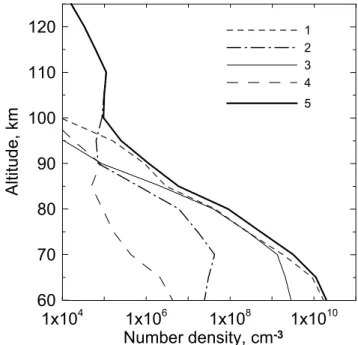
In Fig. 6 the altitude profile of the O2(X36g−, v=1) con-centration and the contributions of different channels of the O2(X36−g, v=1) population are shown. As can be seen from Fig. 6, ozone photolysis in the Hartley, Huggins and Chap-pius bands is the main channel of the O2(X36g−, v=1) pop-ulation up to 95 km, however, in the range 70–85 km the ab-sorption of solar radiation by oxygen at 689 and 762 nm gives almost the same contribution. Above 95 km ozone photoly-sis gives way to oxygen photolyphotoly-sis in the Shumann-Runge continuum and in the Lyman-α. As can be concluded from our calculations, vibrational excitation of O2in the reaction

of ozone with atomic oxygen (Table 5) is insignificant during daytime (curve 4 in Fig. 6).

1x10

1x10

1x10

1x10

Number density, cm

60

70

80

90

100

110

120

Altitude, km

1 2 3 4 5

Fig. 6.Altitude profile of the number densities of the molecules in the state O2(X36g−, v=1) calculated selectively for four main

non-LTE channels if only one channel has been taken into account for the conditions of experiment METEORS (Mlynczak et al., 2001) in accordance with our model: 1 – ozone photolysis in the Hartley, Huggins and Chappius bands; 2 – photolysis of O2in the

Shumann-Runge continuum and Lyman-α; 3 – absorption by O₂of solar ra-diation at 689 and 762 nm bands; 4 – reaction O3+O→O2(X36−g,

v)+O2(see Table 5); 5 – total density (all channels are taken into

account).

The altitude profiles of the concentration of O2(X36g−, v=1) were calculated with the purpose of solving the prob-lem of non-equilibrium radiation of H2O in the 6.3-µm band

in the middle atmosphere. The process of quasi-resonance V-V energy exchange between the first excited vibrational levels of the H2O and O2molecules is very fast; this is why

it is important to take into account this source of vibrational excitation of H2O(010) (Manuilova et al., 2001).

4 762-nm and 1.27-µm emissions in the middle atmo-sphere

We used our new model to calculate the concentrations of O2(a11g, v=0) and O2(b16g+, v=0) and, correspondingly, the intensities of the 1.27-µm and 762-nm emissions in the middle atmosphere.

1x104 2x104 5x104 1x105 2x105

5x103

Volume emission rate, photon

.

cm

_s

60 70 80 90 100 110 120

Altitude, km

60 70 80 90 100 110 120

1 2

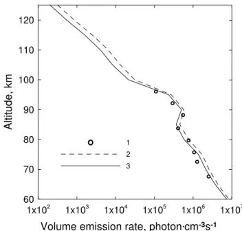
3

Fig. 7.Volume emission rate at 762 nm. Circles (1) – experimental data of METEORS (Mlynczak et al., 2001). Curves – calculations for the conditions of experiment METEORS: 2 – in accordance with the model of Mlynczak et al. (1993); 3 – in accordance with our model.

transfer between electronic states at collisions occur without vibrational excitation. Accordingly, only 17 processes re-main from more than 100 listed in Tables 1–5. This model to-tally corresponds to the model of Mlynczak et al. (1993). All calculations presented below have been made for both mod-els; the pure electronic model is called by us as the model of Mlynczak et al. (1993).

Figure 7 presents the comparison of the experimental data on the vertical profile of the volume emission rate at the wavelength of 762 nm (Mlynczak et al., 2001) and the cal-culations for the experimental conditions provided by our model and the model of only electronic kinetics.

In the same experiment (Mlynczak et al., 2001), the in-tensity of the 1.27-µm emission was measured simultane-ously with the 762-nm emission. In Fig. 8 the experimental data on the vertical profile of the volume emission rate at the wavelength of 1.27-µm are compared with the calculations for the experimental conditions provided by our model and the model of Mlynczak et al. (1993). For the entire altitude interval, the values of the volume emission rate at the wave-length of 1.27µm, calculated in accordance with our model, are lower than the results calculated in accordance with the model of Mlynczak et al. (1993). The discrepancy between the volume emission rates at 1.27µm, calculated in accor-dance with the electronic-vibrational kinetics model, and the pure electronic model is 15–60% at the region of 60–125 km.

1x102 1x103 1x104 1x105 1x106 1x107

Volume emission rate, photon.cm-3_s-1

60 70 80 90 100 110 120

Altitude, km

1

2

3

Fig. 8.Volume emission rate at 1.27µm. Circles (1) – experimental data of METEORS (Mlynczak et al., 2001). Curves – calculations for the conditions of experiment METEORS: 2 – in accordance with the model of Mlynczak et al. (1993); 3 – in accordance with our model.

5 Retrieval of the vertical ozone profile from the mea-sured intensity profiles of the 762-nm and 1.27-µm emissions

We will show that consideration of electronic-vibrational ki-netics is very important for the problem of ozone retrieval from the measurements of the intensity in the Atmospheric and IR Atmospheric bands of the O2molecule. For the

pur-pose of revealing which errors evolve due to the use of the pure electronic kinetics, we carried out the following numer-ical experiments.

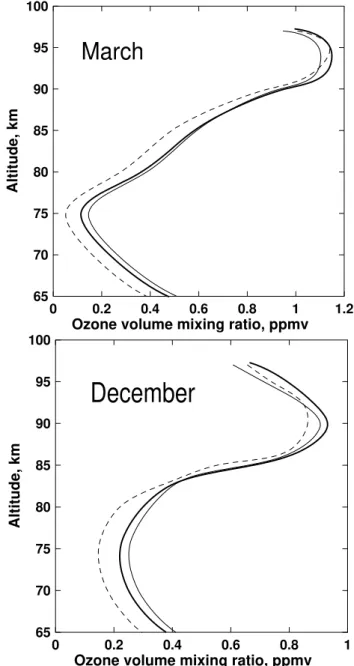
mixing ratio retrieved from the 762-nm emission, and for the 1.27-µm emission the retrieved ozone mixing ratio is two times smaller than the test one. For December, at 75 km the discrepancy reaches 14% for the ozone mixing ratio retrieved from 762-nm emission and 33% for the ozone mixing ratio retrieved from 1.27-µm emission. From the numerical exper-iment which was described above, it can be concluded, that in the framework of pure electronic kinetics the retrieval of the ozone mixing ratio from the 762-nm emission is prefer-able to the retrieval from the 1.27-µm emission.

The second numerical experiment is the interpretation of the atmospheric experiment on the retrieval of the vertical ozone profile from simultaneous measurements of the in-tensity in the Atmospheric and IR Atmospheric bands of the O2 molecule carried out in the experiment METEORS

(Mlynczak et al., 2001). Using our model and the model of Mlynczak et al. (1993), we have solved the inverse problem of the [O3] determination from the METEORS volume

emis-sion rates at 762 nm and 1.27µm presented in Mlynczak et al. (2001). Figure 10 presents the results of the retrieval of the ozone concentration.

Above 65 km, according to our model, the vibrational-electronic kinetics of the products of O3and O2 photolysis

play an important role in the mechanism of the formation of these emissions. As a result, above 65 km the retrievals of [O3] by our model and the model of Mlynczak et al. (1993)

differ significantly.

In accordance with the calculations for the model of Mlynczak et al. (1993), in the region near 85–90 km, the O3concentration retrieved from the intensity of the O2band

at 762 nm is 45–30% greater than the O3concentration

re-trieved from the intensity of the O2 band at 1.27µm (see

dashed lines in Fig. 10).

For our model the vertical [O3] profiles retrieved from both

emissions are closer to each other, and in the altitude range of 80–90 km the discrepancy is 20–17% (solid lines in Fig. 10). The [O3] value retrieved from the intensity of the 1.27-µm

band, in accordance with our model in the range of the local ozone peak at 80–90 km, is 40–15% as large as that obtained for the model of Mlynczak et al. (1993) (lines 3 and 4 in Fig. 10).

As can be seen from both numerical experiments (Figs. 9, 10), up to 90 km the differences between the ozone abun-dances retrieved in accordance with our model and the model of pure electronic kinetics of O3 and O2 photolysis from

the emission at 762 nm are much smaller than the corre-sponding difference between the ozone abundances retrieved in accordance with both models from the 1.27-µm emis-sion. Mlynczak et al. (1993) considered only populating O2(b16g+, v=0), using the total rate constant of collisions of O(1D) with O2. We considered the process of populating

the electronic-vibrational levels O2(b16g+, v=0, 1), using the same total rate constant, but taking into account the quantum yields of the O2(b16g+, v=0) and the O2(b16g+, v=1)

for-0 0.2 0.4 0.6 0.8 1 1.2

Ozone volume mixing ratio, ppmv 65

70 75 80 85 90 95 100

Altit

u

d

e

, km

March

0 0.2 0.4 0.6 0.8 1

Ozone volume mixing ratio, ppmv 65

70 75 80 85 90 95 100

Alti

tude, km

December

Fig. 9. Altitude profiles of ozone concentration retrieved from “measured” O2emissions at 762 nm (thin solid line) and 1.27µm

(dashed line) in accordance with pure electronic kinetics model. “Measured” volume emission rates at 762 nm and 1.27µm were calculated in accordance with electronic-vibrational kinetics model at using HRDI ozone profiles for March and December (thick solid line) (Marsh et al., 2002).

1x107 1x108 1x109 1x1010

Number density, cm

65 70 75 80 85 90 95

Altitude, km

1 2 3 4

Fig. 10.Altitude profiles of ozone concentration retrieved from si-multaneous observations of O₂emissions at 762 nm and 1.27µm in METEORS (Mlynczak et al., 2001). Retrievals in accordance with: our model – solid lines, model of Mlynczak et al. (1993) – dashed lines. Curves 1 and 2 – retrievals from measurement of emission at 762 nm O2(b16g+, v=0→X36g−, v=0). Curves 3 and

4 – retrievals from measurement of emission at 1.27µm O2(a11g,

v=0→X36g−, v=0).

Based on the results of ozone retrievals from emissions at 762 nm and 1.27µm, presented in Figs. 9 and 10, one can conclude that ozone abundance retrieval carried out in ac-cordance with the model of only electronic kinetics of O3

and O2photolysis (Mlynczak et al., 1993) from the emission

at 762 nm, which is formed by the transition from the state O2(b16g+), is preferable to retrieving the profiles of ozone abundance from the Infrared Atmospheric band of O2

emis-sion at 1.27µm, which is formed by the transition from the state O2(a11g). This conclusion is the opposite to the tra-ditional point of view but is not surprising, because in our model it was shown that the mechanism of populating the O2(a11g, v) states is much more complicated than that of populating the O2(b16+g, v) states (see Fig. 1 and Tables 1– 4).

It should be noted that we came to this assertion on the basis of the analysis of only two numerical experiments. The final conclusion about the errors introduced in the retrieved values of ozone concentrations when using the model of only electronic kinetics of O3 and O2 photolysis for retrieval of

the profiles of ozone concentration from the measurements in the bands at 762 nm and 1.27µm can only be made after analyzing a great deal of data (e.g. in the satellite experiment ODIN-OSIRIS both emissions are measured simultaneously during a long period of time; Murtagh et al., 2002).

1x107 1x108 1x109 1x1010

Number density, cm

65 70 75 80 85 90 95

Alt

it

ude, km

762 nm with CO2

762 nm without CO2 1270 nm with CO2

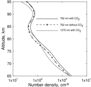
Fig. 11. Altitude profiles of ozone concentration retrieved from si-multaneous observations of O2emissions at 762 nm and 1.27µm in

METEORS (Mlynczak et al., 2001). Retrievals in accordance with our model: taking into account CO2altitude profile – solid lines,

with CO2mixing ratio equal to 0 – dashed lines.

It is interesting to point to the influence of CO2abundance

on the retrieval of ozone concentrations from the measure-ments in the band at 762 nm which is connected with the high value of the rate constant of reaction of deexcitation of O2(b16g+, v=0) by CO2, whereas the CO2concentration

does not influence the retrieval of ozone concentration from the measurements in the band at 1.27µm (Fig. 11). For the calculations presented in Fig. 11 we used the CO2altitude

profile from Kauffmann et al. (2002), which gives a signifi-cant decrease in the CO2volume mixing ratio above 75 km.

Comparison of the ozone concentrations retrieved from the measurements in the band at 762 nm, taking into account the [CO2] altitude profile and with CO2mixing ratio equal to 0

in the whole altitude region shows, in the framework of our model, a sensitivity of ozone concentrations retrieval to the [CO2] altitude profile below 90 km (Fig. 11).

6 Conclusions

2. Above 65 km the previous model of electronic kinetics of the excited products of the ozone and oxygen pho-tolysis should be replaced by the model of electronic-vibrational kinetics.

3. The proposed model allows for calculation not only of vertical profiles of the O2(a11g, v=0) and O2(b16g+, v=0) concentrations, but also of the profiles of [O2(a11g, v≤5)] and [O2(b16g+, v=0, 1, 2)]. Cor-respondingly, in accordance with our model, not only the intensity of the 1.27-µm and 762-nm emissions, but also the intensity of emissions formed by transi-tions from electronically-vibrationally excited levels, such as O2(b16g+, v=1)→O2(X36g−, v=0) at 689 nm and O2(b16+g, v=2)→O2(X36−g, v=0) at 629 nm, can be calculated in the middle atmosphere. The model also enables us to calculate the number densities of O2

molecules in the ground electronic state with the vibra-tional quantum numbers from 1 to 35.

4. With the consideration of the electronic-vibrational ki-netics of the excited products of the ozone and oxygen photolysis, the discrepancy between the altitude profiles retrieved from the simultaneously measured intensities of the 762-nm and 1.27-µm emissions in the experi-ment METEORS (Mlynczak et al., 2001) becomes sig-nificantly smaller than it was for only the electronic ki-netics model. The developed model, in principle, gives an opportunity to retrieve the ozone density profiles from different emissions formed by transitions from electronically-vibrationally excited levels of singlet O2

molecules in the middle atmosphere.

5. Based on the results of the numerical experiments on ozone retrievals (using the experimental ozone mix-ing ratio profiles from HRDI experiment (Marsh et al., 2002) and simultaneously measured emissions at 762 nm and 1.27µm in the experiment METEORS (Mlynczak et al., 2001)), one can conclude that in the case of the pure electronic kinetics model the ozone abundance retrieval from the emission at 762 nm is preferable to retrieving the profiles of ozone abundance from the infrared Atmospheric band of O2emission at

1.27µm. Using the 1.27-µm emission measurements for ozone concentration retrieval above 65 km is incor-rect if the interpretation of experiments is carried out in accordance with models of pure electronic kinetics of O3and O2photolysis.

Acknowledgements. The authors thank T. G. Slanger (SRI Interna-tional, California) and V. I. Fomichev (York University, Toronto) for providing urgently needed information and for fruitful discussions and also post-graduate student V. A. Kuleshova (St. Petersburg State University, St. Petersburg) and M. A. Shelyakhovskaya for techni-cal assistance. This work was partly supported by RFBR grants N 02-05-65259 and 05-05-65318.

Topical Editor U.-P. Hoppe thanks N. N. Shefov and another ref-eree for their help in evaluating this paper.

References

Allen, M. and Frederick, J. E.: Effective photodissociation cross sections for molecular oxygen and nitric oxide in the Schumann-Runge bands, J. Atmos. Sci., 39, 2066–2075, 1982.

Amimoto, S. T. and Wiensfeld, J. R.: O2(b16+g)production and

deactivation following quenching of O(1D) in O3/O2mixtures,

J. Chem. Phys., 72, 3899–3903, 1980.

Atkinson, R., Baulch, D. L., Cox, R. A., Hampson Jr., R. F., Kerr, J. A. (Chairman), and Troe, J.: Evaluated kinetic and photo-chemical data for atmospheric chemistry supplement VI, IUPAC Subcommittee on Gas Kinetic Data Evaluation for Atmospheric Chemistry, J. Phys. Chem. Ref. Data, 26, 1329–1497, 1997. Ball, S. M., Hancock, G., and Winterbottom, F.: Product channels in

the near-UV photodissociation of ozone, Faraday Discuss., 100, 215–227, 1995.

Balakrishnan, N. and Billing, G. D.: Quantum-classical reaction path study of the reaction O(3P)+O3(1A1)→2O2(X36g−), J.

Chem. Phys., 104, 23, 9482–9494, 1996.

Billing, G. D. and Kolesnick, R. E.: Vibrational relaxation of oxy-gen. State to state rate constants, Chem. Phys. Lett., 200, 382– 386, 1992.

Braithwaite, M., Davidson, J. A., and Ogryzlo, E. A: O2(16g+)

re-laxation in collisions. I. The influence of long range forces in the quenching by diatomic molecules, J. Chem. Phys., 65, 771–778, 1976.

Breig, E. L.: Statistical model for the vibrational deactivation of molecular by atomic oxygen, J. Chem. Phys., 51(10), 4539– 4547, 1969.

Bucholtz, A., Skinner, W. R., Abreu, V. J., and Hays, P. B.: The dayglow of the O₂Atmospheric band system, Planet. Space Sci., 34, 1031–1035, 1986.

Coletti, C. and Billing, G. D.: Vibrational energy transfer in molec-ular oxygen collisions, Chem. Phys. Lett., 356, 14–22, 2002. DeMajistre, R., Yee, J.-H., and Zhu, X.: Parameterizations of

oxy-gen photolysis and energy deposition rates due to solar energy absorption in the Schumann-Runge continuum, Geophys. Res. Lett., 28(16), 3163–3166, 2001.

DeMore, W. B., Golden, D. M., Hampson, R. F., Howard, C. J., Kolb, C. E., and Molina, M. J.: Chemical kinetics and photo-chemical data for use in stratospheric modeling, JPL Publication, 97-4, 1–128, 1997.

Dylewski, S. M., Geiser, J. D., and Houston, P. L.: The energy distribution, angular distribution, and alignment of the O(1D) fragment from the photodissociation of ozone between 235 and 305 nm, J. Chem. Phys, 115, 7460–7473, 2001.

Green, J. G, Shi, J., and Barker, J. R.: Photochemical kinetics of vibrationally excited ozone produced in the 248 nm photolysis of O2/O3mixtures, J. Phys. Chem. A, 104, 6218–6226, 2000.

Hady-Ziane, S., Held, B., Pignolet, P., Peyrous, R., and Coste, C.: Ozone generation in an oxygen-fed wire-to-cylinder ozonizer at atmospheric pressure, J. Phys. D: Appl. Phys., 25, 677–685, 1992.

Hwang, E. S., Bergman, A., Copeland, R. A., and Slanger, T. G.: Temperature dependence of the collisional removal of O2(b16+g,

v=1 & 2) at 110–260 K, and atmospheric applications, J. Chem. Phys., 110, 18–24, 1999.

Kalogerakis, K. S., Copeland, R. A., and Slanger, T. G.: Collisional removal of O2(b16g+, v=2, 3), J. Chem. Phys., 116, 4877–4885,

2002.

Kalogerakis, K. S., Copeland, R. A., and Slanger, T. G.: Vibrational energy transfer in O2(X36−g, v=2, 3)+O2collisions at 330 K, J.

Chem. Phys., 123, 044303, doi:10.1063/1.1982788, 2005. Kaufmann, M., Gusev, O. A., Grossmann, K. U., Roble, R. G.,

Ha-gan, M. E., Hartsough, C., and Kutepov, A. A.: The vertical and horizontal distribution of CO2densities in the upper mesosphere

and lower thermosphere as measured by CRISTA, J. Geophys. Res. D, 107, 8182, doi:10.1029/2001JD000704, 2002.

Keating, G. M., Pitts, M. C., and Chen, C.: Improved reference models for middle atmosphere ozone Book: Middle Atmosphere Program, Handbook for MAP, 31, 37–49, 1989.

Klais, O., Laufer, A. H., and Kurylo, M. J.: Atmospheric quenching of vibrationally excited O2(a11g), J. Chem. Phys., 73, 2696–

2699, 1980.

Klingshirn, H. and Maier, M.: Quenching of the O2(a11g)state in

liquid isotopes, J. Chem. Phys., 82, 714–719, 1985.

Koppers, G. A. A. and Murtagh, D. P.: Model studies of the influence of O2photodissociation parameterizations in the

Schumann-Runge bands on ozone related photolysis in the upper atmosphere, Ann. Geophys., 14, 68–79, 1996,

http://www.ann-geophys.net/14/68/1996/.

Krupenie, P. H.: The spectrum of Molecular Oxygen, J. Phys. Chem. Ref. Data, 1, 423–521, 1972.

Lee, L. C. and Slanger, T. G.: Observation on O(1D→3P) and O2(b16+g→X36g−) following O2photodissociation, J. Chem.

Phys., 69, 4053–4060, 1978.

Llewellyn, E. J. and McDade, I. C.: A reference model for atomic oxygen in the terrestrial atmosphere, Adv. Space Res., 18, 209– 226, 1996.

Lopez-Gonzalez, M. J., Lopez-Moreno, J. J., and Rodrigo, R.: The altitude profile of the infrared atmospheric system of O2in

twi-light and early night: derivation of ozone abundance’s, Planet. Space Sci., 40, 1391–1397, 1992.

Lopez-Puertas, M., Zaragoza, G., Kerridge, B. J., and Taylor, F. W.: Non-local thermodynamic equilibrium model for H₂O 6.3 and 2.7µm bands in the middle atmosphere J. Geophys. Res. D, 100, 9131–9147, 1995.

Manuilova, R. O., Yankovsky, V. A., Semenov, A. O., Gusev, O. A., Kutepov, A. A., Sulakshina, O. N., and Borkov, Yu. G.: Non-equilibrium emission of the middle atmosphere in the IR ro-vibrational water vapor bands, Atmos. Oceanic Opt., 14, 864– 867, 2001.

Marsh, D. R., Skinner, W. R., Marshall, A. R., Hays, P. B., Ortland, D. A., and Yee, J.-H.: High resolution Doppler imager obser-vations of ozone in the mesosphere and lower thermosphere, J. Geophys. Res. D, 107(D19), 4390, doi:10.1029/2001JD001505, 2002.

Michelsen, H. A., Salawitch, R. J., Wennberg, P. O., and Anderson, J. G.: Production of O(1D) from photolysis of O3, Geophys. Res.

Lett., 21, 2227–2230, 1994.

Mlynczak, M. G., Solomon, S. C., and Zaras, D. S.: An updated model for O2(11g)concentrations in the mesosphere and lower

mesosphere and implications for remote sensing of ozone at 1.27µm, J. Geophys. Res. D, 98, 18 639–18 648, 1993. Mlynczak, M. G. and Marshall, B. T.: A reexamination of the role

of solar heating in the O2atmospheric and infrared Atmospheric

bands, Geophys. Res. Lett., 23, 657–660, 1996.

Mlynczak, M. G., Morgan, F., Yee, J.-H., Espy, P., Murtagh, D., Marshall, B. T., and Schmidlin, F.: Simultaneous measurements of the O₂(a11g)and O2(b16g+)airglows and ozone in the

day-time mesosphere, Geophys. Res. Lett., 28, 999–1002, 2001. Murtagh, D., Frisk, U., Merino, F., et al.: An overview of the Odin

atmospheric mission, Can. J. Phys., 80, 309–319, 2002. Olemskoy, I. V.: Updating of algorithm of allocation structural

fea-tures, Vestn. S. – Petersburg Univ., Ser. 10: Prikl. Matem., 55–64, 2006.

Pejakovic, D. A., Wouters, E. R., Phillips, K. E., Slanger, T. G., Copeland, R. A., and Kalogerakis, K. S.: Collisional removal of by O₂at thermospheric temperatures. J. Geophys. Res. A, 110, 03308, doi:10.1029/2004JA010860, 2005.

Polack, L. S.: Non equilibrium chemical kinetics. Science Press, Moscow, 1979.

Reddmann, T. and Uhl, R.: The H Lyman-αactinic flux in the mid-dle atmosphere, Atmos. Chem. Phys., 3, 225–231, 2003, http://www.atmos-chem-phys.net/3/225/2003/.

Rodrigo, R., Lopez-Moreno, J. J., Lopez-Puertas, M., Moreno, F., and Molina, A.: Neutral atmospheric composition between 60 and 220 km: a theoretical model for mid-latitudes, Planet. Space Sci., 34, 723–743, 1986.

Sica, R. J. and Lowe, R. P.: Inferring middle atmospheric ozone height profiles from ground-based measurements of molecules oxygen emissions rates, 2. Comparison with the O2(a11g)(0,

1) band measurements at sunset, J. Geophys. Res. D, 98, 1051– 1055, 1993a.

Sica, R. J. and Lowe, R. P.: Inferring middle atmospheric ozone height profiles from ground-based measurements of molecules oxygen emissions rates, 3. Can twilight measurements of the At-mospheric band be used to retrieve an ozone density profile, J. Geophys. Res. D, 98, 1057–1067, 1993b.

Skinner, W. R. and Hays, P. B.: Brightness of the O2Atmospheric

bands in the daytime thermosphere, Planet. Space Sci., 33, 17– 22, 1985.

Slanger, T. G.: Studies on highly vibrationally-excited O2,

AIAA-97-2502, 32nd Thermophysics Conference, 23–25 June 1997/At-lanta, GA1997, 1997.

Slanger, T. G. and Copeland, R. A.: Energetic oxygen in the up-per atmosphere and the laboratory, Chem. Rev., 103, 4731–4765, 2003.

Sparks, R. K., Carlson, L. R., Snobatake, K., Kowalczyk, M. L., and Lee, Y.T.: Ozone photolysis: A determination of the electronic and vibrational state distributions of primary products, J. Chem. Phys., 72, 1401–1402, 1980.

Streit, G. E., Howard, C. J., Schmeltekopf, A. L., Davidson, J. A., and Schiff, H. I.: Temperature dependence of O(1D) rate con-stants for reactions with O2, N2, CO2, O3, H2O, J. Chem. Phys.,

65, 11, 4761–4764, 1976.

Svanberg, M., Pettersson, J. B. C., and Murtagh, D.: Ozone pho-todissociation in the Hartley band: A statistical description of the ground state decomposition channel O2(X36g−)+ O(3P), J.

Chem. Phys., 102, 8887–8896, 1995.

Photodis-sociation of ozone in the Hartley band: Fluctuation of the vibra-tional state distribution in the O2(a11g, v) fragment, J. Chem.

Phys., 103, 7946–7955, 1995.

Thomas, R. J., Barth, C. A., Rusch, D. W., and Sanders, R. W.: Solar mesosphere explorer near-infrared spectrometer: Measure-ments of 1.27µm radiances and the interference of mesospheric ozone, J. Geophys. Res., 89, 9569–9580, 1984.

Tully, J. C.: Collision complex model for spin forbidden reactions: Quenching of O(1D) by N2, J. Chem. Phys., 61, 61–68, 1974.

Valentini, J. J., Gerrity, D. P., Phillips, D. L., Nieh, J.-C., and Tabor, K. D.: CARS spectroscopy of O2(a11g)from the Hartley band

photodissociation of O3: Dynamics of the dissociation , J. Chem.

Phys., 86, 6745–6756, 1987.

Webster III, H. and Bair, E. J.: Ozone ultraviolet photolysis. IV. O2*+O(3P) vibrational energy transfer, J. Chem. Phys., 56,

6104–6108, 1972.

Wild, E., Klingshirn, H., and Maier, M.: Relaxation of the a11g

state on pure liquid oxygen and in liquid mixtures of(16)O2and (18)_O

2, J. Photochem., 25, 134–143, 1984.

Yankovsky, V. A.: Electronic-vibrational relaxation of O₂(b16+_g, v=1,2) at collisions with ozone and molecular and atomic oxy-gen, (in Russian), Khim. Fiz., 10, 291–306, 1991.

Yankovsky, V. A. and Kuleshova, V. A.: Photodissociation of ozone in Hartley band. Analytical description of quantum yields of O2(a11g, v=0-3) depending on wave length, (in Russian),

At-mos. Oceanic Opt., 19, 576–580, 2006.

Yankovsky, V. A. and Manuilova, R. O.: New self-consistent model of daytime emissions of O2(11g) and O2(b16g+) in the

mid-dle atmosphere. Retrieval of vertical ozone profile from the mea-sured intensity profiles of these emissions, Atmos. Oceanic Opt., 16, 536–540, 2003.