A NEW EFFICIENT NONLINEAR PROGRAMMING BASED METHOD
FOR BRANCH OVERLOAD ELIMINATION
Heder D. Abrantes
∗Carlos A. Castro
∗∗DSEE/FEEC/UNICAMP, P.O. Box 6101, 13081-970 Campinas SP, Brazil
ABSTRACT
A simple and efficient method for eliminating branch overloads in power systems is presented in this paper. The overloads are eliminated by corrective control ac-tions, which are defined through the use of an efficient and accurate nonlinear programming method. Genera-tion rescheduling (GR) and load shedding (LS) are the main controls used. The idea of adaptative local op-timization (ALO) is introduced. The computation of appropriate GR using ALO becomes a very efficient pro-cess. LS is used as a last resort, when further GR is no longer possible. Heuristics are added in order to speed up the computation process and to take into account some practical aspects of power systems operation into it. A special procedure is carried out in case of critical situations, where emergency control actions are defined. The method’s general idea is to keep the new secure operating point as close as possible to the original one, while minimizing the amount of LS. The method can be a helpful tool for operation planning studies, secu-rity analysis and reliability evaluation of power systems. Simulations have been carried out for small test to large real life systems in order to show the efectiveness of the proposed method.
KEYWORDS: Power system security analysis, power
sys-tem operation, violations elimination, nonlinear pro-gramming.
Artigo submetido em 30/11/00
1a. Revis˜ao em 22/11/01; 2a. revis˜ao em 25/04/02
Aceito sob recomenda¸c˜ao do Ed. Assoc. Prof. Jos´e Luiz R. Pereira
RESUMO
Neste artigo ´e proposto um m´etodo simples e eficiente para eliminar sobrecargas em ramos de redes el´etricas de potˆencia. Essas sobrecargas s˜ao eliminadas atrav´es de a¸c˜oes de controle corretivo que s˜ao definidas atrav´es do uso de um m´etodo preciso e eficiente de programa¸c˜ao n˜ao-linear. Redespacho da gera¸c˜ao e corte de carga s˜ao os principais controle utilizados. A id´eia de otimiza¸c˜ao local adaptativa ´e introduzida. O c´alculo dos redespa-chos de gera¸c˜ao utilizando a otimiza¸c˜ao local adapta-tiva ´e realizado de maneira muito eficiente. O corte de carga ´e utilizado como ´ultima alternativa, nas situa¸c˜oes em que o redespacho da gera¸c˜ao n˜ao ´e mais poss´ıvel. Heur´ısticas s˜ao acrescentadas a fim de tornar o procedi-mento computacional mais r´apido e de levar em conta alguns aspectos pr´aticos da opera¸c˜ao de redes el´etricas de potˆencia. Um procedimento especial ´e executado no caso de situa¸c˜oes cr´ıticas, em que a¸c˜oes de controle de emergˆencia s˜ao realizadas. A id´eia geral do m´etodo ´e fazer com que o novo ponto de opera¸c˜ao segura esteja o mais pr´oximo poss´ıvel de ponto de opera¸c˜ao original, al´em de minimizar o montante de corte de carga. O m´etodo proposto pode ser uma ferramenta ´util para es-tudos de planejamento, an´alise de seguran¸ca e avalia¸c˜ao da confiabilidade de sistemas de potˆencia. Foram reali-zadas simula¸c˜oes para v´arias redes, inclu´ındo redes teste de pequeno porte e redes de grande porte reais, a fim de mostrar a efic´acia do m´etodo proposto.
PALAVRAS-CHAVE: An´alise de seguran¸ca de sistemas de
1
INTRODUCTION
Power systems operating conditions undergo frequent changes due to the occurence of outages and demand variations. These changes may result in one or more branch (transmission lines or transformers) MW over-loads. In order to keep the system within secure operat-ing conditions, corrective control actions must be taken so as to eliminate such overloads. Among the possible corrective control actions are generation rescheduling, interchange adjustments, phase shifters adjustments, network switching and load shedding (Wood and Wol-lenberg, 1984). Corrective control actions to eliminate overloads must be determined within a small time frame, specially in case of a real time control environment. They can also be determined by off-line calculations in order to provide a control strategy to be used in case of emergencies.
Several overload elimination methods have been pro-posed in the literature. In (Wood and Wollenberg, 1984; Castro and Bose, 1993; Castro and Bose, 1994) gener-ation rescheduling methods based on genergener-ation shift factors were proposed. Heuristics were added in order to determine the controls to be used and to take into account some practical aspects of power systems opera-tion. In (Medicherlaet alii, 1979) bus injection changes were defined so as to decrease branch currents based on sensitivity factors. Nonlinear programming methods have also been proposed for finding coordinated control actions to eliminate overloads (Shandilyaet alii, 1993). Optimization techniques are usually expensive from a computational standpoint. This cost increases with the size of the system. In (Shandilyaet alii, 1993) the idea of local optimization (LO) is introduced. A fixed sized region (hereafter called work region) around the over-loaded branch (or branches) is previously defined and corrective control actions are chosen within this region. Thus, the size of the problem to be solved is practically independent of the system size. Also, a scheme is pro-posed in an attempt to obtain minimum load shedding with maximum efficiency.
In this paper a nonlinear programming based method is proposed. Generation rescheduling and load shedding will be used as controls. The idea of LO (Shandilya
et alii, 1993) has been extended toadaptive local opti-mization(ALO). Once the work region has been defined in LO, available generators for rescheduling may not be found. In ALO, the work region is defined so that gen-erators with large sensitivities with respect to eliminat-ing the overloads are always included. In (Shandilyaet alii, 1993) all buses outside the work region are consid-ered as slack buses (their states keep unchanged after
control actions are taken into effect). Of course this is an approximation, since their states actually change after control actions are taken. In ALO, sparse vec-tor techniques (Tinneyet alii, 1985) are used and exact results are obtained with minimum computational ef-fort. In addition, heuristics are added for increasing the overall efficiency of the computation process and cop-ing with some practical aspects of the problem. Finally, emergency control measures are also allowed for critical overload cases for which usual generation rescheduling and load shedding are not sufficient. This provides the operator with a feasible solution for the problem, even though the system may have been driven farther away from its original operating point.
2
PROBLEM FORMULATION
In order to alleviate the existing overloads, a nonlinear optimization problem is formulated so as to minimize a quadratic function which includes the differences be-tween the current MW power flows and their respective limits. This function will have as many terms as the number of overloaded branches. Let OL be the set of overloaded branches. Thus, the objective function is:
f(x) = X
ℓ∈OL
(Pℓ−Pmax ℓ ·sf)
2
(1)
where sf is a safety factor and x is the state variable vector (voltage magnitudes and phase angles). Func-tionf(x) can be minimized by changing bus MW power injections (generator rescheduling and load shedding). They are regarded as control variables. The constraints for this problem are:
g(x,u) =0 (2)
h(x,u)≤0 (3)
umin
≤u≤umax
(4)
whereuis the set of control variables.
Eq. (2) corresponds to the set of load flow equa-tions. For practical purposes, MW power flows through branches depend basically on their phase angle spreads. Thus, equations that relate real powers and phase an-gles will are considered only. More specifically, the real power balance equation of the fast decoupled load flow formulation (Stott and Alsa¸c, 1974) is used. Cases for which power flows are affected by voltages magnitudes are appropriately taken care of in the solution process, as it will become clear in Sec. 3.
not violated at the solution point (most branches are not overloaded). Besides, the objective function specif-ically aims to satisfying the active constraints. As for bus voltage magnitudes, their limits may be considered in an appropriate manner in the solution process (Sec. 3). Therefore, (3) need not to be included in the basic formulation.
Eq. (4) takes into account the control variable lower and upper limits. In this case, only real power bus injections (generator rescheduling and load shedding) were consid-ered. Finally, the problem is formulated as:
f(θ) = X
ℓ∈OL
(Pℓ−Pmax ℓ ·sf)
2
(5)
subject to
g(θ,Ps) =Ps−Pc
(θ) =0 (6)
Pmin
≤Ps
≤Pmax
(7)
where θ is the nodal phase angle vector, and Ps and
Pc
are respectively the scheduled and calculated nodal real power injections. The elements of vector Pc
are computed by:
Pc i =Vi
X
j∈Ai
Vj(Gijcosθij+Bijsinθij)
whereVi is the voltage magnitude at busi,Gij andBij
are elements of the admittance matrix, andAi is a set containing busiplus the buses directly connected to it.
In this paper equations (5)–(7) are solved by a projected steepest descent method (Bazaraa and Shetty, 1993) wherePsis the vector of independent variables andθis
the vector of the dependent variables. See Appendix A for further details.
As a consequence of the utilization of LO, the set of constraints (6) is formed by a small number of load flow equations (depending on the size of the work region). When ALO is used this set is formed by the load flow equations for all buses. However, they are solved as effi-ciently as in LO with the use of sparse vector techniques, with greater accuracy, as mentioned before.
The solution of the problem is obtained through a step by step procedure, each of which having a different con-trol strategy. The concon-trol strategies defined are the fol-lowing:
(1) generation rescheduling only;
(2) load shedding at the receiving end bus of the over-loaded branches;
(3) load shedding at the buses to which power is being fed from the receiving end bus of the overloaded branches (first tier);
(4) change power injection (either rescheduling or load shedding) at buses located up to the second tier;
(5) change power injection (either rescheduling or load shedding) at buses located up to the third tier; and so on.
During the iterative process a specific control strategy is selected depending on the system condition at that iter-ation. The first three strategies have been proposed by (Shandilyaet alii, 1993). The other ones are performed in case of persisting overloads and are referred to as emergency control measures. They assure that a feasible solution will be found in case of severe overloads. The determination of emergency control measures is very im-portant to operators, specially when dealing with severe and hard to solve overload problems.
3
PROPOSED ALGORITHM
The complete procedure for alleviating branch overloads is as follows:
1 Perform load flow calculations using the sched-uled load and generation information. Set strategy pointersp= 1 and outer iteration counter oc= 1;
2 Calculate branch flows. If no overloads are found, go to step 12. If sp > spmax, stop. Else set inner
iteration counteric= 1;
3 Calculate the value of the objective function f0 at
the current operating point;
4 If sp >1, determine the buses to be processed ac-cording to the current strategy, compute the respec-tive elements ofλusing Eq. (12) and go to step6;
with small sensitivities are found in two consecu-tive tiers. For each generator that is found, the corresponding value of vector λ is computed. In
case the generator is not included as a control, the respective position is zeroed;
6 Calculate the conjugate of the direction given byλ,
that is,S=−λ;
7 Take into account the limits of the control variables, computing the projection of the gradients onto the bounds of the independent variables. The elements of vectorSare redefined as:
sj=
0
ifPmax
j −Pj = 0 andsj>0
ifPj−Pmin
j = 0 and sj<0 sj otherwise
8 Calculate the maximum step sizetmsuch that:
tm= min
j
( min
sj>0
Pjmax−Pj
sj
,min
sj<0 "
Pjmin−Pj
sj
#)
9 Compute the optimum step size t∗ (0 ≤ t∗ ≤ tm)
using cubic fit (see Appendix B for more details). Calculate ∆P = t∗S. Update power injections Ps
= Ps
+∆P. Vector ∆P can include genera-tion rescheduling and/or load shedding, depending on the current strategysp;
10 Calculate the objective function value,f1. If f1 ≤ ǫ1 or [(f1−f0)/f1] ≤ǫ2 go to11. Otherwise,
in-crement inner iteration counter ic=ic+ 1 and go to step4;
11 Perform load flow calculations for the new genera-tion and load schedule. Set counters oc = oc+ 1 andsp=sp+ 1. Go to step2;
12 Compute the power injection at the slack bus. In case it is outside bounds, curtail load at the slack bus itself and/or at buses which are fed from the slack bus. The amount of load shedding is equal to the limit violation. Else stop.
4
HEURISTICS
The following heuristics were added to increase efficency and to take into account some practical aspects related to the overload elimination problem.
• Step2: in many cases it is possible that t∗ be
de-termined so as to zero the objective function, that is, the control actions are expected to successfully eliminate the overloads. However, after perform-ing load flow calculations one can find out that the
overloads have not been eliminated, but only allevi-ated. This occurs due to the utilization of the real part (P–θ) of the load flow equations in the opti-mization process. In case this situation occurs, set
sp=sp−1. Decreasing spimplies in performing another iteration by using the same control strategy as in the previous one, and the error is corrected;
• Step2: ifoc >1 and new overloaded branches are detected (those that appeared only after control ac-tions have been taken) such that the value of the ob-jective function increases, steps3–10are performed considering only the new overloaded branches for computing the objective function. After the new overloads had been eliminated, all controls used at this specific step are flagged. These controls cannot be changed in further iterations so that the same new overloads appear;
• Step9: in case the derivative of the objective func-tion evaluated att=tm
is less or equal to zero, set
t∗=tm
. Its negative sign indicates that the objec-tive function is still decreasing when some control limit has been reached. In this case some computa-tion savings are achieved;
• Step 11: if the load flow calculations do not con-verge, set the controls back to their previous values in the reverse order they appeared until convergence is obtained.
5
GENERAL COMMENTS
It follows general comments regarding the implementa-tion of the proposed method.
• The elements of vectorλin steps 4and5are
effi-ciently computed by using sparse vector techniques. Vector∂f /∂θis sparse, so fast forward substitution
can be performed. If a small number of elements of
λ is required, fast back substitution can be
per-formed;
• The threshold of step5is defined as a percentage of either the largest lagrangean multiplier related to the terminal buses of the overloaded branches or the lagrangean multiplier related to the first generator found;
• Tolerancesǫ1 andǫ2 are arbitrarily chosen. In this
paper ǫ1 = 10−6 and ǫ2 = 10−2 were used with
good final results.
phase angle coupling (Sec. 2). This feature of the problem allows the use of first order optimization methods, such as the steepest descent method used in this paper. The usually undesirable character-istics of first order methods, such as slow conver-gence, are not critical in this case. Nevertheless, the idea of adaptive local optimization can be used in conjunction with any optimization method, such as the second order Newton method (Sunet alii, 1984) and the interior point method (Ponnambalam et alii, 1991).
6
RESULTS OF SIMULATIONS
The simulation results shown in this pa-per are restricted to two power systems, namely the IEEE 300 bus, 411 branch system (http://www.ee.washington.edu/research) and a 904 bus, 1283 branch system which corresponds to a reduced version of the Southwestern USA system.
6.1
ALO versus LO
Table 1 shows a comparison between the concepts of ALO and LO using the 904 bus system. Branch 849– 851 is overloaded (original flow is 523.07 MW, limit set to 520.00 MW).
Table 1: ALO versus LO
ALO LO
oc,i 1, 1 2, 1 1, 1 2, 1
sp 1 1 1 2
control bus 17, 18(*) 17, 18(*)
- 849(*)
tier 3 3 - 0
control ac-tion
−23.13(r); −23.13(r)
−0.85(r); −0.85(r)
- 40.18(l)
power flow 520.11 520.00 523.07 519.76 (*) bus that limitedtm; (r) rescheduling;
(l) load shedding
In the case of LO, the work region was defined with 2 tiers, as suggested in (Shandilya et alii, 1993). In this case, no rescheduling was possible since there were no generators within the work area. The next step is to curtail load at the terminal bus of the overloaded branch. By using ALO, generators at the third tier were found and were able to eliminate the overload without load shedding. Generators 17 and 18 have the same sensitivities, resulting in identical rescheduling.
6.2
Multiple overloads
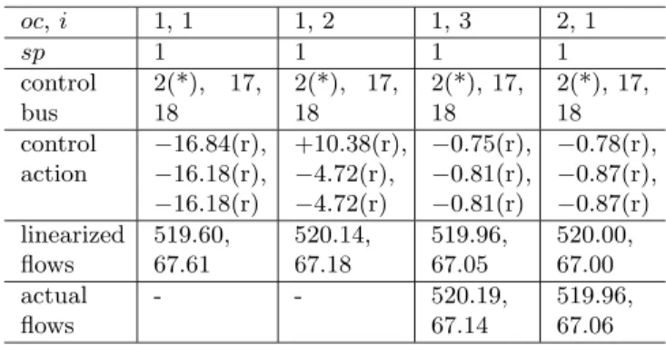
Table 2 shows simulation results for a double overload at branches 851–849 (original flow is 523.07 MW, limit set to 520.00 MW) and 849–890 (original flow is 70.36 MW, limit set to 67.00 MW) of the 904 bus system.
Table 2: Two overloads
oc,i 1, 1 1, 2 1, 3 2, 1
sp 1 1 1 1
control bus
2(*), 17, 18
2(*), 17, 18
2(*), 17, 18
2(*), 17, 18 control
action
−16.84(r), −16.18(r), −16.18(r)
+10.38(r),
−4.72(r), −4.72(r)
−0.75(r), −0.81(r), −0.81(r)
−0.78(r), −0.87(r), −0.87(r)
linearized flows
519.60, 67.61
520.14, 67.18
519.96, 67.05
520.00, 67.00 actual
flows
- - 520.19,
67.14
519.96, 67.06
After three inner iterations, control actions are taken so as to eliminate the overloads. However, by solving the load flow equations, it is found that the overloads are still present (though smaller than the original ones). Control actions are defined within an inner iteration by linearized calculations. There may be a difference be-tween the expected flows and the ones calculated by solving the load flow equations. Another external it-eration is necessary to finally eliminate the violation. In fact, it can be seen that there is a small overload left in branch 849-890. However, the stopping criteria is met, that is, the objective function is less or equal to ǫ1.
6.3
New overloads
Table 3 shows the results of a simulation of an overload at branch 849–851 (original flow is 523.07 MW, limit set to 520.00 MW) of the 904 bus system. Branch 851–824 (original flow is 78.26 MW, limit set to 80 MW) has also been monitored since it becomes overloaded after some control actions.
Table 3: New overload
oc sp control buses
overload considered
control action
actual flows
1 1 17;
18(*)
849-851 -23.13(r); -23.13(r)
520.11; 84.45
2 1 2(*); 17; 18
851-824 -9.01(r); 14.51(r); 14.51(r)
521.84; 79.84
3 1 - 849-851 - 521.84;
79.84 4 2 849(*) 849-851 24.10(l) 519.85;
81.41 5 2 824(*) 851-824 5.13(l) 520.43;
79.96 6 2 849(*) 849-851 5.64(l) 519.97;
80.32 7 2 824(*) 851-824 1.18(l) 520.10;
79.99
6.4
Emergency control measures
Table 4 shows the results provided by the proposed method for the IEEE 300 bus system. Branch 2–8 (orig-inal flow is 365.11 MW, limit set to 350 MW) is over-loaded.
Table 4: Extreme control mesures
oc 1 2 3 4
sp 1 2 3 4
control buses
7002(*) 8(*) - 7003, 9, 13, 15(*) control
action -23.00(r)
10.00(l) - -15.83(r), 4.92(l), 5.62(l), 15.69(l) actual
flows
357.74 353.37 353.37 349.86
In the first iteration generator 7002 is rescheduled down to its lower limit. In iteration 2, receiving end bus num-ber 8 undergoes load shedding. In iteration 3, buses fed from bus 8 (first tier) are checked and no load shedding is possible, however, the overload is still in effect. Iter-ation 4 constitutes an emergency control measure, that is, generation rescheduling and load shedding is allowed also for buses belonging up to the third tier, and the overload is eliminated through rescheduling of the gen-erator at bus 7003 and load shedding at buses 9, 13 and 15.
6.5
Performance aspects
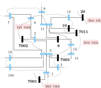
Some performance aspects will be discussed based on the same simulation shown in Section 6.4. In the first outer iteration (oc= 1) generator rescheduling was al-lowed only. The search for generators started from the terminal buses of the overloaded branch and ended up in the third tier, as shown in Figure 1. Generators 8, 7002, 7003, 10, 7011, 7001 and 20 were found. All of them, except generator 7002 either had small sensitivi-ties or could not be rescheduled due to their particular generation limits. Therefore, the work region consisted of generator bus 7002 and terminal buses 2 and 8. In or-der to find out the work region (and also vectorλ) one
fast forward (for the factorization path corresponding to buses 2 and 8) and six fast back (for the factoriza-tion paths corresponding to each one of the generators) substitutions were performed.
In all further iterations only one fast forward and one fast back substitutions had to be performed for obtain-ingλ. Of course, the factorization paths were different
in each case depending on the buses that were considered (2, 5 and 11 buses in iterations 2, 3 and 4, respectively).
In this particular simulation, a region containing 20 buses (less than 10% of the total number of buses) was sufficient for solving the problem. Even though the size of the work region and the number of buses that have to be considered depend on the system and the over-load, similar results have been obtained for all systems tested. Actually, the larger the system, the smaller the work region in proportional terms. Therefore, the com-putational burden can be significantly reduced by using the concept of adaptive local optimization.
7
CONCLUSIONS
In this paper a new nonlinear programming based method for eliminating branch overloads was proposed. Several heuristics were added to the basic projected steepest descent algorithm in order to take into account some practical aspects of power systems operation and to increase its computational efficiency. Regarding the later, the ideas of adaptive local optimization and sparse vector techniques were also used. The method proved to be robust and efficient, being able to deal with complex overload situations, providing fast and reliable solutions.
ACKNOWLEDGEMENTS
1 2
3
4 6
7
8
9
10
11
13
14
15 19
20
150
7001 7002
7003
7011
1st tier
2nd tier 3rd tier
3rd tier
Figure 1: Work region
REFERENCES
Bazaraa, M. and Shetty, C.M. (1993) Nonlinear pro-gramming – theory and algorithms, John Willey and Sons.
Castro, C.A. and Bose, A. (1993) Correctability in on-line contingency analisys. IEEE Transactions on Power Systems8(3): 807–813.
Castro, C.A. and Bose, A. (1994) Correctability of volt-age violations in on-line contingency analisys.IEEE Transactions on Power Systems9(3): 1651–1657.
Luenberger D. (1984) Linear and nonlinear program-ming, Addison-Wesley.
Medicherla, T.K.P., Billinton, R. and Sachadev, M.S. (1979) Generation rescheduling and load shedding to alleviate line overloads. IEEE Transactions on Power Apparatus and Systems98(6): 1876–1884.
Ponnambalam K., Quintana V.H. and Vannelli A. (1991)A fast algorithm for power system optimiza-tion problems using an interior point method.Proc. of the Power Industry Computer Applications Con-ference, 393-400.
Shandilya, A., Gupta, H. and Sharma, J. (1993)Method for generation rescheduling and load shedding to al-leviate line overloads using local optimization.IEE Proceedings – C140(5): 337–342.
Stott, B. and Alsa¸c, O. (1974)Fast decoupled load flow.
IEEE Transactions on Power Apparatus and Sys-tems93(3): 859–869.
Sun D., Ashley B., Brewer B., Hughes A. and Tin-ney W.F. (1984) Optimal power flow by Newton approach.IEEE Transactions on Power Apparatus and Systems103(10): 1248–1259.
Tinney, W.F., Brandwajn, V. and Chan, S.M. (1985) Sparse vector methods. IEEE Transactions on Power Apparatus and Systems104(2): 295–301.
Wood, A.J. and Wollenberg, B.F. (1984) Power genera-tion, operation and control, John Willey and Sons.
APPENDIX
A
OPTIMALITY
CONDI-TIONS
The Lagrangean function corresponding to problem (5)– (7) is:
L(θ,Ps,λ) =f(θ) +λT ·g(θ,Ps) (8)
Applying the optimality conditions one gets:
∂L
∂θ =
∂f ∂θ +
∂g
∂θ T
·λ= 0 (9)
∂L
∂λ = g(θ,P s
) = 0 (10)
∂L
∂Ps =
∂g
∂Ps
T
·λ = 0 (11)
From (9):
λ=−
"
∂g ∂θ
T#−1
·∂f
∂θ (12)
From (11) and (12):
∂L
∂Ps =−
∂g ∂Ps
T
·
"
∂g ∂θ
T#−1
·∂f
∂θ (13)
Matrix∂g/∂Psis an identity matrix. Since only the real
power part of the load flow equations are used, matrix [∂g/∂θ]T is replaced by the fast decoupled load flow
ma-trix (−B′) (Stott and Alsa¸c, 1974). B′ is a symmetrical
matrix with constant entries, and it is factorized only once. This feature results in important computational savings. Finally, Eq. (13) can be written as:
∆LP = ∂
L
∂Ps =B ′ −1
·∂f
∂θ (14)
Vector∆LP provides an indication of how far the
APPENDIX B
CUBIC FIT
Suppose that two pointsx0andxmare known. Suppose
also that it is possible to calculate the values of a func-tionf(x) at each of these points (f(x0) and f(xm)), as
well as the values of their respective derivatives (f′
(x0)
and f′(x
m)). The main idea is to fit a cubic equation
to these points (Luenberger, 1984). Then, a third point
x∗ can be found such that f(x∗) will be the minimum off(x). Pointx∗ is obtained by:
x∗=xm−(xm−x0)
f′
(xm) +u2−u1 f′(x
m)−f′(x0) + 2u2
(15)
where:
u1=f′(x0) +f′(xm)−3
f(x0)−f(xm) x0−xm
(16)
u2=
u2 1−f
′
(x0)f′(xm)
1/2
(17)
There are two considerations about this method: (a) it is exact for quadratic functions (quadratic convergence); (b) it has been formulated for a function of one variable.
The objective function f in this paper depends on the bus phase angles vectorθ. More specifically, it depends
on two bus phase angles per overload (θk andθmfor an overloaded branch connecting buseskandm). In order to use the cubit fit Eqs. (15)–(17) for the determination oft∗
in step9of the proposed algorithm, it is necessary to alter the objective function in such a way that it be-comes a single variable function. Particularly,f must be formulated as a function of the step sizet. For the sake of simplicity, consider an overload at branch ℓ, which connects buseskandm. The objective function is:
f(θ) = P0
ℓ (θ)−P lim ℓ
2
(18)
The MW power flow limit Plim
ℓ is constant. The MW
power flow P0
ℓ (θ) through branch ℓ can be written in
its linearized form as:
Pℓ0(θ) =
θk−θm
xkm (19)
where xkm is the branch series reactance. After some control action is taken, the state of the system will change and the new MW power flow through branch
ℓwill be:
Pℓ1(θ) =
(θk+ ∆θk)−(θm+ ∆θm)
xkm
=Pℓ0(θ) +
∆θk−∆θm xkm
=Pℓ0(θ) +
1
xkm ·e T
km·∆θ (20)
whereeTkmis a column vector with 1 and−1 at positions kandmrespectively and zeros elsewhere. Vector∆θ is
computed by (Stott and Alsa¸c, 1974):
∆θ=B′ −1·
∆P (21)
and ∆P is obtained by (step 9 of the proposed algo-rithm):
∆P=t·S=−t·λ (22)
Thus, the new objective function can be written as a function of step size t only, by substituting eqs. (20), (21) and (22) into (18):
f(t) = P1
ℓ (θ)−P lim ℓ
2
=
P0 ℓ −P
lim ℓ +
1
xkme T kmB
′ −1 St
2
(23)
Letθ0 be the vector of bus phase angles corresponding
to a certain operating point for which overloads do ex-ist. In this case the objective function isf(θ0) orf(0),
depending on whether Eq. (18) or Eq. (23) is used, re-spectively. In step6of the proposed algorithm vectorS
is computed, indicating the direction of control changes along which the objective function will decrease. In step
8the maximum step sizetmis computed based on
sensi-tivity factors and generator availabilities. Letθmbe the
vector of bus phase angles corresponding to a maximum change in controls. Let also f(θm) (or f(tm)) be the
respective value of the objective function.
In step9the optimum step sizet∗(0≤t∗≤tm) must be
obtained. t∗must result in a certain control action such
that f(θ∗) (orf(t∗)) be the minimum of f(θ), where
θ∗is the vector of bus phase angles after a control action
based ont∗ is taken into effect. In this case, Eqs. (15)–
(17) become:
u1=f′ t0+f′(tm)−3
"
f t0
−f(tm) t0−tm
#
u2=u21−f ′
t0
f′
(tm
)1/2
t∗
=tm− tm−
t0
f′
(tm
) +u2−u1 f′(tm)−f′(t0) + 2u
2