Hybrid calibration of microscopic simulation models

adfa, p. 1, 2011.

© Springer-Verlag Berlin Heidelberg 2011

Hybrid calibration of microscopic simulation models

This is the author’s version of a work that was submitted/accepted for

publication in the following source:

Vasconcelos, A.L.P., Á.J.M. Seco, and A. Bastos Silva, Hybrid calibration of mi-croscopic simulation models, in Advances in Intelligent Systems and Computing 262, R. Rossi and J. F. de Sousa, Editors. 2014, Springer International Publish-ing.

The definitive version is available at

http://link.springer.com/chap-ter/10.1007%2F978-3-319-04630-3_23

Hybrid Calibration of Microscopic Simulation Models

Luís Vasconcelos1_{, Álvaro Seco}2_{, Ana Bastos Silva}2

1_{Department of Civil Engineering - Polytechnic Institute of Viseu, Portugal} vasconcelos@estv.ipv.pt

2_{Department of Civil Engineering - University of Coimbra, Portugal} {aseco,abastos}@dec.uc.pt

Abstract. This paper presents a procedure to calibrate the Gipps car-following

model based on macroscopic data. The proposed method extends previous ap-proaches in order to account for the effect of driver variability in the speed-flow relationships. The procedure was applied in a real calibration problem for the city of Coimbra, Portugal, as part of a broader calibration framework that also in-cludes a conventional optimization based on a genetic algorithm. The results show that the new methodology is promising in terms of practical applicability.

Keywords: Car-following; Gipps; Speed; Flow; Density; Calibration;

Micro-scopic; Macroscopic.

1

Introduction

Microscopic simulation models are practical traffic analysis tools used today in a wide range of areas and applications. These models usually include components related to the infrastructure, the demand, and associated behavioral models. These components and models have complex data requirements and numerous model parameters. Some of these parameters have a clear physical meaning and can be unambiguously identified. However, in most cases, parameter estimation is a real challenge, for the following reasons: a) the estimation of some parameters requires observational techniques that are not available to most model users (for example, the detailed calibration of the car-following model requires detailed position and speed time series of individual drivers, which are particularly difficult to collect); b) model users always have to make com-promises between development cost and expected model detail and precision; this re-quires, for example, making assumptions about the distribution law of a parameter and obtaining representative values for that distribution from a sample, instead of using directly measurable values; c) all traffic simulation models have specification errors and sometimes it is difficult to decide whether the best parameters are: the ones that can be directly estimated from field data, or the ones that make the model perform at its best, and offset the model specification errors.

Given the above, model calibration based on the direct measurement of individual vehicle/driver characteristics is a very specific approach followed mostly by the model developers, while end-users rely on the use of easily measurable traffic data, such as counts and speeds at detectors. Traditionally, model parameters are iteratively adjusted

within known plausible limits until a satisfactory correspondence between model and field data is achieved. When done manually this is tedious and time consuming, even when some engineering judgment is used to reduce the number of attempts. Approaches that are more systematic are based on automatic calibration. These approaches regard model calibration as an optimization problem in which a combination of parameter val-ues that best satisfies an objective function is searched. The objective function is for-mulated as a black-box model and the solution is searched using heuristics. The com-putational complexity is exponential [1] and therefore the optimization procedure re-quires a large number of simulation runs, which are generally very costly, depending on the size of the network and the traffic conditions simulated. Thus it is usual to reduce the optimization complexity by selecting a sub-set of parameters either by engineering judgment or by more systematic techniques, such as sensitivity analyses or analyses of variance [2], and by further limiting the range of possible values for each parameter.

Within microscopic simulation models, a problem of special interest is the tion of the car-following sub-model. Some authors have presented alternative calibra-tion procedures in recent years, based on macroscopic variables. The idea is to derive the traffic stream models that correspond to microscopic flow models and then fit those models to traffic data (speeds and counts) provided by loop detectors. This is a very promising approach because it is fast and simple, as it does not require simulation runs, and it focuses on a few parameters related to steady-state operations. Despite the po-tential of this calibration procedure, it has only seldom been used in practical applica-tions. The two likely main reasons for this are: first, the methodology is still not known or understood by most practitioners; second, it is unable to reproduce some important features of traffic flow, such as the progressive reduction of average speed with the density, in both congested and uncongested regimes. In this paper we are presenting an improved calibration procedure. First, we show that the variability in the drivers’ de-sired speed must be accounted for if the uncongested branch of the field speed-flow data is to be accurately reproduced; second, we derive a look-up table that enables that effect to be accounted for in macroscopic relationships. Finally, we demonstrate how this procedure can be used in a real-world calibration problem.

2

Macroscopic Calibration of Gipps’ Car-Following Model

2.1 The Gipps Model

Gipps’ car-following model is the most commonly used model from the collision avoid-ance class of models. Models of this class aim to specify a safe following distavoid-ance be-hind the leader vehicle. Gipps’ model is mostly known for being the building block of the Aimsun microscopic simulator [3]. It consists of two components: acceleration and deceleration sub-models, corresponding to the empirical formulations illustrated by equations (1) and (2), which give the speed of each vehicle at time t in terms of its speed at the earlier time.





 

2.5 1 max

 

0.025 max

 

n n acc n n n n n v t v t v t v t a v v             (1)





 

 

 

 

2 2 1 2 1 1 ' 1 2 2 2 dec n n n n n n n n n n v t v t b b b x t x t S v t b   _  _{ }                _  _ _  _  _{ }   _  _     _{ } (2)

where τ is the reaction time, θ is a safety margin parameter, v t_n( )and v_n1( )t are, re-spectively, the speeds of vehicles n (follower) and n - 1 (leader) at time t, max

n

v and an

are respectively the follower’s desired speed and maximum acceleration, b_n and ' 1

n b_ are respectively the most severe braking that the follower wishes to undertake and his estimate of the leader’s most severe braking capability (b_n0 and '

1 0

n

b_  ), x_n1( )t and x t_n( )are respectively the leader’s and the follower’s longitudinal positions at time

t, and S_n1is the “leader’s effective length”, that is, the leader’s real length L_n1added to the follower’s desired inter-vehicle spacing at stop s_n1 (between front and rear bumpers). SI units are used unless otherwise stated.

The speed of vehicle n at time t



is given by the minimum of acc





n

v t and





dec n

v t . If vehicle n has a large headway the minimum speed is given by eq. (1) and the vehicle accelerates freely according to a law derived from empirical traffic data, tending asymptotically to the desired speed. In other cases the minimum speed is given by eq. (2). This speed allows the follower to come to a stop, using its maximum desired decelerationb_n, without encroaching on the safety distance. In this derivation it is as-sumed that the leader brakes according to '

1

n

b_ and that the follower cannot commence braking until a reaction time τ has elapsed. It is also assumed that drivers use a delay θ to avoid always braking at the maximum deceleration rate. Gipps set this parameter to

/ 2

 

 at an early stage of is derivation and it is usually implicit in the above equa-tions.

The vehicles’ positions can then be easily updated with a trapezoidal integration scheme by setting the time step to the reaction time τ.

2.2 Calibration Based on Gipps’ Steady-State Equations

A particular solution of the Gipps car-following formulation can be obtained for uni-form flow. In this case it is assumed that, for a given section, traffic does not vary with time. This happens when all vehicles have the same characteristics and the simulation period is long enough to allow the stabilization of speeds and headways. Wilson [4] derived the following expression for the space headwayh_s(distance between front bumpers of two consecutive vehicles) in steady-state:





2 1 1 _, max 2 ' s v h S v v v b b         _  _     (3)

This function is strictly increasing in the domain max

[0,v )and is multi-valued when max

vv . From this expression the macroscopic variables of flow, speed and density (q, v, k) can be easily obtained. In particular, noting that the density is the inverse of the space headway,k1/h_s, and keeping in mind the fundamental equation of traffic flow

qkvwe obtain the speed-flow relationship:





max 2 , 1 1 2 ' v q v v v S v b b           _  _   (4)

Wilson demonstrated that when b > b’ the car-following model may become unphys-ical and produce multiple solutions for the same set of parameters. Consequently, b should be set to b’ or less [5]. Taking the usual substitution θ = τ / 2, the q-v relationship - Eq. (4) takes five parameters (vmax_{, τ, S, b and b’). If it is further assumed b = b’ then}

it takes only three parameters). Theoretically, the calibration of these three parameters should be straightforward: first, vmax _{would be set to the observed mean speed of}

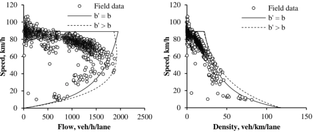
vehi-cles during very low volume conditions; second, S would be set to the inverse of jam density (measured, for example, from aerial photos) and, finally, the reaction time τ would be manually adjusted to make the curvature of the theoretical curve fit the ob-servations. However, as illustrated in Figure 1 (case b = b’), applying this procedure to real detector data usually results in a good fit in the congested regime and a sub-optimal fit in the uncongested regime. This is because the steady-state solution of Gipps’ model predicts constant speed in the uncongested branch and, for b = b’, capacity at the free-flow speed. However, numerous field studies show that speed is sensitive to free-flow and speed-at-capacity is lower than free-flow speed. Punzo and Tripodi [6] noted that the fit can be improved by adopting a value b’ > b. In fact, this relation increases the cur-vature of the congested branch and results in a speed-at-capacity lower than free-flow speed (Figure 1, case b‘ > b). Punzo and Tripodi (op. cit.) also suggested that, to be suitable for real applications, steady-state relationships must be generalized to multi-class traffic flows and they proposed an analytical solution for two vehicle multi-classes. De-spite being a promising approach, the resulting formulation was also unable to predict speed variation in the uncongested branch of the q-v relationship.

Surprisingly, the solution to this problem had been indicated earlier by Gipps [7]. Remembering that the deduction of the steady-state relationships was based on the as-sumption of uniform flow, Gipps found that the distribution of desired speeds affects the shape of the uncongested branch. That is, the final steady-state behavior should be seen as the interaction of the average steady-state parameters with the effect of varia-bility. Following this lead, Farzaneh and Rakha [8] investigated the effect of desired speed variability on the INTEGRATION micro-simulator, based on the Van Aerde steady-state relationship [9], and concluded that model users can control the curvature of the uncongested steady-state behavior to a limited extend by adjusting the coefficient of variation of the desired speed distribution. According to Lipshtat [10], this is because of two opposing effects: on one hand, higher variability in the speeds means more

oc-casions when faster vehicles are delayed by slower ones; on the other hand, more vari-ability also leads to greater distances between successive vehicles, making lane chang-ing easier.

Fig. 1. Adjustment of the q-v and q-k relationships to field data (A44 freeway, Portugal): vmax ₌

89 km/h, S = 8.5 m, case 1: b = b’ = 3 m/s2_{, τ = 1.0 s; case 2: b = 3 m/s}2_{, b’ = 3.6m/s}2_{, τ = 0.6 s;}

θ = τ/2.

To investigate the effect of the desired speed variability on the macroscopic relation-ships, we performed a sensitivity analysis in which was assumed that the desired speed of each vehicle released into the network follows a normal distribution with fixed co-efficient of variation (CV = 10%) for three different average values (vmax= 50, 70 and 90 km/h). The remaining values were set as follows: τ = 0.75 s, θ = τ/2 (hard-coded in Aimsun), S = 5 m, b = 4 m/s2_{, b’ = 4 m/s}2 _{(see Figure 2). It becomes clear that the} adoption of a lower desired speed leads to a lower capacity and that variability in the desired speeds leads to a q-v diagram in which speeds decrease with flow in the uncon-gested branch, thus leading to a capacity reduction and speed-at-capacity lower than free-flow speed, as observed in the real world. Therefore, it seems reasonable to express the expected simulation macroscopic relationships as functions of the parameters vmax_, τ, S and also CV (coefficient of variation of the desired speed).

0 20 40 60 80 100 120 0 500 1000 1500 2000 2500 S p ee d , k m /h Flow, veh/h/lane Field data b' = b b' > b 0 20 40 60 80 100 120 0 50 100 150 S p ee d , k m /h Density, veh/km/lane Field data b' = b b' > b 90 km/h 70 km/h 50 km/h 0 20 40 60 80 100 0 1000 2000 3000 v (k m/ h ) q (veh/(h.lane)) CV = 10%

Fig. 2. Sensitivity analysis of the Gipps steady-state parameters

The introduction of the CV allows the simplification b = b’ and the consequent elim-ination of these two parameters from the calibration process. The problem of this ap-proach is that the effect of variability in the desired speeds is the result of random in-teractions between vehicles which may depend on several factors such as the road ge-ometry, driver and vehicle characteristics. In order to make this calibration approach simulation free, the following section describes the construction of a look-up table that enables the shape of the q-v and k-v curves for a given CV to be analytically identified.

2.3 Derivation of a Look-up Table to Describe the Uncongested Regime

The first step towards the construction of the look-up table was to decide on the shape of the q-v curve in the uncongested regime. This question was previously addressed by Wu [11], who proposed a macroscopic model in which the equilibrium speed-flow-density relationships are described as a superposition of homogeneous states. Specifi-cally, in the uncongested part of the diagram (fluid traffic) Wu’s model considers two possible states: vehicles moving freely at their desired speed (free state) or bunched vehicles traveling in succession (convoy state, or fluid platoon). Assuming pure sta-tionary conditions and equal distribution of traffic in all lanes, the speed in the uncon-gested regime can be expressed as a function of the density k, the free-flow speed vmax_,

the number of lanes N, the speed vko and density kko within the platoons:





1 max max ( ) for N ko ko ko k v k v v v k k k            (5)

This indicates that the k-v relationship is linear in a two-lane road (one-way), quadratic in a three-lane road and so on. The case N = 1 is especially interesting: according to this formulation, the speed on the road is vko regardless of the density, that is, all vehicles

are in platoons. Naturally, this only happens under pure stationary conditions. On real world roads, fast vehicles travel in platoons only for a limited stretch of the road.

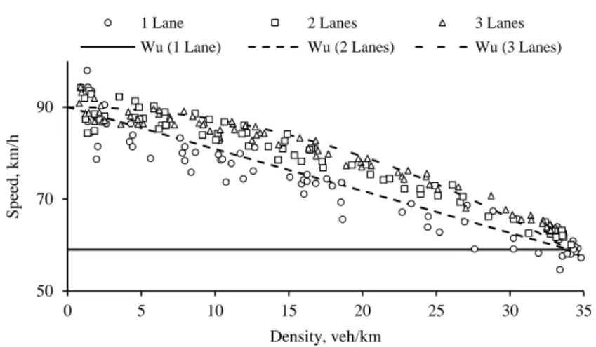
In order to better understand how simulation results agree with Wu’s formulation, k-v measurements were obtained at the middle section of a 1000 m link, for different demand levels and numbers of lanes (vmax _{= 90 km/h, CV = 0.15, N}_{{1, 2,3}). The}

resulting capacity parameters were kC = 34 veh/(km·lane) and vC = 59 km/h. When

these parameters are used in (5) we conclude that the one-lane model must be rejected, as it underestimates speeds at all densities below kC, the two-lane model (linear)

pro-vides a good-fit for 1-lane and 2-lane roads, while the 3-lane model (quadratic), is a good fit with the simulation results on 2-lane and 3-lane roads.

Taking Wu’s linear model for the k-v relationship (which is reasonable for up to three lanes), we can obtain the capacity parameters as the intersection of the uncon-gested and conuncon-gested branches.

Fig. 3. Density-Speed relationships in the uncongested regime: Wu's model (lines) vs simulation

results (markers)

For the uncongested branch – linear model with intercept vmax _{and slope b:}

max

vv k b. At the congested branch – resulting from Gipps’ spacing-speed equa-tion: v 



1 kS

 

/ 1.5k



. The intersection of the two curves occurs for:





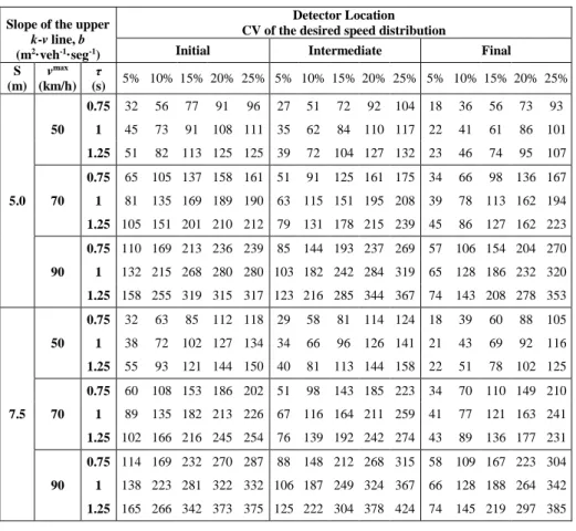
2 max max 3 2 3 2 24 6 C v S v S b k k b           (6)

Finally, the slope of the k-v relationship was obtained from a full factorial experi-ment involving the following simulation parameters: Number of lanes: 2; Section lengths: 500 m, 1000 m and 1500 m; Measurement locations: every 50 m; Effective vehicle lengths: 5, 7.5 and 10 m; Reaction times τ: 0.50, 0.75, 1.00 and 1.25 s; Mean desired speeds vmax_{: 50, 70, 90 and 120 km/h; Coefficients of variation: 5%, 10%, 15%,}

20%, 25% and 30%. For each combination of parameters a very high demand was set at the input centroid, thus assuring the observation of capacity conditions; the simula-tion was allowed to run for 30 minutes. Speed and flow measurements were obtained at each detector at the end of each 5 minute period. Capacity parameters were calculated as the average of the last five measurements, but the first period was excluded, in order to assure stable flow. The analysis of the results made it possible to conclude that the section length has less effect on the slope than the other parameters and that the meas-urement locations could thus be clustered in three regions: initial (first third), middle (second third) and final (last third). The experimental conditions dictate that the result-ing look-up table (Table 1) is roughly discretized, requirresult-ing crossed interpolation to find the slope b for specific cases outside the discrete domain.

50 70 90 0 5 10 15 20 25 30 35 S p ee d , k m/ h Density, veh/km

1 Lane 2 Lanes 3 Lanes Wu (1 Lane) Wu (2 Lanes) Wu (3 Lanes)

Table 1. Look-up table for the slope of the k-v relationship (partial view)

Slope of the upper k-v line, b (m2_·veh-1_·seg-1₎

Detector Location CV of the desired speed distribution

Initial Intermediate Final

S (m) vmax (km/h) τ (s) 5% 10% 15% 20% 25% 5% 10% 15% 20% 25% 5% 10% 15% 20% 25% 5.0 50 0.75 32 56 77 91 96 27 51 72 92 104 18 36 56 73 93 1 45 73 91 108 111 35 62 84 110 117 22 41 61 86 101 1.25 51 82 113 125 125 39 72 104 127 132 23 46 74 95 107 70 0.75 65 105 137 158 161 51 91 125 161 175 34 66 98 136 167 1 81 135 169 189 190 63 115 151 195 208 39 78 113 162 194 1.25 105 151 201 210 212 79 131 178 215 239 45 86 127 162 223 90 0.75 110 169 213 236 239 85 144 193 237 269 57 106 154 204 270 1 132 215 268 280 280 103 182 242 284 319 65 128 186 232 320 1.25 158 255 319 315 317 123 216 285 344 367 74 143 208 278 353 7.5 50 0.75 32 63 85 112 118 29 58 81 114 124 18 39 60 88 105 1 38 72 102 127 134 34 66 96 126 141 21 43 69 92 116 1.25 55 93 121 144 150 40 81 113 144 158 22 51 78 102 125 70 0.75 60 108 153 186 202 51 98 143 185 223 34 70 110 149 210 1 89 135 182 213 226 67 116 164 211 259 41 77 121 163 241 1.25 102 166 216 245 254 76 139 192 242 274 43 89 136 177 231 90 0.75 114 169 232 270 287 88 148 212 268 315 58 109 167 223 304 1 138 223 281 322 332 106 187 249 324 367 66 128 188 264 342 1.25 165 266 342 373 375 125 222 304 378 424 74 145 219 297 385

3

Application

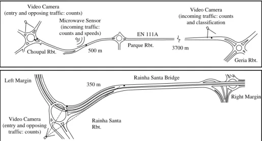
Two sites in Coimbra, Portugal, were selected to illustrate the calibration procedure (see Figure 4). The first is a 4.2 km section of the EN-111A road, between the Geria and Choupal roundabouts. This road is one of the main entries to the city center, used mostly by passenger vehicles. It only has one lane in each direction and gets congested during the morning rush hour. The second site, included for verification purposes, is an off-ramp of the Rainha Santa Bridge, in the W-E direction (350 m), which connects to a single-lane roundabout with intense opposing traffic.

Given the objectives of this study, every effort was made to prevent the introduction of measurement errors, particularly ones related to traffic generation. A video camera was installed near the Geria Rbt to record the type and passage times of approaching vehicles under free-flow conditions. A second camera was placed at the Choupal Rbt to record the passage times of entry and opposing vehicles and, finally, a microwave Doppler detector was installed between the Parque and Choupal roundabouts to collect macroscopic data on approaching vehicles (one-minute average speeds and flows).

Travel times were measured at 5-minute intervals by recording the times at which se-lected vehicles passed the Geria and Choupal roundabouts. There were some minor differences in the counts for each of these periods, but these were corrected by assuming a corresponding number of U-turns at the Parque Rbt, according to an exponential dis-tribution. A video camera was installed at a high point at the Rainha Santa Bridge to simultaneously record the passage times of the entry and opposing traffic. This data was used to generate vehicles with a one-second precision in the simulator, overriding the default generation algorithm.

Fig. 4. Layout of application sites

Two sets of parameters were considered for the calibration process: the first set is di-rectly related to the car-following behavior (the reaction time τ, the desired inter-vehicle spacing at stop s and the average and standard deviation values of the speed acceptance factor (μsa, σsa), which relates the free flow speed vmax with the posted speed); the second

set is mostly related to interrupted flow and driver behavior at intersections (maximum acceleration a, normal deceleration b, reaction time at stop RTS and maximum give way time GWT). RTS is the time it takes for a stopped vehicle to react to the acceleration of the vehicle in front, GWT is used to determine when a driver starts to get impatient if he/she cannot find a gap. With the exception of the abovementioned speed acceptance factor, the vehicles were assumed to be identical.

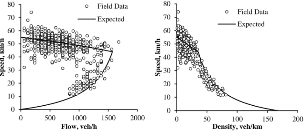
The first part in the calibration process was to fit the macroscopic relations to the speed-flow data collected with the microwave sensor (Figure 5). After a few manual attempts, the parameters S = 6.0 m (s = 2.0 m, L = 4.0 m) and τ = 1.20 s were identified as those providing the best adjustment of the lower branch of the q-v curve (4) to the field data (specifically, to the lower side of the point cloud, to minimize the effect of driver het-erogeneity). In order to plot the upper branch, the free flow speed (average – 54.2 km/h, standard deviation – 9.2 km/h, coefficient of variation – 17%) was directly measured from field data during periods of very low traffic (q < 120 veh/h). The relation between the free-flow speed and posted speed (μsa = 54.2/50 = 1.08) was assumed constant and

Video Camera (incoming traffic: counts

and classification Video Camera

(entry and opposing traffic: counts) Microwave Sensor

(incoming traffic: counts and speeds)

3700 m 500 m EN 111A Parque Rbt. Choupal Rbt. Geria Rbt. Video Camera (entry and opposing

traffic: counts)

Rainha Santa Bridge 350 m

Rainha Santa Rbt.

Right Margin Left Margin

used to estimate the free flow speed at the upstream section, where the posted speed is 90 km/h. Finally, an approximation for the v-k slope was obtained from the look-up table (slope b ≈ 85). The resulting curve (Figure 5) for the uncongested branch follows the field data satisfactorily, thus validating the choice of parameters. The intersection with the lower branch – Eq. (6) yields the capacity parameters: vc = 43.1 km/h, kc = 36.3

veh/km, qc =1565 veh/h. The second part addressed the parameters a, b, RTS and GWT.

As none of these parameters is involved in the steady-state relationships or can be easily measured from field observations, the calibration takes the form of an optimization problem. In this application a procedure based on a genetic algorithm (GA) was fol-lowed. This is a widely used technique that utilizes ideas from natural evolution to ef-fectively find good solutions for combinational parametric optimization problems. The parameter calibration problem was formulated in the following optimization framework [1]: minimize f a b RTS GWT_{, , ,}



Mobs,Msim



subject to the constraints 2 ≤ a ≤ 6 m/s

2_{, 2 ≤ b} ≤ 6 m/s2_{, 0.5 ≤ RTS ≤ 3.0 s with RTS ≥ τ and 0 ≤ GWT ≤ 30 s ,where f is the goodness} of fit function that measures the distance between the observed and simulated measure-ments, obs

M and sim

M .

Fig. 5. Field observations and expected Speed-Flow and Density-Flow relationships at EN111A,

between Parque and Choupal roundabouts

We were particularly interested in understanding how Aimsun was able to predict the variation of queue lengths during the simulation period and so the vector M was defined as the vehicle density between the Geria and Choupal roundabouts at each 1-minute observation/simulation period i. To measure the goodness of fit, the GEH statistic was preferred to other more commonly used measures such as the root mean square error due to its self-scaling property, which allows the use of a single acceptance threshold when comparing a wide range of traffic volumes. Its definition is:





1 2 1 N obs sim i i obs sim i i i M M MGEH N  M M   



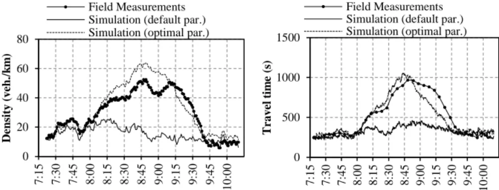
. (7) 0 10 20 30 40 50 60 70 80 0 500 1000 1500 2000 S p ee d , k m /h Flow, veh/h Field Data Expected 0 10 20 30 40 50 60 70 80 0 50 100 150 200 S p ee d , k m /h Density, veh/km Field Data Expected

The optimization framework was implemented in Matlab using the built-in genetic algorithm tool. The algorithm starts by generating an initial population (100 individu-als, each of which corresponds to a set of 4 parameters). For each individual, a Python script modifies the corresponding parameters in Aimsun, simulates the model in con-sole mode and compares the observation and simulation outputs to compute the fitness value. When all individuals are evaluated, the GA generates a new population: besides elite children, who correspond to the individuals in the current generation with the best fitness values, the algorithm creates crossover children by selecting vector entries from a pair of individuals, and mutation children, by applying random changes to a single individual [12]. After 74 generations and approximately 3.5 hours of computing time, the algorithm reached a convergence condition and returned the optimal solution: a = 5.95 m/s2_{, b = 3.78 m/s}2_{, RTS = 1.29 s and GWT = 1.35 s. The field and simulation} measurements of the density and travel times are presented in Figure 6, left and right panels, respectively. Despite a slight overestimation of the maximum values, the simu-lation with optimized parameters generates a satisfactory fit to the field data, particu-larly in comparison with the simulation using the default parameters. It is also relevant to note the robustness of the estimation: similar results were obtained for both variables, even though only density was explicitly evaluated by the fitness function.

Fig. 6. Time-series of Density and Travel Time at the first site (EN-111A): field observations vs

simulation outputs

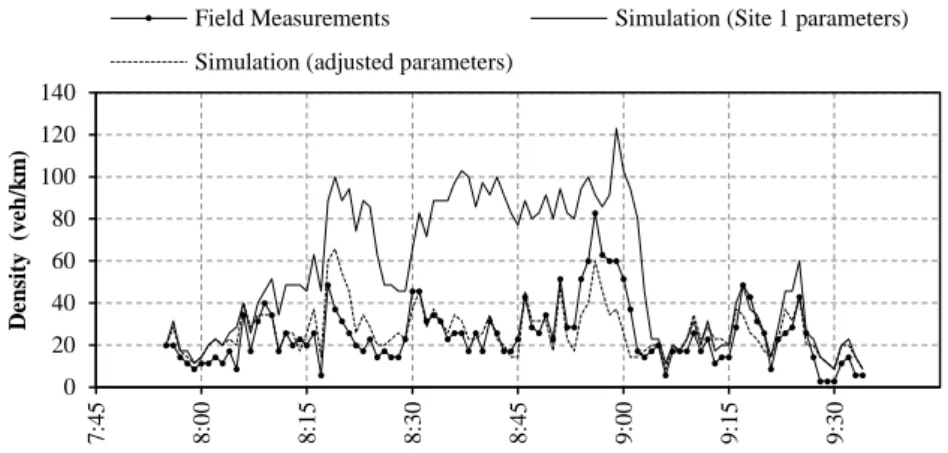
Finally, we looked at how the results of this calibration can be used in a different loca-tion. The traffic at the second site – Rainha Santa Brige – has a vehicle mix similar to EN-111A, so the corresponding full set of optimized parameters was used for the first attempt (see Figure 7). The model overestimated the density in the peak period, indi-cating lack of capacity at the downstream roundabout. A visual inspection of the simu-lation revealed excessively cautious maneuvers at the roundabout entry. This was not a key issue at the first site because the opposing traffic was very light, making the model relatively insensitive to the parameters affecting the entry maneuvers. A few manual adjustments were thus made to improve the gap-acceptance behavior: τ was reduced to 0.95 s and RTS was updated by assuming the same relation between these parameters; the maximum give way time GWT was set to a very low value, thus reducing the waiting

0 20 40 60 80 7 :1 5 7 :3 0 7 :4 5 8 :0 0 8 :1 5 8 :3 0 8 :4 5 9 :0 0 9 :1 5 9 :3 0 9 :4 5 1 0 :0 0 D en si ty ( v eh ./ k m ) Field Measurements Simulation (default par.) Simulation (optimal par.)

0 500 1000 1500 7 :1 5 7 :3 0 7 :4 5 8 :0 0 8 :1 5 8 :3 0 8 :4 5 9 :0 0 9 :1 5 9 :3 0 9 :4 5 1 0 :0 0 T ra v el t im e (s) Field Measurements Simulation (default par.) Simulation (optimal par.)

time at the yield line. The simulation with the adjusted parameters now closely follows the field density time-series. These results suggest that the macroscopic estimation pro-cedure yields relatively robust parameters, that is, they can be applied to different loca-tions with satisfactory results, provided that the traffic has a similar composition at both locations. The traditional methods, however, being based on “blind” optimization, dis-regard the parameters’ physical meaning and can lead to biased estimates that reduce the explanatory power of the model.

Fig. 7. Time-series of Density at the second site (Rainha Santa Bridge): field observations vs

simulation outputs

4

Conclusions

Current macroscopic calibration procedures for the Gipps car-following model assume constant speeds in the uncongested regime, whereas numerous field studies indicate that the speed-flow diagram is curved in both the congested and uncongested regimes. In this paper we have shown that it is essential to account for the variability in the drivers’ desired speed distribution to accurately reproduce the uncongested part of the field speed-flow data. We used a vast set of simulations to construct a look-up table that relates the slope of the density-flow relationship with the vehicles’ desired speed variability and with other variables that also have a significant effect in the macroscopic relationships, such as the detector location and the vehicles’ effective length and reac-tion time. This procedure was used in a real-world calibrareac-tion problem, as part of a broader calibration framework that also includes a conventional optimization based on a genetic algorithm. The car-following parameters resulting from the macroscopic cal-ibration proved to be robust, which enabled their use at different locations with only minor adjustments, and showed that the new methodology is promising in terms of practical applicability. 0 20 40 60 80 100 120 140 7 :4 5 8 :0 0 8 :1 5 8 :3 0 8 :4 5 9 :0 0 9 :1 5 9 :3 0 D en si ty (v eh /k m )

Field Measurements Simulation (Site 1 parameters) Simulation (adjusted parameters)

Acknowledgements. This work was supported by FCT (Portugal) under the R&D

project PTDC/SEN-TRA/122114/2010 (AROUND – Improving Capacity and Emis-sion Models of Roundabouts).

References

1. Ciuffo, B., V. Punzo, and V. Torrieri, Comparison of Simulation-Based and

Model-Based Calibrations of Traffic-Flow Microsimulation Models. Transportation Research

Record: Journal of the Transportation Research Board, 2008. 2088(-1): p. 36-44.

2. Punzo, V. and B. Ciuffo, How Parameters of Microscopic Traffic Flow Models Relate

to Traffic Dynamics in Simulation. Transportation Research Record: Journal of the

Transportation Research Board, 2009. 2124(-1): p. 249-256.

3. Casas, J., et al., Traffic Simulation with Aimsun, in Fundamentals of Traffic Simulation, J. Barceló, Editor 2010, Springer New York. p. 173-232.

4. Wilson, E., An Analyses of Gipps' Car-Following Model of Highway Traffic. IMA Journal on Applied Mathematics, 2001. Volume 66(5): p. 509-537.

5. Rakha, H. and W. Wang, Procedure for Calibrating the Gipps Car-following Model, in TRB 2009 Annual Meeting2009, Transportation Research Board: Washington DC. 6. Punzo, V. and A. Tripodi, Steady-State Solutions and Multiclass Calibration of Gipps

Microscopic Traffic Flow Model. Transportation Research Record: Journal of the

Transportation Research Board, 2007. 1999(-1): p. 104-114.

7. Gipps, P.G., A behavioural car-following model for computer simulation. Transportation Research - B, 1981. 15(B): p. 105-111.

8. Farzaneh, M. and H. Rakha, Impact of Differences in Driver-Desired Speed on

Steady-State Traffic Stream Behavior. Transportation Research Record: Journal of the Transportation

Research Board, 2006. 1965(-1): p. 142-151.

9. Rakha, H. and B. Crowther, Comparison of Greenshields, Pipes, and Van Aerde

Car-Following and Traffic Stream Models. Transportation Research Record: Journal of the

Transportation Research Board, 2002. 1802(1): p. 248-262.

10. Lipshtat, A., Effect of desired speed variability on highway traffic flow. Physical Review E, 2009. 79(6): p. 066110.

11. Wu, N., A new approach for modeling of Fundamental Diagrams. Transportation Research Part A: Policy and Practice, 2002. 36(10): p. 867-884.

12. MathWorks, I., Genetic Algorithm and Direct Search Toolbox for Use with MATLAB®: User's Guide2005: MathWorks.