Adaptive algorithms for cost-efficient pump control in water distribution network

(1)

Universidade de Aveiro Ano 2019

Departamento de Engenharia Mecânica

Marcelo Rafael

Sousa Manteigas

Adaptive Algorithms for Cost-Efficient Pump

Control in Water Distribution Network

Algoritmos Adaptativos para Controlo Eficiente de

Bombas numa Rede de Distribuição de Água

(2)

(3)

Universidade de Aveiro Ano 2019

Departamento de Engenharia Mecânica

Marcelo Rafael

Sousa Manteigas

Adaptive Algorithms for Cost-Efficient Pump

Control in Water Distribution Network

Algoritmos Adaptativos para Controlo Eficiente de

Bombas numa Rede de Distribuição de Água

Dissertação apresentada à Universidade de Aveiro para cumprimento dos requisitos necessários à obtenção do grau de Mestre em Engenharia Mecânica, realizada sob a orientação científica de António Gil d’Orey de Andrade Campos, Professor Auxiliar do Departamento de Engenharia Mecânica da Universidade de Aveiro.

Esta dissertação teve o apoio dos projetos UID/EMS/00481/2019-FCT - FCT - Fundação para a Ciência e a Tecnologia; e CENTRO-01-0145-FEDER-022083 - Programa Operacional Regional do Centro (Centro2020), através do Portugal 2020 e do Fundo Europeu de Desenvolvimento Regional.

(4)

(5)

Dedico este trabalho ao meu querido pai, Carlos Alberto Sá Manteigas, sem o qual esta aventura universitária maravilhosa não teria sido possivel.

(6)

(7)

o júri / the jury

Presidente / president Prof. Doutor João Alexandre Dias de Oliveira

Professor Auxiliar Departamento de Engenharia Mecânicada Universidade de Aveiro

Doutor Bruno Alexandre Abreu da Silva Director Executivo, Scubic

Prof. Doutor Gil D’Orey de Andrade Campos

Professor Auxiliar Departamento de Engenharia Mecânicada Universidade de Aveiro (orientador)

(8)

(9)

agradecimentos _{Ao meu pai pelo incansável apoio em todos os meus desafios e} conquistas.

Ao meu orientador por inspirar a exigência que uma dissertação merece, e pelas discussões abertas que originaram muitas das ideias aplicadas neste trabalho.

Aos meus grandes amigos, João Veloso, João Marques e Gonçalo Silva, por me acompanharem nestre processo assim como em toda a minha aventura universitária.

Aos meus colegas do projecto Learning Experiment, por me motivarem a aprender mais e a continuar curioso.

À minha namorda, Eniko Kosztolanczi, por me incentivar a cumprir as minhas responsabilidades académicas em vez de apreciar um belo jantar de sushi, e uma caminhada à beira mar. À Universidade de Aveiro por proporcionar um ecosistema rico e dinâmico para aprender e crescer.

Por fim, obrigado a todas as pessoas que fizeram parte do meu caminho e sem as quais não seria o ser humano que sou hoje!

(10)

(11)

palavras-chave Algoritmos Adaptativos, Estratégia de Bombeamento, Eficiência, Rede de Distribuição de Água, Modelos de Controlo, Controlo Adaptativo.

resumo Cidades modernas têm redes de distribuição de água que de forma confiável satisfazem as necessidades de água de todos os domicílios. Estas redes dependem de bombas para mover a água de fontes distantes ao consumidor. Se gerido de forma ineficiente, este processo consumidor de energia pode tornar-se muito dispendioso. Através de poder computacional emergente, tecnologias de simulação e sensores, muitas técnicas foram desenvolvidas para produzir as melhores estratégias de operação. Estas metodologias dependem de previsões do consumo de água para criar estratégias de bombeamento óptimas. Porém, estas previsões contêm sempre erros, que podem criar problemas de controlo. Muitos esforços foram feitos para desenvolver melhores previsões, algumas das quais podem mudar os seus parâmetros em tempo real. De qualquer forma, estas soluções ainda contem erros e não conseguem adaptar a mudanças drásticas de consumo. Para resolver este problema é proposto um controlo adaptativo capaz de eficientemente actualizar em tempo real a estratégia de bombeamento com base nos desvios monitorizados relativamente à previsão. Esta metodologia toma em consideração uma referência optimizada para continuamente fazer as actualizações mais eficientes à estratégia de bombeamento. Para validar o controlo adaptativo, dois casos de estudo foram explorados: (i) uma rede simples composta de uma bomba e um tanque, (ii) e a de rede de referência de Richmond. Ambas as avaliações entregaram resultados positivos melhorando a eficiência a nível de custo. A combinação de previsões de consumo de água com metodologias de controlo adaptativo providencia uma solução confiável e eficiente para controlo automático de redes de distribuição de água. Este modelo de controlo pode se tornar uma característica essencial na tecnologia emergente “water grids” fechando o ciclo de controlo no sistema. .

(12)

(13)

keywords Adaptive Algorithm, Pumping Strategy, Cost-Efficiency, Water Distribution Network, Control Model, Adaptive Controller.

abstract Modern cities have water distribution networks (WDN) that reliably meet the water demand of every individual household. These networks rely on pumps to move water from distant sources to the consumer. If inefficiently managed, this energy consuming process can become very costly. Using emerging computer power, simulation technologies and sensing devices, many techniques were developed that produce the most cost-efficient operational strategies. These methodologies rely on water consumption predictions to provide optimal pumping strategies. However, these predictions always contain errors, which may create control problems. Many efforts were made to develop progressively better predictions, some of which can change its parameters in real time. Nevertheless, these solutions still contain errors and cannot adapt appropriately to sudden changes in demand. To solve this problem, an adaptive controller that can efficiently update the pumping strategy based on monitored deviations of the predicted consumption is proposed. This methodology takes into account the tariffs of electricity over time and an optimal reference to continuously make the most cost-efficient updates in the pumping strategy. To validate the adaptive controller, two case studies were used: (i) a simple pump-reservoir network and (ii) the Richmond benchmark network. Both evaluations delivered positive results achieving the desired reliability while improving cost efficiency. The combination water consumption predictions and adaptive control methodologies provide a reliable and cost-efficient solution to operate a WDN automatically. This control model may become an essential feature in emerging water grids technology by closing the loop in the control system.

(14)

(15)

i

List of Figures

Fig.1 – Main sectors of a water supply system from the source to the end user

[9]. ... 2

Fig. 2 – Smart water grids technology scheme [8] ... 4

Fig. 3 – Smart water network typical layout [7]. ... 5

Fig. 4 – Scheme describing the optimal operation of WDN using a SCADA system [9]. ... 6

Fig. 5 – Dynamic Real-time Adaptive Genetic Algorithm – Artificial Neural Network [6]. ... 7

Fig. 6 – Adaptive LQR control model for pumping stations [16]... 9

Fig. 7 – Adaptive control architecture. ... 14

Fig. 8 – Flow sequence of the adaptive controller. ... 15

Fig. 9 – Best pumping options at the control increment 𝑘 = 0 for negative disturbance. ... 18

Fig. 10 – Best pumping options at control increment 𝑘 = 0 for positive disturbance ... 19

Fig. 11 – Flow diagram of the decision-making algorithm. ... 24

Fig. 12 – Subsystem F network scheme [26]. ... 28

Fig. 13 – Richmond network scheme [11]. ... 29

Fig. 14 – Average water consumption bias for the subsystem F network, test 1. ... 33

Fig.15 - Water consumption for over biased deviation in subsystem F, test2 ... 33

Fig. 16 - Water consumption for over biased deviation in Richmond network, test 2. ... 34

Fig. 17 - Water consumption for lower biased deviation for the subsystem F, test 3. ... 34

Fig. 18 - Water consumption for lower biased deviation for the Richmond network, test 3. ... 35

Fig. 19 - Water consumption for noisy averaged biased deviation for the subsystem F, test 4. ... 35

Fig. 20 - Water consumption for noisy averaged biased deviation for the Richmond network, test 4. ... 36

Fig. 21 - Water consumption for higher over biased deviation in subsystem F, test 5. ... 36

Fig. 22 - Water consumption for fire situation with average biased deviation in subsystem F, test 6. ... 37

Fig. 23 - Water consumption for fire situation with average biased deviation in Richmond network, test 6. ... 37

Fig. 24 - Water consumption for average biased deviation with missing data for the subsystem F, test 7. ... 38

(18)

iv

Fig. 25 – Linear relation between pumping time and water level of the tank for subsystem F ... 39 Fig. 26 – Results for average consumption bias test: (a) chart that represent the

reliability success of each controller, (b) chart that represent the average cost for each control method, (c) Water level of the tank for each control method, (d) Pumping strategy for each control method. ... 45 Fig. 27 – Results for overconsumption bias test: (a) chart that represent the

reliability success of each controller, (b) chart that represent the average cost for each control method, (c) Water level of the tank for each control method, (d) Pumping strategy for each control method. ... 46 Fig. 28 – Results for underconsumption bias test: (a) chart that represent the

reliability success of each controller, (b) chart that represent the average cost for each control method, (c) Water level of the tank for each control method, (d) Pumping strategy for each control method. ... 47 Fig. 29 – Results for noisy average consumption bias test: (a) chart that

represent the reliability success of each controller, (b) chart that represent the average cost for each control method, (c) Water level of the tank for each control method, (d) Pumping strategy for each control method. ... 48 Fig. 30 – Results for higher overconsumption bias test: (a) chart that represent

the reliability success of each controller, (b) chart that represent the average cost for each control method, (c) Water level of the tank for each control method, (d) Pumping strategy for each control method. ... 49 Fig. 31 – Results for Fire situation with average consumption bias test: (a) chart

that represent the reliability success of each controller, (b) chart that represent the average cost for each control method, (c) Water level of the tank for each control method, (d) Pumping strategy for each control

method. ... 50 Fig. 32 – Results for missing data situation with average consumption bias test:

(a) chart that represent the reliability success of each controller, (b) chart that represent the average cost for each control method, (c) Water level of the tank for each control method, (d) Pumping strategy for each control method. ... 51 Fig. 33 – Forecasted water level of the tanks for the Richmond network. ... 54 Fig. 34 – Results for fire situation test: (a) the water level of every tank of the

Richmond network with the reference control strategy and, (b) with the adaptive control strategy. ... 55 Fig. 35 – Results for average consumption with noise test: (a) the water level of

every tank of the Richmond network with the reference control strategy and, (b) with the adaptive control strategy. ... 56 Fig. 36 – Results for overconsumption test: (a) the water level of every tank of

the Richmond network with the reference control strategy and, (b) with the adaptive control strategy. ... 57

(19)

v

Fig. 37 – Results for underconsumption test: (a) the water level of every tank of the Richmond network with the reference control strategy and, (b) with the adaptive control strategy. ... 58

(20)

(21)

vii

List of Tables

Table 1 – Price tariff over the day. ... 16 Table 2 – Type of test performed to evaluate the performance of the adaptive

controller ... 32 Table 3 – Constraints for the tanks of the Richmond network ... 38 Table 4 – Constant Pump-Tank relations for the Richmond network ... 40 Table 5 – Cost of operation for all tests performed for each control method .... 59

(22)

(23)

ix

Nomenclature

Symbol Description Unit

𝑑 Disturbance. [m]

𝑘 Control increment. [-]

𝑦opt𝑘 Forecasted water level of

the tank at control increment𝑘.

[m]

𝑦𝑘 Measured water level of

the tank at control increment𝑘.

[m]

x_opt𝑘,…,𝑛𝐼𝑛𝑐 = [𝑥_opt0 , … , 𝑥_opt𝑘 , … , 𝑥_opt𝑛𝐼𝑛𝑐] Initial optimal pumping strategy.

[min] or [%] y_opt𝑘,…,𝑛𝐼𝑛𝑐 = [𝑦opt0 , … , 𝑦opt𝑘 , … , 𝑦opt𝑛𝐼𝑛𝑐] Initial forecast of the water

level of the tank over the whole control period.

[m]

𝑥𝑘 Pumping time at control

increment𝑘. [min] or [%] 𝑛𝐼𝑛𝑐 Number of control increments in a 24 h control period. [-] x𝑘;𝑘,…,𝑛𝐼𝑛𝑐_{= [} 𝑥 0;0_𝑥𝑘;0_𝑥𝑛𝐼𝑛𝑐;0 − − − 𝑥𝑘;𝑘 𝑥𝑛𝐼𝑛𝑐;𝑘 − − − − − − 𝑥𝑛𝐼𝑛𝑐;𝑛𝐼𝑛𝑐 ]

Pumping strategy at𝑘. [min] or [%]

x𝑘+1;𝑘,…,𝑛𝐼𝑛𝑐 New pumping strategy at

𝑘 + 1. [min] or [%] y_est𝑘;𝑘,…,𝑛𝐼𝑛𝑐 = [ 𝑦0;0 𝑦𝑘;0 𝑦𝑛𝐼𝑛𝑐;0 − − − 𝑦𝑘;𝑘 𝑦𝑛𝐼𝑛𝑐;𝑘 − − − − − − 𝑦𝑛𝐼𝑛𝑐;𝑛𝐼𝑛𝑐 ]

Estimation of the water level of the tank for the whole control period at𝑘.

[m]

y_est𝑘+1;𝑘,…,𝑛𝐼𝑛𝑐 Estimation of the water

level of the tank for the whole control period at𝑘.

[m]

𝑖 Adaptation option. [-]

𝑙 Number of adaptation

options.

(24)

x

t_p Array with the price levels

of each control increment

𝑘.

[-]

p_h𝑘;𝑖,…,𝑙 Hierarchy control update

vector at control increment

𝑘.

[-]

∆𝑦 Variation of water level of

the tank.

[m]

∆𝑥 Amount of pumping time

that increases or

decreases the water level by∆𝑦 .

[min] or [%]

𝑚 Constant relating the

amount of pumping time with the amount of water level in the tank.

[m/min]

hmin Minimum water level of the

tank.

[m]

h_max Maximum water level of the

tank.

[m]

𝐤_𝑣𝑘 _{Control increment 𝑘 at}

which the constraints are violated.

[-]

p_hv𝑘;𝑖,…,𝑙 Hierarchy control update

that validates the constraints.

[-]

∆𝑥_correct Amount of pumping time

necessary to correct the disturbance.

[-]

𝑏𝑘 _{Buffer amount at control}

increment 𝑘.

[-]

𝑏0 Initial buffer parameter. [-]

𝐱_adp𝑖 Amount of time to adapt at

adaptation option 𝑖.

[min] or [%]

(25)

1

1 Introduction

“The cornerstone of any healthy civilization is access to safe drinking water.” (Larry W. Mays) “One of the most vital services to industrial growth is an adequate water supply system” (Larry W. Mays) “Water not only feeds bodies, but it also feeds countries.” (SENSUS, 2012)

1.1 Motivation

Water is undeniably one of the most essential elements of life. Historically, civilizations would sprout in the vicinities of vast water reservoirs, such as Mesopotamia. Besides that, ready access to safe drinking is one of the best predictors of life quality and progress [1].

The creation of water distribution networks facilitated the access to places where before it was impossible. This allowed civilization to spread to other areas of the globe [1] and have access to additional resources.

Nowadays, the dependency on water has grown to industrial levels and it’s fundamental for the economy, having influence in every single sector. This is another indication that as society evolves, so does the dependency on water. With the increase in water demand, it also increases the energy demand to operate a WDN. Therefore, it’s paramount to build ever more productive, reliable, and optimal WDN to support civilization constant growth.

“If we dare to dream of a future utopia, we must first work towards a utopic water distribution system” (Marcelo Manteigas 2019)

(26)

2

1.2 Framework

A water distribution network (WDN) is an infrastructure with the primary purpose of moving water from distance sources to the individual consumer in the required quantity and at sufficient pressure [1].

Without a WDN, it’s extremely difficult to populate the most remote areas of the world. It allows cities to spread away from water sources, making it possible to explore other resources. This shows the relevance of the impact a WDN has on modern society. Most modern cities already have robust and reliable infrastructures of WDN. Such infrastructures are composed of several sections, with different purposes.

Figure 1, illustrates the mains sectors of the course of water from its source until the final consumer. Although most of the process is done harnessing the power of gravity, it still is necessary to resort to pumping stations to move the water at adequate pressure, from its abstraction until its destination. Therefore, to effectively operate a WDN, the crucial decision that must be made is which pumps should be operated at any given time, as Walski pointed out [2]. This decision faces 3 very important competing goals: (i) maximize reliability, customers must always have access to water; (ii) minimize energy cost, the supply systems have to meet the demand while efficiently operating the network; (iii) Meet water-quality standards, which involves reducing the time water stays in storage tanks.

Fig.1 – Main sectors of a water supply system from the source to the end user [9].

To operate the pumping stations it is required electrical energy, which means that managing a WDN involves both the responsibility of reliably moving water and managing energy consumption. In fact, the global water supply represents a significant portion of global energy consumption, which equates to about 7% of all energy consumed [3]. Thus, the water sector has increased responsibility for the sustainable use of this planet resources since it handles two of the most important: water and energy.

This poses a massive opportunity for potential solutions since any small tool created to attenuate water waste products generates a significant positive impact on reducing the global expense of moving and managing water. It is also estimated that 30% of water is lost due to water leakages in the WDN, meaning a similar portion of the energy is also lost [4], furthermore, the inefficient operation

(27)

3 of pumps may represent an equal amount of waste. This opportunity is expected to be even higher in the future, as it’s predicted through the population growth trends and industry development. The forecast indicates that the water industry will reach the trillion-dollar mark by 2050 [4]. This is a clear indication of the potential technological advancements that have to be explored, both for economic benefits but also for the sustainability of the planet.

The indicators of high energy consumption are immediate reflectors of energy costs concerning the operation of WDN. If this consumption is not well managed, this can generate dramatically high energy bills for any given institution. Managing energy might mean different things, depending on the industry. In the water industry, given the electricity price fluctuation over time, means that water should be pumped when possible at periods where the price is lowest. To address this opportunity, the field of automation, control, and optimization have been extensively developed in the academic community. Most of the work accomplished in recent years falls under the umbrella of reducing energy cost without compromising the network reliability and water quality. According to Feldman [5], the main improvements in energy efficiency can be obtained with; (1) pumping stations design improvement; (2) systems design improvement; (3) variable speed drives (VSD) installation; (4) efficient operation of pumps and; (5) leakages reduction through pressure modulation.

Although the opportunity is clear and the technology is already here, the uptake of new procedures in practice has been somewhat disappointing with relatively few being applied to realWDN [6]. The resistance in adopting models mentioned before by the water industry is partly because they are generally complex, involving a considerable amount of mathematical sophistication and substantial computational power, that increases with the size of the network [6]. Besides that, the techniques are confined to minimizing energy cost and largely ignore the network performance.

For the better acceptance of the methods by the industry, the solutions must be holistic, reliable, and simple to use. It is vital to develop robust software applying the similar methods with;(a) intuitive and attractive graphics interfaces, (b) easy adaptation to new situations and, maybe the most critical issue, (c) paying specific attention to the network performance and the consumers supply requirements [6].

To address this necessity, an IoT based technological solution named smart water grids has been developed. “A Smart Water Network is the collection of data-driven components helping to operate the data-less physical layer of pipes, pumps, reservoirs, and valves” [7]. Figure 2, shows the typical scheme of smart water grids technology. This technology makes it possible to leverage the

(28)

4

data collected about the network for an improved, streamlined, and efficient operation.

Fig. 2 – Smart water grids technology scheme [8]

A smart water network is composed of five different layers as layout in figure 3; (1) Automation and control tools in the physical layer, for the automatic and remote execution of actions/tasks received by means of real-time communication channels. (2) Measurement and sensing devices, to collect data from the networks (ﬂow, pressure, water quality, etc.); (3) Real-time communication systems, to gather the collected data and/or to send execution actions (e.g., pumps or valves shut-off); (4) Data management software, to efﬁciently, handle the collected data by means of automatic processing; (5) Real-time data analytics and modelling software, to obtain useful insights from the network data, monitor and evaluate the potential impact of possible changes in the network (e.g. patterns detection, predictive analysis of control scenarios, etc.) [9].

To sense and control is implemented a SCADA that manages the real-time operations. This allows online operational adjustments to possible variations in the network, such as sudden fluctuations in demand, contributing to the efficiency improvements of the WDN. A SCADA system is composed of one or more field data interface devices such as reservoir level meters, water flow meters, valve position transmitters, power consumption meters, and pressure

(29)

5 meters. Thereby, the main functions of a SCADA system are; (1) data acquisition, (2) data communication; (3) data presentation and; (4) control [9]. Figure 4 illustrates how it could be implemented a SCADA system for WDN simplistically, in a smart water grids context.

Fig. 3 – Smart water network typical layout [7].

The fundamental goal of this emerging water grids tecnology is to introduce an automatic control in an “intelligent” way that surpasses that of a human operator. Having access to information the network, it’s possible to create hydraulic models that predict water consumptions. With this insight about the network, it’s possible to apply methodologies to calculate optimal operational strategies, like cost efficient pumping strategies. Through combining mathematical modeling with data sensing devices, this technology can highly improve the performance of the network. However, this is only possible when the hydraulic simulators are adequately calibrated and reflect the real operational characteristics of the network.

The smart water grids technology relies on robust mathematical formulations that manage all the data received concerning the network. A lot of work has been developed to create features that improve its performance. As highlighted at the beginning of this section, any small improvement in the management of water has the potential to produce excellent results due to scale effects. Most improvements are based in refining the quality of water consumption predictions. Recently, solutions based on artificial neural networks have also been explored, having succeeded in surpassing the accuracy performance of hydraulic modeling at representing the network. Yet this is only possible when there is access to large amounts of data about the network, which is not the case for the vast majority of WDN [10].

(30)

6

Fig. 4 – Scheme describing the optimal operation of WDN using a SCADA system [9].

As the next section demonstrates, predictions are always accompanied by errors, and sometimes water consumption might unexpectedly deviate from what is expected. These situations can create control problems and reduce the performance of the network. Dealing with these problems is a central argument in developing automatic systems that can operate in closed loop control for WDN. Emerging reliable technology to run WDN’s is of great interest to institutions that provide this service. Thus this work fits in the framework of improving the usability and end result of these technologies by developing tools that address these problems.

(31)

7

1.3 State of the Art

To effectively control a pumping stations, the decisions must be made having in mind that the customer must always have access to water. After assuring the demand is met, the next goal is to perform this task in the most cost-efficient way. Different strategies have been devised to meet this goal, and the most recent are based on water consumption forecasts. These advancements were made possible due to recent technological developments. In most modern water services institutions, some form of hydraulic modeling, followed by predictions of water consumption and optimal pumping strategies are used to assist the operator in making the best decisions [11].

Fig. 5 – Dynamic Real-time Adaptive Genetic Algorithm – Artificial Neural Network [6].

Although this control methodology is very effective at producing the most cost-efficient operational strategy, it requires additional control from an operator to account for unpredictable changes in demand or unexpected errors in the forecasting. In real time operations, the monitored water consumption is often different from the predictions. These types of controllers do not have the ability to adapt to changes and therefore are weak alternatives to implement in closed-loop control systems [12].

Some systems that try to bypass this problem were designed, such as the DRAGA-ANN( Dynamic Real-time Adaptive Genetic Algorithm – Artificial Neural

(32)

8

Network) [6], a fully adaptive forecasting model proposed by Bakker [13] and the PAWN (Parallel Adaptive Weighting model) [14], that to some extent can adapt to changes in the environment by continuously adjusting their forecasts based on new readings of the network. Figure 5 demonstrates the algorithm used by the DRAGA-ANN system to achieve this purpose. These models can make reliable forecasts of the water consumption, which make possible the creation of optimized strategies to operate the pumping stations, however they are not robust to unexpected changes. They are suitable for real-time operations but it’s necessary supervision from the operators.

A solution to this reliability problem is the typical reactive controller. These controllers don’t use any sort of “intelligence” to control network and are often single objective. The simplest one’s work on the basis of keeping the water level within a certain level. This strategy might be very cost inefficient since it doesn’t leverage the knowledge about the network. Instead, it’s continuously reacting to the demand and adapting the state of the pumps accordingly. Although this methodology does not produce the most cost-efficient strategies, it can reliably assure a closed loop control.

A simple PI (proportional–integral)controller was created for the control of a pumping stations of a WDN but seemed to be unsuitable for solving the problem of effective water distribution control canals characterized by significant time-varying dynamical parameters. The PI controller has the best performance only in nominal conditions, which is not the case of a WDN dynamic [15].

A more sophisticated reactive controller is the adaptive controller. Figure 6 shows the scheme of an adaptive controller design proposed by Elbelkacemi [16]. This architecture is composed of a controller that executes the actions, the plant (or the system to be controlled) that receives such instructions and outputs its response, and an adaptive scheme that results from the combination of a parameter estimation and control design that continuously adapts the controller execution strategy. The use of this controller has benefits; it allows a high-performance control of the system and provides fine tuning of the controller when the reaction of the plant is unknown or time-varying. It has the ability to solve through good approximation some nonlinear stochastic control problems, that can’t be simply solved through gain scheduling [17].

(33)

9

Fig. 6 – Adaptive LQR control model for pumping stations [16].

There are many applications that rely on adaptive controllers to extract the best possible control results. In the water industry, this tool has been applied for water quality control, such as the one created and tested by Zhong [18] and KIOS research center [19]. Shengwei Wang also suggested the application of adaptive controllers to operate variable speed drives [20].

An adaptive controller was built to automatically operate a decentralized water distribution network, with more than 20 pumps to provide water into an agriculture field. This controller main objective is to stabilize the water level of the tanks while reducing water waste products. Although it’s designed to reduce the cost of pumping, it didn’t consider the electricity tariff price in its operation. However, the complex mathematical formulation made it impractical to implement this model in larger systems. Besides that, the controller was single objective, only considering the water level of the tank [21]. A similar model for a simple network has also been implemented by Rivas Pérez [22].

Another real-time optimal controller was designed and tested to work on a water supply system of river Basis [23]. The result is a single objective controller, that was tested using 2 different controller designs; (i) the LQR (linear quadratic regulator) and, (ii) MPC (model predictive controller). The controllers had two working frameworks, one dedicated to controlling the water tank level, and the other to control the constant water inflow. Although the results were reasonably good at having a prompt response to disturbance, the control models were not adaptive to the time-varying nonlinear dynamics of a WDN. The model was implemented and tested successfully but was limited to work in open loop. The LQR control algorithm, when combined with an adaptive scheme, has shown better results to control the flow of water, being successful at regularizing the pumping discharges to face the oscillation of demand. However, it doesn’t consider the pumping cost in its control objectives. A similar controller was

(34)

10

designed with a focus on energy efficiency but didn’t take into consideration the electricity price table [24].

There are many adaptive controllers being used to control pumping stations in water distribution networks, although they are successful at dealing with the nonlinear dynamics of WDN, most of them are single objective and mathematically complex, posing a limitation to their application in city-sized WDN, where the solutions must be holistic and straightforward to be implemented [22]. Essentially these are the two state-of-the control methodologies used in pumping stations; one is based on developing extensive insight about the networks that make possible the use of forecasts to leverage the decisions taken by operators. It can work automatically in real-time operations. However, it’s necessary to have some form of supervision from an operator by introducing machine interaction through visual interfaces and alarms to assure the reliability of the systems. The other solution for this concern can reliably control a WDN automatically in closed-loop, by operating on constant feedback with the real monitored readings of the network. The adaptive controllers are more successful with this task. However, the cost of the operation is often not taken into account since the strategies are single cycled, making it less attractive for institutions.

(35)

11

1.4 Objectives

Having studied the literature concerning the control methodologies for the water distribution network, it is clear that the evolution of solutions has diverged into two different realms of thought. One is based on leveraging vast amounts of data to produce the best operational strategies. The other focuses on constant monitoring of the network to make online adjustments to the pumping stations. Although some solutions have tried to integrate both ideas, such as building evolving predictions by monitoring the networks, these are far from perfect and aren’t reliable enough to close the control loop. This means that these methodologies still need user input to run without compromising access to water to the final consumer.

If the objective is to create a functional software feature for the emerging water grids technology to deliver a fully automatic solution to water service providers, an adaptive control methodology might work well, however, due to the lack of consideration over the cost of operation, this solution is not liable to be accepted by the water industry.

There is a clear gap in the literature in experiments that try to develop methodologies that fully merge the advantages of both ideas. Create a controller that can adapt to the environment response, but that also considers the forecasts and knowledge about the network.

The hypothesis is that the solution is to develop a control algorithm that can adapt the previous optimally calculated parameters on the basis of the environment changes. Creating an adaptive controller, that doesn’t adjust to the real consumptions but rather that operates by nullifying the disturbances created by an operating strategy that follows a water consumption forecast.

Thus, the objective of this work is to develop a new methodology to operate the pumping stations that aims at surmounting the current automatic control strategies, and that might become a better fit solution for the emerging water grids technologies.

(36)

(37)

13

2 Methodology

As suggested in the previous section, there is high potential to explore the merging of the two control strategies; (i) control based on forecasts and, (ii) control based on adaptation to continuous measurements of the network state. To accomplish that, the architecture of the controller is similar to the one proposed by Elbelkacemi [16] in figure 6, with a different adaptive algorithm. The adaptive scheme in adaptive controllers uses the online readings of the network to calculate new parameters for the controller. For this project, the adaptive scheme is designed to use these same online readings to nullify the disturbance measured by comparing the real consumptions of the network with the calculated forecast. The disturbance 𝑑 is calculated as;

𝑑 =𝑦opt𝑘 − 𝑦𝑘 , (1)

where 𝑦_opt𝑘 is the predicted water level of the tank at control increment 𝑘 based on the water consumption forecast and optimal pumping strategy x_opt𝑘,…,𝑛𝐼𝑛𝑐, the 𝑦𝑘

is the measured (or real) water level of the tank at the control increment 𝑘. The disturbance 𝑑 is calculated at every control increment 𝑘 and the objective of the adaptive controller is to continuously nullify it in order to allow the cohesion of the initial pumping strategy over time. In a different way of thinking, the disturbance 𝑑 can be seen as an indicator of the accuracy of the forecast, and the purpose of the adaptive controller is to minimize this error in real time. To achieve this purpose, the initial pumping strategy x_opt𝑘,…,𝑛𝐼𝑛𝑐 must be continuously updated.

The adaptation to the measured disturbance 𝑑 is made by intelligently updating the initially introduced pumping strategy x_opt𝑘,…,𝑛𝐼𝑛𝑐, considering the cost efficiency and the reliability of the process. The adaptive scheme seeks for the time periods where the price of electricity is lowest (or highest, depending on whether the disturbance is positive or negative) while respecting the safety constraints of the system.

The final result is a pumping strategy that uses the water consumption forecast to produce an initial optimal reference, which is updated continuously by the adaptive scheme through monitoring the real water consumption of the network. The new pumping strategy x𝑘;𝑘,…,𝑛𝐼𝑛𝑐 established by the adaptive controller at control increment 𝑘 is an updated version of the initially introduce optimized pumping strategy, that better fits the actual demands of the WDN.

(38)

14

2.1 Controller Design

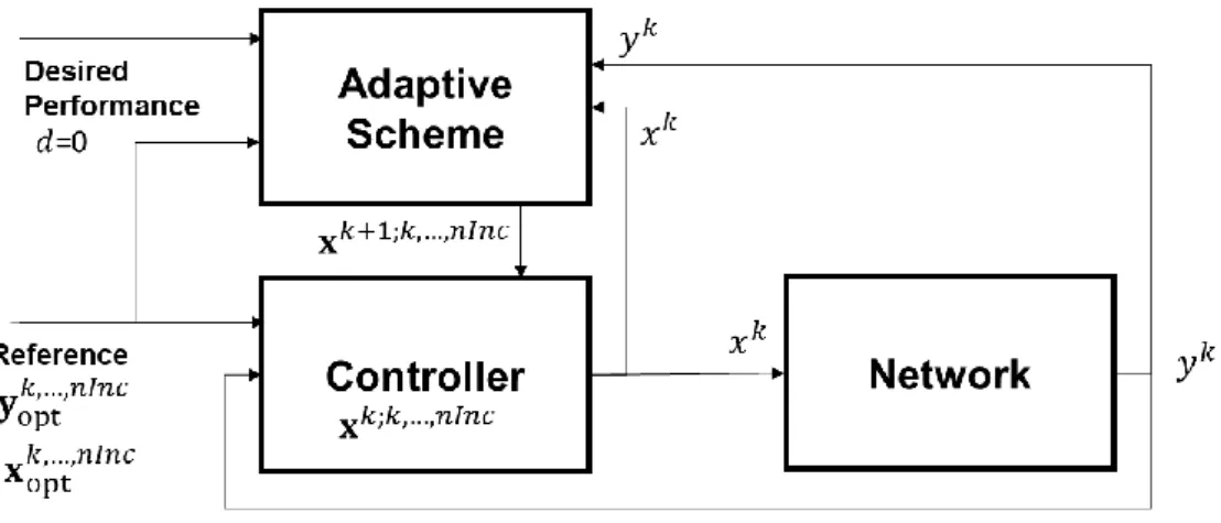
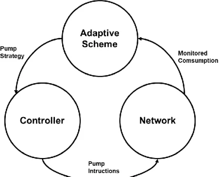
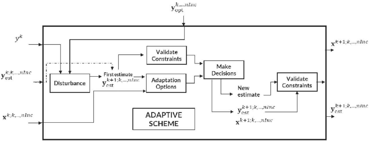
The proposed control model follows a standard adaptive controller architecture, such as the one represented in figure 7. The controller is the combination of 3 main modules: (i) the controller module, (ii) the network module, and (iii) the adaptive scheme module. These modules are in constant interaction with each other. This interaction is sequential, as it is represented in figure 8. The cycle is repeated at every control increment 𝑘, this is the chosen amount of time at which the adaptive controller monitors de network and performs adaptations.

Typically, the amount of time used for the control increment 𝑘 ranges from 15 minutes to 1 hour, corresponding to 𝑛𝐼𝑛𝑐 = 96 𝑜𝑟 24 control increments 𝑘, in a 24-hour day, respectively.

Fig. 7 – Adaptive control architecture.

At every control increment 𝑘, the controller module executes the pumping instructions x𝑘;𝑘,…,𝑛𝐼𝑛𝑐_{by sending information about the amount of time the pumps}

are switched on 𝑥𝑘_{to the network module. The network module receives and}

executes the instructions and sends the monitored water level of the tank 𝑦𝑘 to the adaptive scheme module. The adaptive scheme uses this information to produce a new pumping strategyx𝑘+1;𝑘,…,𝑛𝐼𝑛𝑐 that better adjusts to the demands. This new strategy is then sent to the controller module to execute in the next control increment 𝑘 + 1.

The network module is the water distribution network itself, which can be seen as a plant with unknown parameters inside. The plant responds to a specific input, the amount of pumping 𝑥𝑘, by delivering a measured output, the amount of water consumed by the network or the water level in the tanks 𝑦𝑘.

(39)

15

Fig. 8 – Flow sequence of the adaptive controller.

The controller module receives the updates, and operates by executing one of the following four decisions:

1- No adaptation – The controller doesn’t receive a new pumping strategy

x𝑘+1;𝑘,…,𝑛𝐼𝑛𝑐_{, therefore executes the instructions} _𝑥𝑘_{of its current strategy}

x𝑘;𝑘,…,𝑛𝐼𝑛𝑐_{. This might happen in the case where there is missing information,}

and the adaptive scheme fails at creating a new pumping strategy to feed the controller;

2- Adaptation – The controller receives a new pumping strategy x𝑘+1;𝑘,…,𝑛𝐼𝑛𝑐and follows the instructions 𝑥𝑘 for that control increment 𝑘;

3- Non-routine operation – the disturbance is substantially higher than expected and might signal future problems. The controller starts operating with a different strategy to assure reliability;

4- Send alarm – The monitored water consumption is significantly higher than expected, send an alert for help.

The adaptive controller continuously executes this set of actions in order to reliably and efficiently control the network by facing the changes in consumption when compared with the forecast.

(40)

16

2.2 Adaptive Scheme

Given the nature of the problem, the methodology focusses on meta-heuristics that follow the principles of adaptive algorithms to achieve the desired result. The following sub-sections explain each of the ideas used to develop the algorithm in the adaptive scheme.

2.2.1 Hierarchy Control Update

To produce the most cost-efficient results in energy consuming processes, it’s necessary to take into consideration the tariffs of electricity over the day. Standard tariffs have periods of time where the price of electricity is highest and periods where the price is lowest. Table 1 suggests an example of a possible tariff. As it can be observed in table 1, for the same energy consumed, the cost can be up to 3 times higher. This observation can be extracted by comparing the cost of electricity between a very empty period and peak hours. Therefore, for the same process, the electricity bill differs depending on its timing.

Table 1 – Price tariff over the day.

This is the central concept used to calculate an optimized pumping strategy x_opt𝑘,…,𝑛𝐼𝑛𝑐. The adaptive scheme should update the pumping strategy x𝑘;𝑘,…,𝑛𝐼𝑛𝑐 by seeking the most cost-efficient options, this way assuring that the new pumping strategy x𝑘+1;𝑘,…,𝑛𝐼𝑛𝑐 aims at being cost-efficient. Practically, this means that the pumping strategy x𝑘;𝑘,…,𝑛𝐼𝑛𝑐 is updated according to the measured disturbance 𝑑 by adding or taking pumping time in the control increment 𝑘 where it is obtained the highest benefit.

For example, if it is measured an excess in water consumption, the algorithm searches firstly for the possibility to increase the pumping time 𝑥 in control increments where electricity price is lowest and then to highest accordingly. Conversely, if it is measured a reduction of water consumption compared with the prediction, it takes firstly pumping time 𝑥 from control increments where electricity price is highest, followed by the lowest.

Interval [h] Period Cost [$/kWh]

[0 , 2 [ Empty 0.0737 [2 , 6 [ Very Empty 0.06618 [6 , 7 [ Empty 0.0737 [7 , 9 [ Full 0.10094 [9 , 12 [ Peak 0.18581 [12 , 24 ] Full 0.10095

(41)

17 The purpose of this idea is to search through the remaining control period of 24 hours the most cost-efficient way to update the pumping strategy x𝑘;𝑘,…,𝑛𝐼𝑛𝑐 based on the measured disturbance 𝑑 while assuring that the water level of the tank stays within the established safe limits. The adaptive scheme is proactively finding the best adaptation solution over the 24-hour control period (or any other considered control period), instead of reacting to the measured disturbance 𝑑 by adapting the strategy in the same control increment 𝑘.

In the end, this means that the adaptation follows an hierarchy-based methodology that prioritizes the system reliability while optimizing for a cost efficient operation. This hierarchy control update p_h𝑘;𝑖,…,𝑙, is created at every control increment 𝑘, in order to continuously make the most optimal decisions based on the forward increments 𝑘, … , 𝑛𝐼𝑛𝑐. Mathematically, this process is described in the following equations.

The first part is to establish the price hierarchy. To achieve this, a hierarchy function that attributes a level to the price of electricity for a given control increment 𝑘 is used . This level is an integer that ranges from 1, … , 𝑛 where 𝑛 is the number of different prices of a specific tariff. The scalar 1 indicates the lowest price level and 𝑛 the highest. Mathematically this is described by the following equation,

𝐭_p = hierarchy(𝑘, … , 𝑛𝐼𝑛𝑐), (2)

where 𝐭p is the vector that holds the levels for all control increments 𝑘, … , 𝑛𝐼𝑛𝑐.

Similarly, y_est𝑘;𝑘,…,𝑛𝐼𝑛𝑐 is the vector that contains the estimated water level of the tank for all control increments 𝑘, … , 𝑛𝐼𝑛𝑐 . With this information, it’s possible to compile the hierarchy control update p_h𝑘;𝑖,…,𝑙 using the rankmax and

rank_min functions. The rank_max function sorts the input vector from the highest to the lowest value, and it’s used when the measured disturbance 𝑑 is negative. Conversely the rank_min function sorts the input vector from the lowest to the highest value, and it’s used when the measured disturbance 𝑑 is positive. Mathematically this is described by the following equation;

p_h𝑘;𝑖,…,𝑙= {𝑟𝑎𝑛𝑘max ( 𝐭p × 𝑛𝐼𝑛𝑐 +yest

𝑘;𝑘,…,𝑛𝐼𝑛𝑐_{) for 𝑑 < 0}

𝑟𝑎𝑛𝑘_min ( 𝐭_p× 𝑛𝐼𝑛𝑐 +y_est𝑘;𝑘,…,𝑛𝐼𝑛𝑐 ) for 𝑑 > 0}, (3)

where p_h𝑘;𝑖,…,𝑙 is the vector with that holds the adaptation options ranked from best to worst, 𝑖 is the adaptation option, and 𝑙 = 𝑛𝐼𝑛𝑐 − 𝑘 is the number of adaptation options.

(42)

18

The vector 𝐭_p is multiplied by 𝑛𝐼𝑛𝑐 in order to give it priority over y_est𝑘;𝑘,…,𝑛𝐼𝑛𝑐. This means that the cost of electricity has higher weight in creating the hierarchy control update vector. It is defined the best adaptation the control increment 𝑘

that has the lowest price and the lowest water level of the tank, in case of the 𝑑 > 0, and the control increment 𝑘 that has the highest price and the highest water level of the tank, in case of the 𝑑 < 0.

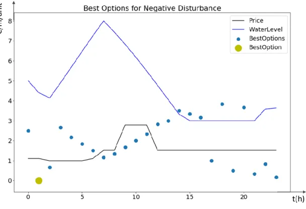
Figures 9 and 10 illustrate the methodology of the hierarchy control updatep_h𝑘;𝑖,…,𝑙. Figure 9 shows the best pumping options found by measuring a negative disturbance 𝑑 in control increment 𝑘 = 0. Figure 10 shows the best pumping options found at measuring a positive disturbance 𝑑 control increment

𝑘 = 0. This example uses 𝑛𝐼𝑛𝑐 = 24 in a 24-hour period.

Fig. 9 – Best pumping options at the control increment 𝑘 = 0 for negative disturbance.

Through analyzing figure 9, it’s clear that the first best pumping options found by the algorithm, when the measured disturbance is negative, are both the ones that have the lowest price and lowest water tank level. Take for example the best adaptation option highlighted by the big yellow circle; a careful analysis shows that it corresponds to the control increment 𝑘 = 2, such that the cost of electricity corresponds to the level 1, and has the lowest water level of the tank among the other control increments belonging to that price level.

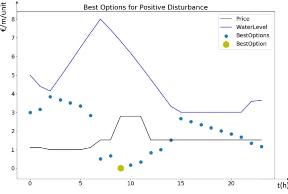
In case that the measured disturbance is positive, then the best adaptation options take a different solution. From figure 10, it can be seen that the hierarchy

(43)

19 methodology finds the opposite answer since it’s more beneficial for the system to decrease pumping time when the electricity price and the water level are highest. Take for an example the best adaptation option highlighted by the big yellow circle; a careful analysis shows that it corresponds to the control increment

𝑘 = 10, such that the cost of electricity corresponds to the level 4, and has the highest water level of the tank among the other control increments belonging to that price level.

In conclusion, the hierarchy pumping idea aims at continuously creating a sorted vector of the best adaptation options that the controller can make to correct the disturbance. This vector can then be used to nullify the disturbance 𝑑, by adding or taking pumping time, starting from the best adaptation option until the worst. This obviously must take into consideration the previous pumping strategy x𝑘;𝑘,…,𝑛𝐼𝑛𝑐_{, in order to make valid adjustments to create the new pumping strategy}

x𝑘+1;𝑘,…,𝑛𝐼𝑛𝑐_.

Fig. 10 – Best pumping options at control increment 𝑘 = 0 for positive disturbance

2.2.2 Sensitivity Analysis

In every control algorithm, it’s necessary to derive a relationship between the control variable (or independent variable) and the observed variable (or dependent variable). In this specific control problem, the control variable is the

(44)

20

amount of time the pumps are switched on, and the observed variable is the water level of the tanks.

Considering now the network as the system to be controlled, that receives the pumping time instructions and outputs the water level of the tank, it’s possible to extract a relation between these variables by testing the sensitivity of the system to the control variable. Mathematically, this is the same to determine the slope of the curve that relates both variables, such as,

∆𝑦= 𝑚 ×∆𝑥, (4)

where 𝑚 defines the pumping time ∆𝑥 for a certain amount of water in the tank ∆𝑦. The most effective strategy to determine the constant 𝑚 is to simulate different pumping strategies in the network with increasing periods of time the pumps are switched on, and then observed the different responses of the system by measuring the water level of the tank. This data set can then be used to calculate a linear regression that describes the system. The following equation defines the process mathematically to determine the relation,

𝑚 =𝑁 × ∑(𝑥 × 𝑦) − (∑ 𝑥) × (∑ 𝑦)

𝑁 × ∑(𝑥2_{) − (∑ 𝑥)}2 , (5)

where 𝑁 is the number of observations used.

For complex systems composed of more than one pumping and tank, this relationship becomes harder to deduct due to the dependencies between all the links and nodes composing the network. In this case the extraction of the tank and pumping relationship becomes more complicated, and it is necessary to recur to a simplification. The strategy focusses on simulating different cases for the states of the pumping in order to derive various points used to determine the constant by the same regression technique mentioned above. The result won’t be as exact; however, it provides a close enough relationship to implement the algorithm. This relation can then be used to transform the measured disturbance

𝑑 in the additional quantity of pumping time ∆𝑥correct to correct it. The amount of

pumping time that is necessary to add or take in order to nullify the observed disturbance is given by,

∆𝑥_correct= 𝑑 × 𝑚. (6)

A seemingly more straightforward approach is to use the pumping equations to determine this relationship. However, this approach is bounded to fail in most cases since it doesn’t take into consideration all the variables of the network that affect the amount of water that is observed in the tank. A straightforward example is the existence of consuming points between the pumps and the tanks that evidently affects how much water is found in the tank. Besides

(45)

21 that, the intrinsic characteristics of the network might also affect the amount of water that reaches the tank. For these reasons, an experimental approach is a better way to study this relationship.

2.2.3 Constraint Validations

The reliability of the operation is more critical than operating a water distribution system in the most cost-efficient way. The water demand of the costumers must always be met. Therefore, the adaptive controller proposed in this work must respect this condition, such that in any adaptation suggested by the adaptation scheme, the water level constraints must be satisfied. The water level safe limits are set accordingly to each specific tank. The limits bound the water level by a minimum and a maximum value, and the control strategy must always take into account these boundaries. This is described mathematically by the following equation,

ℎ_min ≤y_est𝑘+1;𝑘,…,𝑛𝐼𝑛𝑐 ≤ ℎ_max , (7)

where ℎmin is the established lower bound of the water level, ℎmax is the

established upper bound of the water level, and y_est𝑘;𝑘,…,𝑛𝐼𝑛𝑐 is the expected water level for the whole control period of the tank calculated at the control increment

𝑘, which is calculated through,

y_est𝑘+1;𝑘,…,𝑛𝐼𝑛𝑐 = y_est𝑘;𝑘,…,𝑛𝐼𝑛𝑐+ 𝑑. (8)

This objective is partly accomplished with the hierarchy pumping idea since the adaptation in control increments where the water level of the tank is lower is prioritized. However, the cumulative effect of the applied or observed changes are reflected throughout the whole control period and the constraints can’t be validated only considering that idea. Increasing the pumping time 𝑥𝑘_in

the control increment 𝑘 increases the estimated water level of the tank y_est𝑘;𝑘,…,𝑛𝐼𝑛𝑐 for the following increment 𝑘 + 1, … , 𝑛𝐼𝑛𝑐. The cumulative effect of this operation must be addressed by taking into consideration the whole strategy when validating the constraints, such as highlighted in the previous equation. To accomplished this, the following rules are introduced:

1. Adapt before violating

After calculating the expected water level of the tank knowing the impacted of the disturbance 𝑑 by calculating the expected water level of the tank y_est𝑘;𝑘,…,𝑛𝐼𝑛𝑐, it’s possible to determine if any constraint is violated and at which control increment

(46)

22

𝐤_𝑣𝑘,…,𝑛𝐼𝑛𝑐 = {0 for ℎmin ≤ yest

𝑘+1;𝑘,…,𝑛𝐼𝑛𝑐 _{≤ ℎ} max

𝑖 for ℎ_min ≥ y_est𝑘+1;𝑘,…,𝑛𝐼𝑛𝑐 ≥ ℎ_max } , (9)

where 𝐤_𝑣𝑘,…,𝑛𝐼𝑛𝑐 holds the control increments that record the violated constraints. Knowing the point at the which the limits are overpassed, it’s possible to prevent by forcing the adaptation to be done before that control increment 𝑘. Therefore, the valid calculated adaptations by the hierarchy control updatep_h𝑘;𝑖,…,𝑙 are the ones such the respective control increment is smaller than 𝑘 such that 𝑘𝑣𝑘 ≠ 0,

mathematically,

p_hv𝑘;𝑖,…,𝑣 = { p_h𝑘;𝑖,…,𝑙 for p_h𝑘;𝑖,…,𝑙< 𝑘𝑣𝑘} , (10)

where p_hv𝑘;𝑖,…,𝑣 is the valid hierarchy control update vector and holds the sorted control increments 𝑘, from best to worst adaptation, that validates the imposed constraints and 𝑣 is the number of valid adaptation options.

2. React to prevent

The water demand can fluctuate unexpectedly due to random events, such as a fire situation. In this case, the consumption of water might increase radically and, therefore, largely deviate from the forecast. To cope with that situation, the adaptive scheme has a mechanism to prevent the water demand is compromised. Basically, if the measured water consumption is consistently higher (or lower) than the calculated forecast, the adaptive scheme activates a reactive mechanism instead of the established proactive approach to deal with these occasions.

Using this mechanism, the adaptive controller can firmly guarantee the reliability of the operation preventing possible violations of the constraints and reacting to unusual situations.

This mechanism ignores the adaptive scheme actions and reacts by changing the pumping time in the current control increment. This is done using a buffer value that indicates the proximity of the water level to the established limits. This value, which is slightly lower (or higher) than the maximum (or minimum) level of the tank triggers this reactive mechanism. Therefore, the reactive mechanism is triggered if the condition described in the following equation is true;

ℎ_max− 𝑏𝑘 _≤_y

(47)

23 where 𝑏_k is the buffer value at control increment 𝑘.The magnitude of the buffer 𝑏_k

changes over time, and it’s directly proportional to the consistency of the anomaly, such as described in the following equations;

𝑏𝑘 = 𝑗𝑘× 𝑏0, (12)

𝑗𝑘 = {|𝑗

𝑘−1_{+ 1| 𝑓𝑜𝑟 𝑑 > 0}

|𝑗𝑘−1− 1| 𝑓𝑜𝑟 𝑑 < 0}, (13)

where 𝑗𝑘_{is the constant that multiplies by the initially established buffer value}_𝑏 0

at control increment 𝑘 and 𝑗𝑘−1 is the constant that multiplies by the initially established buffer 𝑏₀ of the previous control increment 𝑘 − 1. This mechanism assures the algorithm holds memory of rapid changes in the magnitude of deviations.

2.2.4 Decision-Making Algorithm

The adaptive scheme must be incorporated with a mechanism that determines the best decisions to adapt to the measured disturbance. As highlighted by the previous sections, the decision-making process is bounded to a set of assumptions. To optimally perform this task, the decisions must be made sequentially and properly incorporate every stated principle. figure 11 presents a scheme of the methodology developed. The squared boxes in figure 11 hold the actions performed by the algorithm.

The algorithm starts by calculating the disturbance 𝑑 using the real measure of the water level 𝑦𝑘 and the optimal water level for that control increment 𝑦_opt𝑘 . With that information, an initial estimation of the water level y_est𝑘;𝑘,…,𝑛𝐼𝑛𝑐 for the whole control period is calculated. This information in combination with the previous pumping strategy x𝑘;𝑘,…,𝑛𝐼𝑛𝑐 is used to create the framework of valid pumping update control p_hv𝑘;𝑖,…,𝑣 that is used to make the decisions.

After determining the adaptations that nullify the disturbance, while respecting all the stated assumptions, it’s produced a new pumping strategy x𝑘+1;𝑘,…,𝑛𝐼𝑛𝑐_{and a new estimation of the water level y}

est𝑘+1;𝑘,…,𝑛𝐼𝑛𝑐 for the following

control increment 𝑘. This is again used to validate the constraints in order to predict any future failure of the system as highlighted in the section 2.2.3. At the end of this process, a new pumping strategy for the controller is outputted. The latest estimation of the water level for the whole control period is used to keep track of the influences that the adaptations and disturbance have on the operational strategy.

(48)

24

Fig. 11 – Flow diagram of the decision-making algorithm.

An important note relative to the adaptations in the decision-making process is that the disturbance can be nullified through a set of increments. To accommodate cases where the current strategy doesn’t permit the change, such as in situations that 𝑥𝑘_{+ ∆𝑥}

correct> 1 ∪ 𝑥𝑘− ∆𝑥correct < 0, which is impossible

since the input-variable 𝑥𝑘_{is in fact a fraction of time the pumps are on for each}

control increment and thus 𝑥𝑘 _{∈ [0,1]}_{. Also}_y

est𝑘+1;𝑘,…,𝑛𝐼𝑛𝑐+

∆𝑥correct

𝑚 > ℎmax ∪

y_est𝑘+1;𝑘,…,𝑛𝐼𝑛𝑐 −∆𝑥correct

𝑚 < ℎmin would violate the imposed constraints of the

system, and therefore are not valid. For such cases, the adaptations can be distributed by various control increments such that validates the constraints of the system. In this case, it is necessary to calculate an additional variable that indicates the maximum possible change for a particular control increment 𝑘, as described by; 𝐱adp= { (1 −x𝑘;𝑖,…,𝑙) for 𝑑 > 0 ∩ (y_est𝑘;𝑖,…,𝑙+(1 −x 𝑘;𝑖,…,𝑙₎ 𝑚 ) ≤ ℎmax (x𝑘;𝑖,…,𝑙) for 𝑑 < 0 ∩ (y_est𝑘;𝑖,…,𝑙−(x 𝑘;𝑖,…,𝑙₎ 𝑚 ) ≥ ℎmin 0 else } , (14)

where 𝑥_adp𝑖 is the amount of pumping time that can be taken or added for that control increment, according to the measured disturbance 𝑑. This value is used to perform the adaptation for that control increment 𝑘 and update the ∆𝑥correct in

the following way;

∆𝑥_correct = ∆𝑥_correct− 𝑥_adp,𝑖 (15)

where 𝑖 is the current iteration of the decision-making process and 𝑙 is the iteration number such that ∆𝑥_correct= 0.

(49)

25 This is translated into a sequence of adaptations starting by adapting as much as possible in the first adaptation option of the valid hierarchy update control vector p_hv𝑘;𝑖,…,𝑣 until finally, the disturbance is fully nullified.

(50)

(51)

27

3 Validation, Results, and Discussion

The methodology designed in this work can assure a reliable and cost-efficient control of the operation. The tests are performed by simulating an environment that mimics the behavior of a real water distribution network through software modeling techniques. This enables the extraction of results that can be extrapolated to real WDN. The results are compared with other controllers to provide information about the performance of the adaptive controller across a set of relevant criteria.

3.1 Implementation

Two example networks are used to implement the controller and analyses its performance. The first case study applies the adaptive controller in an elementary network composed of a tank and pump. The second case study uses a simplified version of the benchmark Richmond network, which is composed of 7 pumps and 6 tanks.

3.1.1 Simulation Framework

As explained in the methodology, the adaptive controller is composed of three modules. For simulation purposes, each module has to be modeled through software. The adaptive scheme module and the controller module are the algorithms developed in the methodology. The network module must be represented virtually by shaping the environment of a real network.

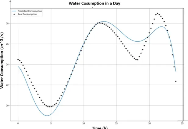
The subsystem F is an excellent framework to test new ideas given its simplicity. The results for this case-study mainly help understand and validate the methodology, not necessary to extrapolate the methodology to real-world scenarios. The scheme of the first network is represented in figure 12 [26]. Since the system is relatively simple, the hydraulic model was implemented using Python. For simulation purposes, and since the adaptive scheme uses a prediction of the water consumption of the system, the modeling framework uses two hydraulic models, one to give the “real” readings at every control increment and another to extract a 24-hour prediction and optimal pumping schedule.

The difference between these hydraulic models lies in the parameters of the consumption functions. The “real consumptions” of water have slight deviations according to the type of test performed. The prediction is always extracted from the same consumption curve.

(52)

28

For the second case study, the hydraulic model of the Richmond network was used with the Epanet simulator. The scheme of the system is represented in figure 13. The Richmond network is a very well-studied network in the academic arena, and a valuable benchmark to test new methodologies and ideas. Besides that, given its complexity and approximation to the real-world scenarios, the results are helpful to validate a new dimension of the adaptive controller developed for this work, scalability. In a single pump-tank simulation, the relation is very straightforward and easy to explore. In a complex network, the interdependence between the several nodes and links might become the bottlenecks of the operation and the reason for failure. Therefore, this case-study provides better conditions to validate the new methodology.

Fig. 12 – Subsystem F network scheme [26].

The case study 2 uses the capabilities of the Epanet 2.0 software to simulate the environment of this network as virtual real network. The network module interacts with the adaptive controller designed in python through a specific API. Similarly, to the previous case study, the simulation uses the same hydraulic model to extract the forecasted consumption for the 24-hours, and the “real consumption” at every control increment. The water consumption forecast is always the same, and for this case study a fully optimized pumping schedule is not used, but rather a typical pumping strategy. The measured water consumption depends on the test performed.