Denis Altieri de Oliveira Moraes
Gráficos de Controle para o
Monitoramento do Vetor de Médias em
Processos Gaussianos Espaço-temporais
Denis Altieri de Oliveira Moraes
Gráficos de Controle para o
Monitoramento do Vetor de Médias em
Processos Gaussianos Espaço-temporais
Tese apresentada ao Departamento de Esta-tística do Instituto de Ciências Exatas da Uni-versidade Federal de Minas Gerais, como re-quisito parcial para a obtenção de Título de Doutor em Estatística.
Área de concentração: Estatística e Probabi-lidade
Orientador: Prof. Dr. Luiz Henrique Duczmal
Co-orientador: Prof. Dr. Fernando Luiz Pe-reira de Oliveira
Moraes, Denis A. O.
Gráficos de Controle para o Monitoramento do Vetor de Médias em Processos Gaussianos Espaço-temporais
112páginas
Tese (Doutorado) - Instituto de Ciências Exatas da Uni-versidade Federal de Minas Gerais. Departamento de Esta-tística.
1. Controle de qualidade
2. Gráfico de controle
3. Vetores de médias
4. Observações individuais
v
Agradecimentos
Agradeço aos meu orientadores, Prof. Luiz Duczmal e Prof. Fernando de Oliveira,
bem como aos demais valiosos colaboradores, pelo incentivo, sugestões e críticas positivas
que culminaram na presente tese. Aos muitos colegas de estudos, os quais demonstraram
grande generosidade durante o andamento das disciplinas mais difíceis, particularmente
a Rodrigo Reis e Reinaldo Marques. Aos meus pais, Delci e Eneli (in memorium),
por proverem amorosamente desde meu nascimento todas as condições para que esse
trabalho se realizasse. Especialmente agradeço a Cláudia Cavalcante, por compartilhar
meus dias e noites, ouvindo pacientemente todos os detalhes de minhas tempestades
racionais. Finalmente, à Universidade Federal de Santa Maria e ao Programa de
Resumo
Nessa tese são apresentadas análises comparativas de cartas de controle tradicionais
e também novos métodos para o monitoramento dos vetores de médias em processos
multivariados. O trabalho aborda os gráficos de controle multivariados para o
monito-ramento do vetor de médias de processos gaussianos com observações individuais. O
controle estatístico do processo em que apenas uma observação está disponível a cada
instante do tempo é um problema de difícil abordagem, já que não é possível detectar
precisamente o deslocamento do vetor de médias por cartas do tipo Shewhart. Nesse
caso é imprescindível o uso de cartas do tipo não-Shewhart, ou seja, considerar no
ins-tante atual a informação proveniente de observações passadas. Nesse sentido, diversos
experimentos foram inicialmente realizados com o propósito de verificar a robustez dos
métodos tradicionais baseados no parâmetro de não-centralidade. Foram investigadas
alternativas ao método mais utilizado em aplicações práticas, o método MEWMA,
com o uso de janelas deslizantes para a detecção de mudanças no vetor de médias do
processo. Finalmente, foram propostos nesta tese novos gráficos de controle, também
baseados no parâmetro de não-centralidade, contudo utilizando uma transformação
linear mais eficiente que o método Análise de Componentes Principais. Verificou-se
através de simulações de Monte Carlo que a estatística de controle proposta preenche
uma lacuna existente quanto à aplicação dos métodos automáticos para o controle do
vetor de médias de processos multivariados, sendo mais eficiente em termos de rapidez
de detecção das mudanças do que os gráficos tradicionais em diversas situações.
Palavras-chave: Controle de qualidade, gráficos de controle, vetores de médias,
vii
Abstract
In this work we present comparative studies as well as new proposals on methods for
statistical process control. Specifically, multivariate control charts with emphasis on
monitoring the mean vector of Gaussian processes with individual observations. The
statistical process control where only one observation is available at each instant of
time is a difficult problem to approach, since it is not possible to accurately estimate
the current process centre by means of Shewhart-type control charts, in which case
it is essential to utilise non-Shewhart control charts, i.e., to consider at the current
instant also information from past observations. Regard to this, several experiments
were initially carried out in order to verify the robustness of the traditional methods
based on the non-centrality parameter. Next, we investigated alternatives to the most
common method used in practical applications, the MEWMA scheme, such as sliding
window schemes for estimation of the current mean vector of the process. Finally, new
control charts have been proposed, also based on the non-centrality parameter, but
utilising a different criterion to obtain a linear transformation, more efficient than the
known method Principal Component Analysis. It was found through experiments that
the proposed statistics fills a gap regarding to the application of automata schemes
for monitoring the centre of multivariate processes, being more efficient in terms of
speed detection of shifts than the traditional quadratic approaches for a wide range of
distances.
Keywords:Quality control, control charts, mean vectors, gaussian processes,
2.1 Fitted linear regressions for control chartŠs calibration utilising known parameters . . . 18
2.2 Empirical in- and out-of-control run length distributions . . . 21
2.3 Empirical in- and out-of-control run length distributions . . . 22
2.4 Diagram of the proposed mean vector shifts for non-correlated and cor-related processes . . . 23
2.5 Shift size with respect to the noncentrality parameter in the correlated and non-correlated processes . . . 25
2.6 The control chartsŠ performance for the three simulated processes and mean vector shifts as noncentrality values . . . 26
2.7 Control chart patterns for moderate and large mean vector shifts . . . . 27
2.8 Control chart patterns for mean vector shifts and increased variances . . 28
2.9 Three-dimensional scatter plots and control charts with confidence el-lipses for a purely autocorrelated out-of-control process Φ = (0.8,0.8) . . 31
2.10 Three-dimensional scatter plots and control charts with confidence el-lipses for the negative autocorrelated process Φ = (⊗0.8,⊗0.8) . . . 32
3.1 Confidence control chart for individual vectors (SW1) with scatter plots 52
ix List of Figures
3.3 Confidence control charts withÚ= 0.7, SW2,𝜙= 0.7 and the respective scatter plots (M1= (3,0)) . . . 55
3.4 Confidence control charts withÚ= 0.4, SW4,𝜙= 0.7 and the respective scatter plots (M1= (3,0)) . . . 57
3.5 ARL and ln(ARL) comparison for all control charts . . . 58
3.6 Comparison for SW1, MEWMA.7, SW2, MEWMA.4 and SW4 schemes 59
3.7 Comparison of mean values of the MEWMA and SW control charts . . 59
3.8 Mean value and standard deviation of the Confidence MEWMA control chart for the in-control process with various ÚŠs . . . 60
3.9 Mean value and standard deviation of the Confidence MEWMA control chart for the out-of-control process with various ÚŠs. . . 61
3.10 Transitional phase comparison for 𝑑 = 0 with MEWMA.1 and SW20 schemes . . . 62
3.11 Transitional phase comparison for 𝑑 = 1 with MEWMA.1 and SW20 schemes . . . 62
3.12 Transitional phase comparison for 𝑑 = 3 with MEWMA.1 and SW20 schemes . . . 63
4.1 Emptiness property of the centre of multivariate spaces . . . 69
4.2 HotellingŠs 𝑇2, MEWMA and Lin-MEWMA control chart patterns with scatter plots (𝑝= 2, Ú= 0.1, 𝑑= 0) . . . 86
4.3 MCUSUM and CUSUM-Lin control chart patterns (𝑝= 2, Ú= 0.1, 𝑘=
0.5, 𝑑= 0) . . . 88
4.4 HotellingŠs 𝑇2, MEWMA and Lin-MEWMA control chart patterns with scatter plots (𝑝= 2, Ú= 0.1, 𝑑= 1) . . . 89
0.5, 𝑑= 1) . . . 91
4.7 MCUSUM and CUSUM-Lin control chart patterns (𝑝= 2, Ú= 0.1, 𝑘=
0.5, 𝑑= 2) . . . 92
4.8 Control chart ARL comparison on the logarithmic scale . . . 97
List of Tables
2.1 Confidence level, estimated thresholds, ARL0 and standard errors for a
Phase II 𝑇2-control chart . . . 19
2.2 Asymptotic thresholds of HotellingŠs 𝑇2 Phases I and II . . . 19
2.3 Adjusted linear regression models with sample estimates and known parameters . . . 20
2.4 Average run length for mean vector shifts with sample estimates and known parameters . . . 24
2.5 Average run length for mean vector shifts with known parameters and correlated processes . . . 26
2.6 The influence of increasing the process variances on the average run length 28
2.7 The ARL influence of simultaneously increasing the variances and shifting the mean vector . . . 29
2.8 The ARL influence of purely increasing autocorrelation levels . . . 30
2.9 The ARL influence of simultaneously increasing variances and shifting the mean vector . . . 30
3.1 Weights computation for sliding window schemes with size 4 (SW4) . . 51
3.2 Weights for sliding window schemes with size 2 (SW2) . . . 51
3.3 Summary of HotellingŠs 𝑇2 and SW1 statistics with ARL comparison. . 53
3.6 ARL comparison between MEWMA and SW control charts . . . 56
4.1 A numerical example of bivariate quality-control schemes (Ú= 0.1) . . . 85
4.2 Control chart performance comparison (𝑝= 2, Ú= 0.1) . . . 93
4.3 Control chart performance comparison (𝑝= 2, Ú= 0.4) . . . 94
4.4 Control chart performance comparison (𝑝= 4, Ú= 0.1) . . . 95
4.5 Control chart performance comparison (𝑝= 4, Ú= 0.4) . . . 96
4.6 Comparison of the performance of the CUSUM-Lin and Lin-MEWMA control charts (𝑝= 2) . . . 100
Nomenclature
Ð The confidence level.
¯
x0 The Phase I in-control estimated mean vector.
Σ The covariance matrix.
Σ0 The in-control variance-covariance matrix.
ä2 The Chi-squared probability distribution.
Δ The difference for the variance of the process 𝑖.
Ó The autocorrelation difference.
𝜖 The Bayes error.
Ò𝑖2 The noncentrality parameter in the MCUSUM control chart.
Ú The smoothing parameter in the MEWMA control chart.
M The mean vector difference from the in-control process.
ARL0 The in-control average run length.
ARL1 The out-of-control average run length.
æ The statistical class or process.
Φ The autocorrelation level.
Ψ The mean vector difference in the MCUSUM control chart.
𝜌 The correlation coeficient.
à𝑖 The variance of the process𝑖.
A The generic scatter matrix.
e The eigenvector of a scatter matrix.
M0 The in-control mean vector.
M𝑡 The current mean vector at the instant𝑡.
S0 The Phase I in-control variance-covariance matrix.
X The generic observed vector.
x𝑖 The individual observation vector.
𝜙 The smoothing constant in the exponential sliding window scheme.
Õ The noncentrality distance when the parameters are estimated.
𝑎 The linear coeficient of regression.
𝐵 The number of Monte Carlo simulations.
𝑏 The angular coeficient of regression.
𝐶𝑡+ The positive CUSUM-Lin statistic.
xv List of Tables
𝑑2 The noncentrality parameter.
𝑓𝑖 The density distribution of the𝑖process.
ℎ The in-control limit.
𝑘 The minimum difference in the MCUSUM control chart.
𝐿𝑖 The 𝑖-th. class.
𝑚 The number of sample vectors.
𝑁 The first occurrence of the alarm.
𝑝 The data dimensionality.
𝑃𝑖 The a priori probability of the class 𝑖
𝑝𝑡 The confidence control chart statistic at the instant 𝑡.
𝑞𝑖 The a posteriori probability of the class 𝑖.
𝑟(X) The conditional error.
𝑟2 The coefficient of determination in the regression model.
𝑠 The weight of the class 𝑖in the Chernoff distance.
𝑤 The weight of the observed vector in the sliding window scheme.
𝑋𝑡 The Lin-MEWMA statistic at the instant 𝑡.
𝑧2
1 Introdução 1
1.1 Apresentação . . . 1
1.2 Principais contribuições . . . 2
1.3 Organização da Tese . . . 4
2 On the Hotelling’s𝑇2, MCUSUM and MEWMA Control Charts’ Per-formance with Different Variability Sources: A Simulation Study 7 2.1 Introduction. . . 8
2.2 Control Charts Methodology . . . 11
2.2.1 HotellingŠs𝑇2 Control Chart . . . . 12
2.2.2 Multivariate Cumulative Sum Chart . . . 13
2.2.3 Multivariate Exponentially Weighted Moving Average Chart. . . 14
2.2.4 Confidence Ellipse Estimation by Principal Component Analysis 15 2.3 Experiments and results . . . 16
2.3.1 Control chart calibration . . . 17
2.3.2 In-control and out-of-control run length distributions. . . 20
2.3.3 Performance comparison for mean vector shifts . . . 23
2.3.4 The influence of increasing variances . . . 27
2.3.5 The influence of autocorrelation . . . 29
xvii Contents
3 Confidence Control Charts with MEWMA and Sliding Window Schemes 37
3.1 Introduction. . . 38
3.2 Methodology . . . 41
3.2.1 A review on the HotellingŠs𝑇2 and MEWMA control charts. . . 41
3.2.2 Upper bounds on the error probability . . . 44
3.2.3 The confidence control charts . . . 48
3.2.4 Confidence control chart with MEWMA scheme . . . 49
3.2.5 Confidence control chart with sliding window schemes . . . 49
3.3 Experiments and results . . . 51
3.4 Discussion . . . 64
4 Self-oriented Control Charts for Efficient Monitoring of Mean Vec-tors 67 4.1 Introduction. . . 68
4.1.1 Control charts for Gaussian processes . . . 70
4.1.2 The noncentrality parameter . . . 72
4.2 Methodology . . . 73
4.2.1 Maximisation criteria . . . 75
4.2.2 The Lin-MEWMA control chart . . . 79
4.2.3 The CUSUM-Lin control chart . . . 81
4.3 Experiments and results . . . 82
4.3.1 Control chart calibration procedure. . . 83
4.3.2 A numerical example . . . 84
4.3.3 Control chart pattern analysis. . . 85
4.3.4 Performance comparison . . . 93
5.1 Considerações finais . . . 105
5.2 Trabalhos futuros . . . 107
Capítulo 1
Introdução
1.1
Apresentação
O início da revolução industrial, em torno dos anos 1800, foi marcado principalmente
pela transição entre os lentos processos de produção artesanais para a produção em
série com o uso de máquinas. Sendo um divisor de águas, a manufatura de itens de
consumo em larga escala mudou de forma sem precedentes na história o panorama social
e econômico da humanidade. Com o desenvolvimento tecnológico, surgiram próximo
dos anos 1900 as rápidas máquinas a vapor, e com elas também a necessidade de evitar
desperdícios controlando os processos automatizados de produção.
Sendo o principal nome associado aos estudos da área hoje denominada Controle
Estatístico de Qualidade, Walter A. Shewhart, enquanto trabalhava na empresa Bell
Telephones em 1925, foi pioneiro no uso de métodos estatísticos para decidir quando
uma ação corretiva deveria ser aplicada a um processo. Seu principal trabalho nesse
sentido foi publicado em 1931 no livroEconomic Control of Quality of Manufactured
Product (Shewhart,1931).
Apoiado no alto poder computacional disponível atualmente para o rápido
forma, a presente tese tem como objetivo contribuir com para a melhoria dos métodos
para o controle estatístico de qualidade, enriquecendo de forma global o grande universo
do qual fazemos parte.
1.2
Principais contribuições
A abordagem das contribuições apresentadas nessa tese desenvolveu-se gradual e
cres-centemente. Inicialmente foi investigado os padrões de comportamento dos métodos
tradicionalmente aplicados na indústria para o monitoramento do vetor de médias de
um processo gaussiano. Nesse estudo introdutório foi analisado o comportamento dos
limites de controle dos gráficosmultivariate cumulative sum (MCUSUM),multivariate
exponentially weighted moving average (MEWMA) e 𝑇2 de Hotelling quando são
uti-lizadas amostras de tamanho limitado proveniente da Fase I, e também considerando
parâmetros conhecidos. Nesse sentido, foi observado que para lidar com a maior variação
dos dados, os limites de controle tendem a aumentar à medida que períodos menores
da Fase I são utilizados. A seguir, foi verificado que os gráficos de controle estudados
são afetados de forma diferenciada quando diferentes fontes de variação ocorrem nos
processos. Particularmente, o gráfico de controle de Hotelling apresenta maior
sensibili-dade para a detecção do aumento de variâncias no processo que os demais, enquanto
os gráficos MCUSUM e MEWMA são mais sensíveis ao aumento de autocorrelação
positiva nos processos. Apesar disso, os gráficos MCUSUM e MEWMA não apresentam
nenhuma sensibilidade quanto a detecção da ocorrência de autocorrelação negativa em
qualquer nível, efeito somente detectado pelo gráfico de Hotelling.
Em uma segunda etapa, foram propostos gráficos de controle de confiança, os
quais derivam de uma relação probabilística das distâncias tradicionais, não limitadas
3 1.2. Principais contribuições
propor uma nova interpretação para as distâncias dos gráficos tradicionais, foi também
útil para a análise e criação de uma correspondência o parâmetro de suavização Ú,
utilizado no gráfico MEWMA, e o tamanho de janelas deslizantes na estimação do vetor
de médias. Embora útil, o tamanho da janela deslizante é um importante parâmetro até
então de difícil escolha por parte do analista, que influencia diretamente a magnitude
da mudança a ser detectada.
Também com a utilização dos gráficos de confiança, foi analisado o problema do
efeito inercial que ocorre nos gráficos do tipo não-Shewhart. Tal efeito inercial pode ser
compreendido como um retardamento na detecção de mudanças de grande magnitude,
quando comparados à velocidade de detecção do método Shewhart. Nesse sentido, foi
identificado que diferentemente do que podem suspeitar alguns pesquisadores, o uso
de janelas deslizantes não reduz o efeito inercial em métodos não-Shewhart. Embora
as janelas deslizantes sejam amplamente aplicadas em identificação de padrões comuns
em certos processos, como sazonalidade e alternação de sinais, foi averiguado que seu
uso amplifica o efeito inercial, retardando assim a detecção de grandes mudanças nos
processos.
A principal contribuição desta tese recai sobre o problema da redução e seleção de
variáveis do processo através de transformações lineares, geralmente realizado através
da técnica conhecida como Análise de Componentes Principais (ACP). Destaca-se que
com a aplicação da metodologia proposta no final desta tese para os gráficos de controle,
foi possível obter uma redução significativa no efeito inercial. Nesse contexto, sabe-se
que a ACP não fornece uma regra definitiva para o problema sobre quais componentes
principais devem ser selecionadas, geralmente acarretando em perda de desempenho
em termos de velocidade de detecção das mudanças. De acordo com a literatura em
reconhecimento de padrões e processamento de sinais, a transformação linear realizada
pelo método ACP é indicada para a representação de sinais, não sendo eficiente quando
classi-uma redução de dimensionalidade mais efetiva. Como a implementação de tal critério
na área de controle de processos era até o momento desconhecida, os experimentos com
os novos gráficos de controle propostos evidenciaram que há de fato uma seleção ótima
da direção a ser monitorada, tornando a redução da dimensão dos processos ótima no
sentido de minimizar o tempo de detecção de mudanças no vetor de médias.
1.3
Organização da Tese
Como destacado anteriormente, o desenvolvimento desta tese deu-se de forma gradual.
A partir do estudo e reconhecimento dos padrões de atuação dos métodos clássicos
no monitoramento da média de processos multivariados, foram sendo estudadas as
possibilidades de modificação desses métodos até o desenvolvimento bem sucedido de
um novo método de controle.
Assim, o trabalho foi elaborado em três etapas, sendo que cada uma delas resultou em
um artigo autônomo, aqui organizado sequencialmente como um único volume. Como
os trabalhos foram elaborados independentemente, alguns conteúdos introdutórios aos
métodos estão apresentados novamente nas três partes principais da tese.
No Capítulo 2 são apresentados os três métodos clássicos no monitoramento do
vetor de médias de processos multivariados. Nesse capítulo é proposto um método de
calibração comum, o estudo dos limites de controle e os padrões de desempenho dos
gráficos de controle tradicionais frente a diferentes fontes de variabilidade.
O Capítulo 3 apresenta os gráficos de controle de confiança e também investiga a
utilização das janelas deslizantes como abordagem alternativa para minimizar o efeito
inercial dos gráficos de controle. Nesse contexto é apresentado de forma clara uma
relação entre o parâmetro de suavização do método MEWMA e o tamanho das janelas
5 1.3. Organização da Tese
de médias de processos multivariados, denominadas de Lin-MEWMA e CUSUM-Lin,
são apresentadas no Capítulo 4. Finalmente, o Capítulo5 faz um resumo do trabalho
realizado e expõe novos objetivos e planejamentos a ser implementados em futuros
Chapter 2
On the Hotelling’s
T
2
, MCUSUM
and MEWMA Control Charts’
Performance with Different
Variability Sources: A Simulation
Study
Abstract
This work is a simulation study to investigate the sensitivity of multivariate control
charts for monitoring mean vectors in a bivariate Gaussian process with individual
observations. The multivariate cumulative sum (MCUSUM), the multivariate
expo-nentially weighted moving average (MEWMA) and HotellingŠs 𝑇2 charts are selected
for analysis due to their common dependency on the noncentrality parameter. The
or Phase I sample estimates is considered for mean vector shifts. Although designed
to monitor mean vectors, the sensibility of the control charts is additionally analysed
through different variability sources, including the mixing effect of mean vector shifts
with increasing variances or positive autocorrelation in the out-of-control process.
2.1
Introduction
Developed to study the influence of social castes in India in the early 20th century,
the Mahalanobis (1936) distance is an important example of a dissimilar metric in various disciplines. Among many existing applications of this distance, in the statistical
process control (SPC) it is known as the noncentrality parameter. With the increase in
computational power over the last century and the growing number of applications, the
Monte Carlo method can help to understand its behaviour under different simulated
scenarios.
In SPC, the noncentrality parameter is frequently used in control charts to detect
process changes, triggering a signal as soon as the underlying process shifts from the
in-control state to the out-of-control state. To evaluate the control chart performance,
the metric typically adopted is the average run length (ARL) or average time to signal
(ATS). The ATS is the process ARL when the time interval between samples is fixed
at one time unit, as during this simulation study.
An important factor for rapid change detection is selecting the correct method, which
depends on the available data and the change to be monitored. Montgomery (2001)
elaboration of the decision schemes is a main reference to correctly choose a control
chart method. Lowry and Montgomery(1995) present an additional review. Although
the multivariate exponentially weighted moving average (MEWMA) of Lowry et al.
9 2.1. Introduction
popular and more suitable to detect small changes, the𝑇2 chart is suggested to monitor
the mean vector for large-scale shifts. Mahmoud and Maravelakis (2010; 2011) use
estimates of the parameters for evaluating the performance of two types of MCUSUM
and MEWMA control charts. These charts are based on the noncentrality parameter
and can be applied to a number𝑝 of variables, where𝑝⊙1. When 𝑝= 1, all methods
are reduced to their respective univariate schemes, which are CUSUM, EWMA and X
control charts. Recent work proposes several chart modifications, such as the double
exponentially weighted moving average (dEWMA) method proposed by Alkahtani and
Schaffer (2012).
To monitor the covariance matrix, Montgomery (2001) recommends the moving
range and generalised variance tests,Riaz and Does(2008) suggest utilising supporting
information andCosta and Machado (2008) postulate the VMAX procedure. Quinino
et al.(2012) also propose a single statistic based on the mixture of variances (VMIX)
to monitor the covariance matrix of bivariate processes. Yeh et al. (2006) proposed
modifications of the EWMA method based on the generalised variance.
The approaches for simultaneously monitoring changes in the mean vector and the
covariance matrix are numerous, and we highlight the integration of the exponentially
weighted moving average procedure with the generalised likelihood ratio test ofZhang
et al.(2010) andKhoo et al.(2010), whose statistics are based on the maximum of the absolute values of the two dEWMA statistics, one of which controls the mean vector
and the other the covariance matrix. The numerous proposals to monitor changes in the
mean vector of autocorrelated data (Montgomery,2001) include traditional methods
that fit the time series and subsequently implement control techniques on the model
residuals produced by the fit.
Although designed to monitor mean vector shifts, the present study analyses the
sensibility of the MCUSUM, MEWMA and HotellingŠs𝑇2 statistics for process changes
for mean vector shifts is compared considering known parameters or training on small
samples sizes. The simulated mean vector shifts includes comparisons about the shiftŠs
direction in correlated and non-correlated processes with known parameters. Increasing
variances and the influence of a vector autoregressive model are additionally measured
and analysed using the ARL value, keeping the mean vector fixed.
The bivariate case is chosen to analyse the multivariate point process for their broad
application in space-time problems and to provide a general example of multivariate data.
Another positive aspect of studying only two variables is the visual potential to identify
the in- and out-of-control observations in their original spaces in three-dimensional
observations to make more direct conclusions and facilitate the understanding of what
occurs in the higher-dimensional spaces. To emphasise this objective, Lowry and
Montgomery(1995) recommends extending additional graphical approaches, including
the Polyplot method (Blazek et al., 1987), beyond the HotellingŠs 𝑇2 statistic and
including techniques, as the MEMWA chart, that effectively detect small changes.
Although different methodologies for data visualization are employed together with the
control charts, this work presents a tool for continuous data view in the scatter-plots,
estimating confidence ellipses for the current process based on principal component
analysis (PCA).
In Section 2, we present a review of the noncentrality parameter, which is the
common distance used in the HotellingŠs𝑇2, MCUSUM and MEWMA control charts
is presented. Additionally we provide a brief explanation of PCA as a tool for data
visualisation in the scatter-plots. Section 3 analyses results of experiments for different
shifts in the mean vector with known parameters or sample estimates. As inertia
problems may occur in non-Shewhart control charts, our recommendation is the use
of simultaneous non-Shewhart and Shewhart-type control charts to avoid detection
delay. Further, the ARLs measure the chart sensibility due to increasing variances,
11 2.2. Control Charts Methodology
shifts. The final section discusses the control charts performance and sensibility in the
proposed scenarios and prospects for future work.
2.2
Control Charts Methodology
In the general case, suppose that vectors x1,x2,x3, . . . of dimension 𝑝×1 represent
sequential observations of𝑝characteristics over time. The observationsx𝑖,𝑖= 1, 2, . . . ,
are assumed to be independent random vectors of a multivariate normal distribution
with a mean vectorM0 and covariance matrixΣ0. Without loss of generality, consider
that M0= (0,0,. . . ,0) =0 and Σ0 =I.
The HotellingŠs 𝑇2, MCUSUM and MEWMA control charts analysed share the
property that their performances, as measured by ARL, depend on MandΣexpressed
as the noncentrality parameter𝑑(Lowry et al.,1992), which is given by
𝑑2 =M′Σ⊗1M (2.1)
WhenΣ0is the identity matrix,𝑑is reduced to a Euclidean distance. In his original
formulation, Hotelling suggests the utilisation of𝑑2 to avoid the labor of extracting the
square root. If the in-control process is not symmetrical around its centre of mass, as
occurs for correlated variables, the Euclidean distance does not consider the process
covariance, thus making it directionally dependent. To quantify the magnitude of
shifts without directional dependence, the shifts should be correctly weighted by the
covariance matrix. The statistical pattern recognition literature (Therrien,1989) shows
that the noncentrality parameter, also known as the Mahalanobis distance, is related
to other statistical measures as the Divergence (D) and Bhattacharyya (B) distances.
When the covariance matrices of two processes are equal, then 𝑑2 =𝐷= 8𝐵.
For the composite problem, each observation is compared within two or more classes
and attributed to the one with the shortest distance. The noncentrality parameter in
a control chart evaluates the relative vector distance to the in-control process mean.
Thus, problems related to the control charts often arise as single hypothesis tests, i.e.,
when the unique known class is the in-control state. The analysis of signals from radar
devices is an example of single hypothesis tests applied in the pattern recognition field,
when the aim is the simple recognition of potential targets.
Note the existence of two implicit assumptions in the performance comparisons
based on the noncentrality parameter. First, any shift, regardless of size, must be
detected as early as possible. Second, a shift from M0 to M1 is detected as quickly as
a shift from M0 to M2 ifM′1Σ0⊗1M1 =M′2Σ⊗01M2. As the ARL value is a function
of the noncentrality parameter 𝑑, the comparisons between the methods are simplified
with analysis of the curve ARL vs. 𝑑. Alternatively, if the charts do not share this
property, their relative performance may vary depending on Σ, i.e., even for a given
matrix Σ, a chart may more effectively detect changes in some directions and less
effectively in other directions.
2.2.1 Hotelling’s T2 Control Chart
The statistic proposed by Hotelling (1947) triggers a signal when there is a significant
shift in the mean vector, such that
𝑑𝑖2 = (x𝑖⊗M0)′Σ0⊗1(x𝑖⊗M0)> ℎ1 (2.2)
where ℎ1 >0 is the threshold specified to maintain a desired in-control average run
length (ARL0).
13 2.2. Control Charts Methodology
for the HotellingŠs 𝑇2 statistics. When we assume that the observations x𝑖 are not
time-dependent and that the process parameters are known, 𝑑2𝑖 follows a Chi-squared
distribution with 𝑝 degrees of freedom and then ℎ1 = ä2(𝑝,1⊗Ð) (Seber, 1984). This
is a a Phase II control chart called 𝑇2-chart for individual observations with known
parameters.
If𝑚 samples are used to compute (¯x0,S0), the estimates of (M0,Σ0) andx𝑖 is an
individual observation that is not independent of the estimators, then the 𝑑2𝑖/𝑑0(𝑚)
statistic follows a Beta distribution with 𝑝/2 and (𝑚⊗𝑝⊗1/2) degrees of freedom,
where 𝑑0(𝑚) = (𝑚⊗1)2𝑚(⊗1) and𝑝 is the data dimension. Thus, the upper control
limit is given by ℎ1=𝑑0(𝑚)Ñ(1⊗Ð,𝑝/2,(𝑚⊗𝑝⊗1)/2). This control chart is called a Phase I
𝑇2-chart (Tracy et al.,1992).
If the estimators are utilised instead of the parameters and ifx𝑓 is a future individual
observation that is independent of (¯x0,S0), then𝑑2𝑓/𝑑1(𝑚,𝑝) follows an F-distribution
with𝑝and (𝑚⊗𝑝) degrees of freedom, where𝑑1(𝑚,𝑝) =𝑝(𝑚+ 1) (𝑚⊗1) [𝑚(𝑚⊗𝑝)]⊗1.
Thus, the upper control limit of this multivariate Shewhart control chart is𝑑1(𝑚,𝑝)F(1⊗Ð,𝑝,𝑚⊗𝑝).
This control chart is called a Phase II𝑇2-chart with unknown parameters.
Because the multivariate Shewhart control charts only consider the information
given by the current observation, they are insensitive to small and moderate shifts in
the mean vector. To overcome this problem, we concisely describe the multivariate
CUSUM and EWMA schemes proposed in the literature.
2.2.2 Multivariate Cumulative Sum Chart
Among the multivariate CUSUM methods proposed by Crosier (1988), the method
with the best properties in terms of performance triggers an alarm when the statistic
Ò𝑖2=⎞Ψ′𝑖Σ⊗01Ψ𝑖
⎡
where Ψ𝑖 = 0, if 𝐶𝑖 ⊘ 𝑘, Ψ𝑖 = (Ψ𝑖⊗1+x𝑖⊗M0) (1⊗𝑘/𝐶𝑖) if 𝐶𝑖 > 𝑘, Ψ0 = 0,
𝑘 >0 and𝐶𝑖 =
[︁
(Ψ𝑖⊗1+x𝑖⊗M0)′Σ0⊗1(Ψ𝑖⊗1+x𝑖⊗M0)
]︁1/2
,𝑖= 1,2,. . .. The upper
control limit ℎ2 is determined to provide a predefined in-control ARL by simulation.
Because the ARL performance of this chart depends on the noncentrality parameter,
Crosier recommends𝑘=𝑑/2 for a shift detection of 𝑑units.
2.2.3 Multivariate Exponentially Weighted Moving Average Chart
The MEWMA method proposed by Lowry et al.(1992) is a natural extension of the
EWMA chart. Its multivariate formulation defines the EWMA vector as z𝑖 =λx𝑖+
(I⊗λ)z𝑖⊗1 = ∑︀𝑖𝑗=1λ(I⊗λ)𝑖⊗𝑗x𝑗, 𝑖 = 1,2,. . ., where z0 = 0, the initial in-control
mean vector of the process, and λ = 𝑑𝑖𝑎𝑔(Ú1,Ú2,. . . ,Ú𝑝), 0 ⊘ Ú𝑗 ⊘ 1, 𝑗 = 1,2,. . . ,𝑝.
Whenλ=I, the MEWMA control chart is equivalent to the𝑇2-chart. Similar to other
methods, this procedure triggers an out-of-control signal when
𝑧𝑖2 =⎞z′𝑖Σ⊗01z𝑖 ⎡
> ℎ3 (2.4)
where ℎ3 > 0 is chosen by simulation to obtain a predefined value of ARL0 and
Σ(zi) is the covariance matrix ofz𝑖. If there is no reason to differentially weight the
his-torical observations in the𝑝characteristics, thenÚ1,Ú2,. . . ,Ú𝑝=Úis utilised, but when
unequal weighting constants are considered, the ARL depends on the direction of the
shift. The covariance matrix ofz𝑖 is calculated asΣ(zi)=
∑︀𝑖
𝑗=1Var
[︁
λ(I⊗λ)𝑖⊗𝑗x𝑗 ]︁
=
∑︀𝑖
𝑗=1λ(I⊗λ)𝑖⊗𝑗
′
Σ(I⊗λ)𝑖⊗𝑗λ; when Ú1 = Ú2 = ... = Ú, Σ(zi) =
⎞
1⊗(1⊗Ú)2𝑖⎡
(Ú/(2⊗Ú))Σ. An approximation of the variance-covariance matrix Σ(zi) as 𝑖
ap-proaches +∞ is given as Σ(zi) = Ú/((2⊗Ú)Σ0); however, the appliance of exact
15 2.2. Control Charts Methodology
chart.
2.2.4 Confidence Ellipse Estimation by Principal Component
Analy-sis
The principal components method is a common multivariate procedure for projecting
the original variable space into an orthogonal space, so less transformed variables that
represent different sources of variation can be monitored together with multivariate
control charts or individually with univariate control charts (Bersemis et al., 2007).
Among the applications of this very useful method in multivariate quality control,
Jack-son (1991) studied three types of control charts based on PCA. The first type is a
𝑇2-control chart obtained from principal scores components, the second is a control
chart for principal component residuals and the third is a control chart for each
inde-pendent principal componentŠs scores. Thus, further analysis could be made to monitor
individual observations using their projections into the principal components. Bersemis
et al. (2007) offer a detailed description of multivariate process control via PCA and other projection techniques. Making a distinction between signal classification and
signal representation as exposed by Fukunaga (1990), the authors applies PCA as a
descriptive tool, establishing in- and out-of-control regions for the current process and
then visualization helps to an understand the process in conjunction with the control
charts.
PCA aims to find a matrixΣ* with a linear transformation ofΣ, which rotates the
original axes in the directions of decreasing (or increasing) variability. In the bivariate
case, the eigenvectore1 = (e11,e12) associated with the first principal component (𝑃 𝐶1)
in the rotation matrixΣ*indicates the direction of maximum process variability, and the
first eigenvaluev1 indicates the normalised size of variation in that direction. Similarly,
the second principal component (𝑃 𝐶2) indicates the direction and magnitude of the
To plot the in- and out-of-control ellipses in the scatter-plots showed in the present
work, take the rotation angle of the estimated ellipse (in radians) with respect to the
original coordinate system from the trigonometric rules, such as the arctangent of the
first eigenvector, which points in the direction of greatest variability. Similarly, the
second eigenvector provides the direction of the second most significant variation. The
estimated axis sizes in the directions of the major and minor variability are normalised,
and the eigenvalues are multiplied by the quantile of a multivariate normal distribution
to establish the confidence region of (1⊗Ð) 100%, where Ð is the error probability.
Assuming that the subjacent process is Gaussian, we adopt 𝑧(1⊗Ð) = 3.023, which
corresponds to an errorÐ = 0.005 for the estimated axis size. The in-control ellipses
are drawn in blue and the out-of-control ellipse in red.
2.3
Experiments and results
As described above, the calibration of the MCUSUM and MEWMA charts to obtain
a predefined value for ARL0 involves defining the 𝑘-factor in the MCUSUM and Ú
in the MEWMA. For the MCUSUM chart, Crosier (1988) notes that one should
choose𝑘=𝑑/2 to detect a shift with a magnitude 𝑑corresponding to the noncentrality
parameter. For the MEWMA method, Lowry et al.(1992) illustrate optimal schemes
to choose the weighting factor Ú, which generally must be in the [0.05; 0.25] range.
According to the authors, the optimum suggested value ofÚto detect a unitary change
in the noncentrality parameter is 0.16. In the present work,Ú= 0.1 is selected for the
MEWMA chart as this value is a common choice in several papers to compare with
the MCUSUM chart utilising𝑘= 0.5 (which corresponds to a target shift detection of
noncentrality value 𝑑= 1).
Set the𝑘 and Úvalues, the control limitsℎ𝑖 are estimated for the control charts to
17 2.3. Experiments and results
calibrated to an ARL0 of 200, which is an intermediate value for the mean time, after
which a false alarm may be triggered. Defining in-control thresholds for each chart
using the same ARL0 ensures an equivalent type I error for the tests under the null
hypothesis of no change in the process.
As the calibration procedure is complete, we compare the chart ARL1 values, i.e.,
the chart performance with a shift in the process. When the underlying process is
actually out-of-control with a mean vector shift, a smaller ARL1 value corresponds to
better chart performance. Conversely, the chart may trigger a signal for a different
variation source, indicating that the chart is not robust for different causes of variation.
Thus, the ARL1 computed for other sources of variation and different mean vector
shifts can be viewed as a disadvantage or lack of robustness of the chart and treated as
a scale of sensibility. The ARL empirical computation is described in the next section.
All routines for the experiments are elaborated using the R language (Development
Core Team,2008).
As previously stated, the HotellingŠs 𝑇2-control chart calibration is achieved using
the process sample estimates or the known parameters to compute the thresholds by
means of asymptotic distributions. An additional HotellingŠs 𝑇2-control chart
calibra-tion observes the false alarm rate and computes the probability of a signal, but we
do not apply this procedure because the non-Shewhart control charts do not share
this signal independence property. To compare the performance of non-Shewhart and
Shewhart-type control chart, we choose the method described below in lieu of the
tra-ditional Markov Chain or integral equations approach for the MCUSUM and MEWMA
threshold estimation.
2.3.1 Control chart calibration
In this work, the control chart calibration is computed by specifying a sequence of
average run length (ARL0). Then, a linear regression model in the form ln (𝐴𝑅𝐿) =
𝑎+𝑏×ℎ𝑖 is fitted to estimate the target threshold for a predefined ARL0 = 200.
(a) (b) (c)
Figure 2.1: Fitted linear regressions for control chartŠs calibration utilising known parameters
To access the ARL0 estimation for each threshold value, the number of samples𝑚
is set equals 2,000. This quantity of observations show high probability (> 99.9% for
ARL0 = 200) of triggering a false alarm when the process is actually in-control. When
observed, the positionN of the first alarm occurrence is recorded as the run length, and
the mean value of N, computed fromB Monte Carlo simulations, is the ARL0 for that
threshold. In the experiments performed with known parameters and 20,000 Monte
Carlo simulations, the maximum observed run length is 1,844. To avoid missing values
when the signal does not occur, 𝑚 is set to a maximum of 2,000. The experiments
are performed with B = 2,000 Monte Carlo simulations to speed up the regression
adjustment step, and B = 20,000 are performed with the estimated in-control limit for
the final ARL0 and ARL1 computation.
To illustrate the threshold sensitivity in the HotellingŠs 𝑇2-control chart, Table2.1
contains the asymptotic values for a Phase II control chart, based on theF distribution,
and respective standard errors obtained in 100,000 Monte Carlo simulations, where
𝑚= 100 observations of the in-control process were simulated each step for parameter
estimation. The highest threshold (ℎ0.999 = 15.13) corresponds to an ARL0 value of
1,000 observations. Similarly, the confidence level of 99.5% (ℎ0.995= 11.42) shows an
19 2.3. Experiments and results
Table 2.1: Confidence level, estimated thresholds, ARL0 and standard errors for a
Phase II 𝑇2-control chart
(1⊗Ð) 100% ℎ1 ARL0 SE
99.9 15.13 1000.1 3.127
99.5 11.42 200.7 0.625
99.0 9.85 99.7 0.316
95.0 6.30 19.9 0.063
With the asymptotic values of Table 2.2for the HotellingŠs𝑇2-chart and the
refer-ence values in the original papers for the MEWMA and MCUSUM charts, the linear
regressions displayed in the Figure 2.1are fitted with known parameters for all chartsŠ
calibrations. The minimum number of threshold values for the regression estimation is
10, and the maximum is 18. The values along the vertical axes are ARL0 values in a
logarithmic scale, and the values along the horizontal axes are the in-control limits. The
parameter estimation is carried out with 𝑚= 25, 50 and 100 for the number of Phase I
samples of individual observations. The thresholds value sequences for estimating the
regression model of each control chart are set to approximate the ARL0 between 100
and 300. All fitted regressions, goodness-of-fit and estimated thresholds for a target
ARL0 = 200 are shown in Table2.3.
Table 2.2: Asymptotic thresholds of HotellingŠs 𝑇2 Phases I and II
Asymptotic distribution
m ä2-distribution Beta-distribution F-distribution
25 - 8.81 14.61
50 - 9.69 12.34
100 - 10.14 11.42
(M0,Σ0) 10.60 -
-We first compare the estimated thresholds with the asymptotic values of HotellingŠs
𝑇2 control charts presented in Table 2.2. In Table 2.3, we notice that the linear
expected, and the estimate for known parameters (10.61) is very close to the asymptotic
value (10.60). Second, for sample estimates, the regression adjusted thresholds are close
to the asymptotic average between the two distributions. For𝑚= 25, the asymptotic
threshold average is 11.71, while the regression estimate is 11.26. For 𝑚= 50 and 100,
the asymptotic threshold averages are 11.02 and 10.78, respectively, while the regression
estimates are 10.93 and 10.60. Thus, the linear regression approach is effective for
calibrating HotellingŠs𝑇2-control chart.
Table 2.3: Adjusted linear regression models with sample estimates and known param-eters
Control Chart m Fitted model 𝑟2 ^ℎ𝑖 = (𝐴𝑅𝐿0)
𝑇2 25 𝑙𝑛(ARL0) = 0.3710*ℎ1+ 1.1206 0.956 11.26
50 𝑙𝑛(ARL0) = 0.4628*ℎ1+ 0.2414 0.971 10.93
100 𝑙𝑛(ARL0) = 0.4954*ℎ1+ 0.0463 0.985 10.60
(M0,Σ0) 𝑙𝑛(ARL0) = 0.4773*ℎ1+ 0.2351 0.992 10.61
MCUSUM 25 𝑙𝑛(ARL0) = 0.5138*ℎ2+ 1.7467 0.974 6.91
50 𝑙𝑛(ARL0) = 0.6589*ℎ2+ 1.1829 0.993 6.25
100 𝑙𝑛(ARL0) = 0.7343*ℎ2+ 0.9318 0.997 5.95
(M0,Σ0) 𝑙𝑛(ARL0) = 0.8611*ℎ2+ 0.5451 0.986 5.52
MEWMA 25 𝑙𝑛(ARL0) = 0.2811*ℎ3+ 2.0399 0.963 11.59
50 𝑙𝑛(ARL0) = 0.3628*ℎ3+ 1.5648 0.974 10.29
100 𝑙𝑛(ARL0) = 0.3892*ℎ3+ 1.5511 0.994 9.63
(M0,Σ0) 𝑙𝑛(ARL0) = 0.4348*ℎ3+ 1.4904 0.993 8.76
2.3.2 In-control and out-of-control run length distributions
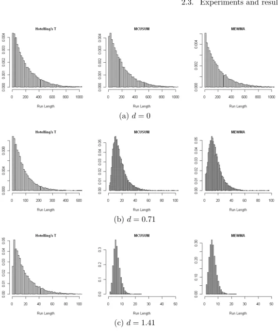
To compare the run length distributions calibrated with known parameters, Figure2.2
presents a sequence of density histograms based on the resulting run length values for
20,000 Monte Carlo simulations. Figure 2.2(a) shows the run length distributions for
the three control charts and the first moment of each distribution are the ARL0 values
of the last group in Table2.4, which is based on the known parameters (M0,Σ0).
Some large observations are not displayed in the histograms because the horizontal
21 2.3. Experiments and results
(a)𝑑= 0
(b)𝑑= 0.71
(c) 𝑑= 1.41
Figure 2.2: Empirical in- and out-of-control run length distributions
the HotellingŠs 𝑇2 is clearly the most favourable to change detection. The run length
distribution of the MEWMA control chart as seen Figure 2.2(b)-(c) confirm that this
control chart with Ú= 0.1 tends to perform better than the MCUSUM with 𝑘= 0.5.
This result is also confirmed by the ARL1 values produced in the experiments with
known parameters of Table2.4.
(a) 𝑑= 2.12
(b)𝑑= 2.82
(c)𝑑= 3.54
Figure 2.3: Empirical in- and out-of-control run length distributions
run length distributions. For the ARL1estimation, the total number of simulated sample
observations (𝑚) utilised for each mean vector shift was 1,500, 1,000, 500, 200 and 100,
23 2.3. Experiments and results
2.3.3 Performance comparison for mean vector shifts
Excluding the specific mean vector shifts to test the MCUSUM method,Crosier(1988)
evaluates𝑑unitary increments in the 0 to 5 range for several dimensions. Lowry and
Montgomery (1995) in the MEWMA method evaluate shifts through𝑑increments in the 0 to 3 range. The present work simulates changes in equal increments for both
dimensions, and the centre of the process is shifted diagonally from (0.0, 0.0) to (2.5,
2.5) by increments of 0.5 in both dimensions, representing𝑑values in the 0 to 3.54 range.
The probability inside the area defined by three standard deviations in a non-correlated
process is 0.995.
Figure2.4illustrates the proposed mean vector shifts for correlated and non-correlated
processes. The non-correlated scheme in Figure 2.4 is calibrated with estimated and
known parameters. The correlated variable schemes of Figure 2.4are compared only
for the case of known parameters. The experienced reader should argue why to do
comparisons with correlated variables since the charts performance does not depends
on the shifts direction. For that reasoning, the authors intend to emphasize that a shift
of magnitude 𝑑is different when it occurs in the process directions of major and minor
variability.
● ●● ●
y1 y2
−4 −2 0 2 4 6
−4
−2
0
2
4
6
● ●
● ●
● ●
● ●
y1 y2
−4 −2 0 2 4 6
−4
−2
0
2
4
6
● ●
● ●
● ●
● ● ● ●
y1 y2
−4 −2 0 2 4 6
−4
−2
0
2
4
6
● ●
● ●
● ●
For non-correlated processes shown in Figure 2.4, the in-control limits are delimited
with known parameters and sample estimates of three different sizes (𝑚= 25; 50; 100)
in Phase I. Table 2.4 presents the resulting in- and out-of-control ARLs. Although
the standard error (SE) of the estimate is relatively large for the ARL0 due to the
regular number of Monte Carlo simulations (𝐵 = 20,000), the ARL1 values show little
variation.
The main observed effect due to the utilisation of small sample sizes to train the
control chart in Table2.4is an increasing delay in the change detection as the sample
size decreases. The MCUSUM and MEWMA charts perform very similarly for all shifts,
with faster performance than the HotellingŠs 𝑇2-chart for the shifts (2.0, 2.0) that are
situated around the target noncentrality value (𝑑= 1). To this point, the inertia effect
begins to delay the change detection for the non-Shewhart charts, and the shift for the
point (2.5, 2.5) is more likely to be detected with the Shewhart-type control chart.
Table 2.4: Average run length for mean vector shifts with sample estimates and known parameters
d 0 0.71 1.41 2.12 2.82 3.54
m Chart ARL0 ARL1 ARL1 ARL1 ARL1 ARL1
MCUSUM 199.4 26.3 7.3 4.5 3.3 2.6
25 MEWMA 201.1 28.1 7.8 4.7 3.4 2.7
𝑇2 199.3 91.7 26.5 7.7 3.1 1.7
MCUSUM 197.3 20.2 6.8 4.2 3.1 2.5
50 MEWMA 199.1 20.9 7.1 4.4 3.3 2.6
𝑇2 199.9 87.3 21.9 6.6 2.8 1.6
MCUSUM 203.1 18.2 6.4 4.0 3.0 2.4
100 MEWMA 200.3 18.4 6.8 4.2 3.1 2.5
𝑇2 200.6 84.2 20.5 6.3 2.7 1.5
MCUSUM 198.6 16.0 6.0 3.7 2.8 2.3
(M0,Σ0) MEWMA 197.2 15.2 5.8 3.6 2.7 2.1
𝑇2 201.0 76.9 18.6 5.7 2.5 1.5
25 2.3. Experiments and results
the changes only in the first quadrant, thus allowing changes to represent both large
and small shifts respective to the noncentrality parameter. Figure2.5demonstrates how
much those different structures allow the same shift in the mean vector to represent
a relatively different shift in the noncentrality parameter. Compared with the
non-correlated process represented by the solid line, the mean vector shifts measured by the
noncentrality parameter are smaller in the positively correlated process (gray line) and
larger in the negatively correlated process (dashed line).
Figure 2.5: Shift size with respect to the noncentrality parameter in the correlated and non-correlated processes
Throughout the rest of the experiments, the in-control limits are obtained by
cal-ibrating the control chart with the process known parameters. The results for ARL
comparison in detecting the process shift schemes of Figure2.4 are shown in Table2.5
and represented in𝑑units in Figure2.6. Although the MCUSUM and MEWMA charts
have equivalent performance in the three situations, the performance of the HotellingŠs
𝑇2-chart exceeds the others after the first shift in Figure2.6(c), when the shift occurs in
the minor axis of the negatively correlated process. This result does not contradict the
finding that the HotellingŠs 𝑇2-chart is a better monitor of large shifts. This situation
MCUSUM and MEWMA methods (Lowry et al., 1992), delay change detection and
make the HotellingŠs𝑇2-chart more efficient in the third shifting scheme. We observe
that larger shifts often occur in the direction of larger variability. A more realistic
suggestion in this case is to observe relatively less movement in the direction of minor
variability. The large values in the direction of lower variability are usually related to
typing errors in the data acquisition procedure (Montgomery,2001). An observation
of the point where the charts intersect indicates that the relative magnitude of the
changes in all three cases is the same when measured using the noncentrality parameter
(𝑑≍= 2.6).
Table 2.5: Average run length for mean vector shifts with known parameters and correlated processes
d 0 0.71 1.41 2.12 2.82 3.54
𝜌 Chart ARL0 ARL1 ARL1 ARL1 ARL1 ARL
MCUSUM 200.8 26.8 9.0 5.3 3.8 3.0
0.85 MEWMA 202.0 25.0 8.7 5.1 3.7 2.9
𝑇2 203.9 112.8 38.9 14.3 6.2 3.2
MCUSUM 199.7 4.4 2.2 1.6 1.2 1.0
-0.85 MEWMA 201.1 4.3 2.1 1.5 1.2 1.0
𝑇2 201.5 9.0 1.4 1.0 1.0 1.0
(a) 𝜌= 0 (b)𝜌= +0.85 (c) 𝜌=⊗0.85
Figure 2.6: The control chartsŠ performance for the three simulated processes and mean vector shifts as noncentrality values
27 2.3. Experiments and results
The changes in the processes are moderate and large shifts. The inertia effect can
be viewed in Figure 2.7(b) with the non-Shewhart control charts. As the HotellingŠs
𝑇2-chart triggers a signal at the very first out-of-control observation, the MCUSUM
and MEWMA charts are affected by a delay in triggering the signal.
● ● ● ● ● ● ● ● ● ● ● ●●●● ● ● ●● ●● ● ● ● ● ● ● ● ●● ● MCUSUM
0 5 10 15 20 25 30 35 40 45 50
0 5 10 15 ● ● ● ● ● ● ● ● ●● ● ● ● ●● ●● ● ●● ● ● ● ● ● ● ● ● ●● ● ● ● ● MEWMA
0 5 10 15 20 25 30 35 40 45 50
0 5 10 15 20 ● ● ● ●● ● ● ● ● ● ● ● ●● ● ● ● ● ●● ● ● ● ● ● ● ● ● ● ● ● ● ● ● ●● ●● ● ● ● ● ● ● ●● ● ● ● T 2
0 5 10 15 20 25 30 35 40 45 50
0 5 10 15 ● ● ● ● ● ● ● ● ● ● ● ● ● ● ● ● ●● ● ● ● ● ●● ● ● ● ● ● ● ● MCUSUM
−4 −2 0 2 4
−4 −2 0 2 4 ● ● ● ● ● ● ● ● ● ● ● ● ● ● ● ● ●● ● ● ● ● ●● ● ● ● ● ● ● ● ● ● ● MEWMA
−4 −2 0 2 4
−4 −2 0 2 4 ● ● ● ● ● ● ● ● ● ● ● ● ● ● ● ● ● ● ● ● ●●●● ● ● ● ● ● ● ● ● ● ● ●● ● ● ● ● ● ● ● ● ● ● ● ● ● T2
−4 −2 0 2 4
−4
−2
0
2
4
(a)𝑑= 1.41,M1 = (1.0,1.0)
● ● ● ● ● ● ● ● ● ● ● ● ● ● ● ● ● ● ● ● ●● ● ● ● ●
●
MCUSUM
0 5 10 15 20 25 30 35 40 45 50
0 10 30 50 70 ● ● ● ● ● ● ● ● ● ● ● ● ● ● ● ● ● ● ● ● ● ● ● ● ● ● ●● MEWMA
0 5 10 15 20 25 30 35 40 45 50
0 50 100 150 ● ● ● ● ● ● ● ●● ● ● ●● ●● ● ●●● ● ● ● ● ● ● ● ● ● ● ● ●● ● ● T 2
0 5 10 15 20 25 30 35 40 45 50
0 5 10 15 20 25 ● ● ● ● ● ● ● ● ● ● ● ●● ● ● ● ● ● ● ● ● ● ● ● ● ● ● MCUSUM
−4 −2 0 2 4
−4 −2 0 2 4 ● ● ● ● ● ● ● ● ● ● ● ●● ● ● ● ● ● ● ● ● ● ● ● ● ● ● ● MEWMA
−4 −2 0 2 4
−4 −2 0 2 4 ● ● ● ● ● ● ● ● ● ● ● ●● ● ● ● ● ● ● ● ● ● ● ● ● ● ● ● ● ● ● ● ● ● T2
−4 −2 0 2 4
−4
−2
0
2
4
(b) 𝑑= 3.54,M1= (2.5,2.5)
Figure 2.7: Control chart patterns for moderate and large mean vector shifts
2.3.4 The influence of increasing variances
If the variances of the underlying process changes from (à2
1,à22) to
)︃
à2
1+ Δ,à22+ Δ
)︀
=
)︃
à2
1,à22
)︀*
, control chart may be affected because this overdispersion increases the
indi-vidual observation distances with respect to the center of the in-control process. The
results in Table 2.6reflect the effect of process variance increases, which demonstrates
a larger influence on the HotellingŠs𝑇2-control chart.
The patterns that result from simultaneously altering the mean vector and
covari-ance matrix generate a greater tendency for signal growth than the pattern shown
in Figure 2.8(a). When the mean vector changes, the subsequent process changes
stemming from the modification of the covariance matrix greatly influence the chartsŠ
pro-Table 2.6: The influence of increasing the process variances on the average run length
)︃
à21,à22)︀*
(1.0, 1.0) (1.5, 1.5) (2.0, 2.0) (2.5, 2.5)
Control chart ARL0 ARL1 ARL1 ARL1
MCUSUM 198.1 52.3 26.8 17.9
MEWMA 202.8 56.3 29.0 18.9
𝑇2 202.3 35.0 14.2 8.4
cess to be out-of-control, beginning with the characterisation of a new centre of gravity,
the HotellingŠs 𝑇2-chart discriminates all of the observations that exceed the coverage
area, as defined by the in-control process.
●●●●● ●● ● ● ● ●● ●●
● ● ●●● ● ●●
●● ●●●●
MCUSUM
0 5 10 15 20 25 30 35 40 45 50
0 5 10 15 20 25 30 ● ● ● ●● ●● ● ● ● ● ● ● ● ● ● ● ● ● ● ● ● ● ● ●●● ● MEWMA
0 5 10 15 20 25 30 35 40 45 50
0 10 20 30 40 50 60 ● ● ●● ● ● ● ● ●● ●● ● ● ● ● ● ● ● ● ● ● ● ● ● ● ● ● ● ● ● ● ● ● ● ● ● ● ● ● ● ● ●● ● ● ● ● T 2
0 5 10 15 20 25 30 35 40 45 50
0 5 10 15 ● ● ● ● ● ● ● ● ● ● ● ● ● ● ● ● ● ● ● ● ● ● ● ●●● ● ● MCUSUM
−4 −2 0 2 4
−4 −2 0 2 4 ● ● ● ● ● ● ● ● ● ● ● ● ● ● ● ● ● ● ● ● ● ● ● ● ● ● ● ● MEWMA
−4 −2 0 2 4
−4 −2 0 2 4 ● ● ● ● ● ● ● ● ● ● ● ● ● ● ● ● ● ● ● ● ● ● ● ● ● ● ● ● ● ● ● ●● ● ●● ● ● ● ● ● ● ●● ● ● ● ● T2
−4 −2 0 2 4
−4 −2 0 2 4 ●●● ● ● ● ● ● ● ● ●●● ● ● ● ● ●●●● ● ● ● ●● ● ● ●● MCUSUM
0 5 10 15 20 25 30 35 40 45 50
0 10 20 30 40 ● ●●● ● ● ● ● ● ● ●● ● ● ● ● ● ●● ● ●●● ● ● ● ● ● ● ● ● MEWMA
0 5 10 15 20 25 30 35 40 45 50
0 20 40 60 80 ●● ●● ● ● ● ● ● ● ●● ●● ● ● ● ●●● ●● ● ● ● ● ● ● ●● ● ●●● ● ● ● ● ● ● T 2
0 5 10 15 20 25 30 35 40 45 50
0 10 30 50 ● ● ● ● ● ●● ● ● ● ● ● ● ● ● ● ● ● ● ● ● ● ● ● ● ● ● ● ●● MCUSUM
−4 −2 0 2 4
−4 −2 0 2 4 ● ● ● ● ● ●● ● ● ● ● ● ● ● ● ● ● ● ● ● ● ● ● ●● ● ● ● ●● ● MEWMA
−4 −2 0 2 4
−4 −2 0 2 4 ● ● ● ● ● ●● ● ● ● ● ● ● ● ● ● ● ● ● ● ● ● ● ● ● ● ●● ● ● ● ● ● ● ● ● ● ● ● ● T2
−4 −2 0 2 4
−4
−2
0
2
4
(a)M1 = (1.0,1.0),Σ1 =
⎟
1 0 0 1
⟨
(b)M1 = (1.0,1.0),Σ1 =
⎟
2 0 0 2
⟨
Figure 2.8: Control chart patterns for mean vector shifts and increased variances
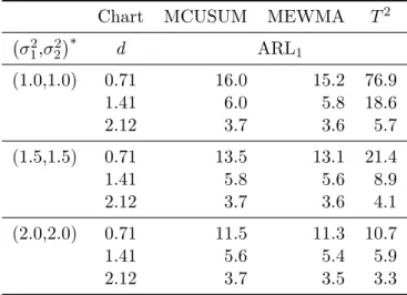
The difference in the chartsŠ performance can be observed by comparing Table 2.6
and 2.7. Table 2.7 shows the influence of variance increasing over the mean vector
shifts. This experiment performs only a slight increase in the variances, which changes
from )︃
à12,à22)︀
= (1.0,1.0) to)︃
à12,à22)︀*
= (1.5,1.5). The combined effect of the increased
variances and mean vector shifts is more evident for the HotellingŠs𝑇2 control chart,
where the reductions in the ARL1 are expressive. The MCUSUM and MEWMA control
29 2.3. Experiments and results
ARL1 reduction for the non-Shewhart charts in the second shift is less significant for
bigger shifts.
Table 2.7: The ARL influence of simultaneously increasing the variances and shifting the mean vector
Chart MCUSUM MEWMA 𝑇2
)︃
à21,à22)︀*
d ARL1
(1.0,1.0) 0.71 16.0 15.2 76.9
1.41 6.0 5.8 18.6
2.12 3.7 3.6 5.7
(1.5,1.5) 0.71 13.5 13.1 21.4
1.41 5.8 5.6 8.9
2.12 3.7 3.6 4.1
(2.0,2.0) 0.71 11.5 11.3 10.7
1.41 5.6 5.4 5.9
2.12 3.7 3.5 3.3
2.3.5 The influence of autocorrelation
To verify the control chartsŠ performance when the process is perturbed with
auto-correlation, the out-of-control processes are simulated based on a first-order
autore-gressive model, VAR(1), on a scale of increasing intensity. The autocorrelations in
both dimensions are Φ = (ã1,ã2) = (0.0,0.0) for the in-control process and Φ =
(ã1+Ó,ã1+Ó) = (Ó,Ó) for the out-of-control process. The autocorrelation levels are
Ó = (0.1,0.2,0.3,0.4,0.5,0.6,0.7,0.8,0.9). The degree of influence on the processes is
indi-rectly evaluated by comparing the ARL1 values produced in the experiments described
in Table 2.8and 2.9to the values presented in Table 2.4, where only the mean vector
was modified.
The experiment in Table2.8demonstrates that pure autocorrelation in the
out-of-control process results in small mean vector shifts, being less noticed by the HotellingŠs