Design and optimization of building integration PV/T systems (BIPV/T)

UNIVERSITY OF ÉVORA

SCHOOL OF SCIENCES AND TECHNOLOGY

DEPARTMENT OF PHYSICS

Design and Optimization of Building Integration

PV/T Systems (BIPV/T)

Ricardo Jorge da Silva Pereira

Supervision: Laura Aelenei, Ph.D.

António Joyce, Ph.D.

Masters in Solar Energy Engineering

Dissertation

Évora, 2015

UNIVERSITY OF ÉVORA

SCHOOL OF SCIENCES AND TECHNOLOGY

DEPARTMENT OF PHYSICS

Design and Optimization of Building Integration

PV/T Systems (BIPV/T)

Ricardo Jorge da Silva Pereira

Supervision: Laura Aelenei, Ph.D.

António Joyce, Ph.D.

Masters in Solar Energy Engineering

Dissertation

Évora, 2015

“The Stone Age came to an end, not because we had a lack of stones”

R

ESUMO

Design e Optimização de um Sistema PV/T Integrado em Edifício (BIPV/T)

Neste trabalho é analisado, por via numérica e experimental, o comportamento térmico e eléctrico de um sistema fotovoltaico/térmico integrado em edifício, recorrendo a material de mudança de fase para regularização da diferença de temperatura entre interior e exterior e para a estabilização da temperatura do módulo fotovoltaico.

Foi realizado uma revisão da literatura sobre o tema. Um modelo de cálculo dos fenómenos de transferência de calor e massa foi desenvolvido, assim como da produção de energia eléctrica, e implementado em software de cálculo Matlab/Simulink®.

Paralelamente foram conduzidos ensaios experimentais a fim de analisar o comportamento térmico do sistema e respectiva validação do modelo numérico. De modo a melhorar a eficiência total do sistema, foi aplicado um processo de optimização com o método dos algoritmos genéticos. Do estudo, conclui-se que o sistema pode alcançar uma eficiência máxima total de 64% na configuração de inverno e de 32% na configuração de verão.

Palavras Chave: Edifício integrado fotovoltaico/térmico; Armazenamento de energia; Material mudança de fase; Modelo térmico; Algoritmo Genético.

A

BSTRACT

This work presents a numerical and experimental analysis of the thermal and electrical performance of a building integrated photovoltaic/thermal system (BIPV/T), with the use of phase change material for stabilize the temperature difference between indoors and outdoors and a rapid stabilization of the PV modules’ temperature.

A literature review was conducted on the topic. A calculation model was developed of the heat and mass transfer phenomena, as well as a model of a photovoltaic module, which were implemented in Matlab/Simulink®.

Experimental tests were performed to analyze the thermal performance of the system and the validation of the numerical model. To improve overall system efficiency, an optimization process with the method of genetic algorithms was applied.

From the study, it is concluded that the system can achieve a maximum total efficiency of 64% with winter configuration and 32% with summer configuration.

Keywords: building integrated photovoltaic/thermal; energy storage; phase-change material; thermal modelling; genetic algorithm.

A

CKNOWLEDGEMENTS

I would like to express my sincere thanks to the various people and entities whose contributions have been of benefit to this work.

I would first like to thank Laura Aelenei, Ph.D., and Professor António Joyce, the scientific mentors of this work, for their permanent monitoring, availability, and critical and constructive spirit.

Thanks, too, to LNEG for giving me the opportunity to take part in this project.

And to my sister Marta Pereira for the scientific support she provided.

Thanks to Luisa for all her support.

Thanks to everyone who contributed in some way to this work. They are: Alvaro Ramalho, Ana Rute, António Rocha e Silva, Bruno Durão, Carlos Rodrigues, and José Ventura. I also would like to thank to Jean Burrows for the English revision of the manuscript.

I am grateful to FogãoSol for constructing the prototype.

I must also thank the Foundation for Science and Technology (FCT) for financial support in the form of research fellowship, under the FRAME project financed by FEDER funds through the Operational Program for Competitiveness Factors - COMPETE and national Funds through FCT - Foundation for Science and Technology under the project FCOMP-01-0124-FEDER-019471 (Ref PTDC/AURAQI-AQI/117782/2010).

T

ABLE OF CONTENTS

RESUMO ... I ABSTRACT ... III ACKNOWLEDGEMENTS ... V TABLE OF CONTENTS ... VII LIST OF FIGURES ... XI LIST OF TABLES ... XV NOMENCLATURE ... XVII INTRODUCTION ...1 CHAPTER 1. 1.1.INTRODUCTION ...1 1.2.OBJECTIVES ...3 1.3.OUTLINE ...3

BUILDING INTEGRATED PV/TSYSTEMS (BIPV/T)REVIEW ...5

CHAPTER 2. 2.1.INTRODUCTION ...5

2.2.INTEGRATION /APPLICATION...6

2.3.APPROACH ... 11

2.4.EFFICIENCY ... 13

BASIC FUNDAMENTALS OF HEAT AND MASS TRANSFER... 15

CHAPTER 3. 3.1.INTRODUCTION ... 15

3.2.HEAT TRANSFER... 15

3.2.1. Conduction Heat Transfer ... 16

3.2.2. Convection Heat Transfer ... 18

3.2.3. Radiation Heat Transfer ... 21

3.3.THERMAL RESISTANCE ... 24

3.4.ENTHALPY TRANSPORT ... 25

3.5.THERMAL MASS ... 25

4.1.INTRODUCTION ... 29

4.1.1. Air velocity within the air cavity... 30

4.1.2. PCM model approach ... 30

4.2.PROBLEM FORMULATION ... 32

4.2.1. Heat Transfer Coefficients ... 32

4.2.2. Thermal Model ... 36

4.2.3. Electrical Model for PV Module ... 38

4.3.SYSTEM PERFORMANCE ... 40

4.4.IMPLEMENTATION OF THE NUMERICAL MODEL IN MATLAB® ... 41

4.4.1. Heat Transfer in Simscape® ... 42

4.4.2. Constructing the Model ... 45

EXPERIMENTAL EVALUATION ... 47

CHAPTER 5. 5.1.INTRODUCTION ... 47

5.2.DESIGN PROJECT ... 48

5.3.SYSTEM DESCRIPTION ... 49

5.4.EXPERIMENTAL SET-UP AND INSTRUMENTATION ... 51

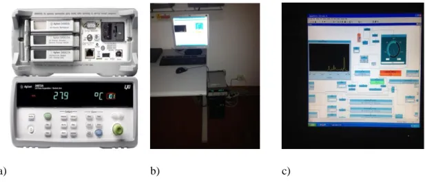
5.4.1. Data Acquisition Logger... 53

5.4.2. Temperature Sensors ... 54

5.4.3. Fluxmeter Sensors ... 56

5.4.4. Hotwire Anemometer ... 58

5.4.5. Thermal Images... 58

5.5.MEASUREMENT CAMPAIGN AND EXPERIMENTAL RESULTS ... 59

5.5.1. Winter Campaign ... 59

5.5.2. Summer Campaign ... 65

5.5.3. Campaigns Comparison ... 70

5.6.VALIDATION OF THE NUMERICAL MODEL... 72

5.6.1. Introduction ... 72

5.6.2. Validation ... 72

5.6.3. Air Velocity Within the Cavity ... 75

5.6.4. System Performance ... 75

SYSTEM OPTIMIZATION ... 79

CHAPTER 6. 6.1.INTRODUCTION ... 79

6.2.OPTIMIZATION METHOD (GA) ... 80

6.3.APPLICATION OF THE METHOD ... 82

6.3.1. Software Application (Matlab) ... 85

6.4.OPTIMIZATION SCENARIOS ... 88 6.5.RESULTS... 90 6.5.1. Winter ... 90 6.5.2. Summer ... 94 6.5.3. Overall ... 98 CONCLUSION... 101 CHAPTER 7. 7.1.DISCUSSION ... 101 7.2.FUTURE WORK ... 103 REFERENCES ... 105 APPENDICES ...A-1 APPENDIX A...A-1 APPENDIX B ...A-1 APPENDIX C ...A-2 APPENDIX D...A-3

L

IST OF FIGURES

Fig. 2.1. Review specific subjects. ...6

Fig. 2.2. Example of a scheme of a water based BIPV/T applied on a facade [17] ...7

Fig. 2.3. Schematic of a BIPV/T applied on a façade – SOLAR XXI Building [30] ...8

Fig. 2.4. Concept schematic for a BIPV/T system with transpired collector [31]. ...9

Fig. 2.5. Example of a scheme of an air-based BIPV/T with PCM, applied on a façade [37] ...9

Fig. 2.6. Schematic of a BIPV/T applied on a roof [6] ... 10

Fig. 2.7. a) Schematic of a water based BIPV/T applied on a roof, b) Schematic of a water based PV/T [49] ... 11

Fig. 2.8. Example of a thermal network of a BIPV/T roof system [6]. ... 12

Fig. 2.9. Example of a CFD simulation flow pattern (left). Example of a CFD simulation PV temperature (right) [28]. ... 13

Fig. 2.10. Graphical summary of the efficiency obtained by the authors. ... 14

Fig. 3.1. Heat transfer through a ventilated air cavity wall system [53] ... 16

Fig. 3.2. One-dimensional heat transfer by conduction [55] ... 17

Fig. 3.3. Boundary layer development in convection heat transfer [55] ... 18

Fig. 3.4. Radiation exchange: a) at a surface and (b) between a surface and large surroundings [55] ... 22

Fig. 3.5. Stages of a phase transition of a PCM ... 27

Fig. 4.1. System configuration... 29

Fig. 4.2. (a) Phase transition curve for a PCM gypsum board from DSC test [63]. (b) Approximation of DSC curve [63] ... 31

Fig. 4.3. Model studied – Thermal network [37] ... 32

Fig. 4.4. PV equivalent circuit [73] ... 39

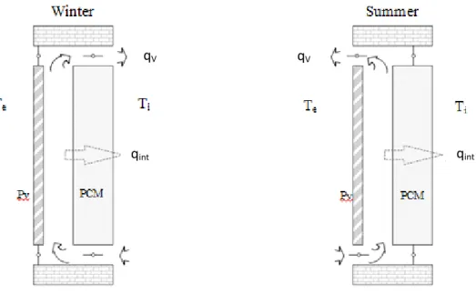
Fig. 4.5. winter (left) and summer (right) configurations... 40

Fig. 4.6. Simscape® Conductive Heat Transfer block ... 43

Fig. 4.7. Simscape® Convective Heat Transfer block ... 43

Fig. 4.8. Simscape® Radiative Heat Transfer block ... 43

Fig. 4.9. Custom Simscape® Convection Heat Transfer block ... 44

Fig. 4.10. Simscape® Thermal Mass block ... 44

Fig. 4.11. Simscape® Solar Cell block ... 45

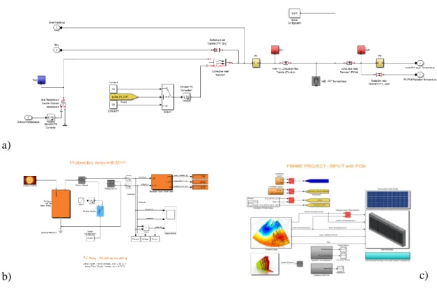
Fig. 4.12. Simscape PV thermal layer block (a), PV electrical model block (b), First window interface (c). ... 45

Fig. 5.1. Solar XXI building (top), Prototype installed on the Solar XXI main facade (bottom)

[37] ... 50

Fig. 5.2. Crosssection of BIPV-PC [35]. ... 50

Fig. 5.3. Cross section set-up and sensor positions [37] ... 52

Fig. 5.4. Sensors installed on inner PV layer (a), Sensors installed on inner PCM layer (b) ... 53

Fig. 5.5. Detail of the support structure for the three air temperature sensors ... 53

Fig. 5.6. Data Logger (a), Data Acquisition apparatus (b), Data logger acquisition software (c) ... 54

Fig. 5.7. PT 100 sensor (a). PT 100 Self-adhesive sensor (b) ... 55

Fig. 5.8. PT 100 sensor (a), PT 100 Self-adhesive sensor (b) ... 55

Fig. 5.9. Hukseflux HFP01 fluxmeter (a). Hukseflux HFP01 fluxmeter installed at PV interior layer (b) ... 56

Fig. 5.10. Hukseflux SR11 pyranometer (a). SR11 pyranometer installed at PV exterior layer (b) ... 57

Fig. 5.11. Hotwire anemometer logger (Testo 425) (a). Taking measurement with the hotwire anemometer (b) ... 58

Fig. 5.12. Testo Fluke Ti25 thermal camera ... 59

Fig. 5.13. Exterior, interior temperature and solar radiation measurements February 2013 [35] ... 60

Fig. 5.14. Temperature and irradiance values, 22 February 2013 [35]. ... 60

Fig. 5.15. Cross section temperatures at different times, 22 February 2013 [35]. ... 61

Fig. 5.16. Heat flux through PCM surfaces 22 February 2013. ... 62

Fig. 5.17. Temperature and irradiation values, 25 February 2013 [35] ... 63

Fig. 5.18. Cross section temperatures at different times, 25 February 2013 [35] ... 64

Fig. 5.19. Heat flux through surfaces, 25 February 2013 ... 64

Fig. 5.20. Exterior, interior temperature and solar radiation measurements, June and July 2013... 65

Fig. 5.21. Temperature and irradiation values, 5 July 2013 ... 66

Fig. 5.22. Cross section temperatures at different times, 5 July 2013 ... 67

Fig. 5.23. Heat flux through surfaces 5 July 2013 ... 67

Fig. 5.24. Temperature and irradiation values, 19 June 2013... 68

Fig. 5.25. Cross section temperatures at different times, 19 June 2013 ... 69

Fig. 5.26. Heat flux through surfaces 19 June 2013 ... 69

Fig. 5.27. Four days’ parameters: Radiation (top left), Exterior temperature (top right); Four days’ data: Heat flux through PCM (bottom left), Air flow system (bottom right) ... 70

Fig. 5.29. 25 February (left); 5 July (right) [37]. ... 72

Fig. 5.30. Simulated versus experimental values of heat flux through layers for 25 February 2013 ... 73

Fig. 5.31. Simulated versus experimental values of heat flux through layers for 5 July 2013 ... 74

Fig. 5.32. Thermal images and photos at 12:00 on 5 July 2013 ... 74

Fig. 5.33. Air velocity within cavity ... 75

Fig. 5.34. Thermal BIPV-PCM system efficiency. 25 February 2013 (left), 5 July 2013 (right) ... 76

Fig. 5.35. Electrical BIPV-PCM system efficiency ... 77

Fig. 6.1. Flowchart of a simple routine optimization through genetic algorithms [79] ... 83

Fig. 6.2. Functional diagram of the optimization toolbox ... 86

Fig. 6.3. Winter configuration for the optimization process... 88

Fig. 6.4. Summer configuration for the optimization process ... 89

Fig. 6.5. Climatic conditions for the optimization process ... 90

Fig. 6.6. Maximum (Best) and mean Thermal efficiency for several generations of the winter optimization process. ... 91

Fig. 6.7. Electrical efficiency from the winter optimization process ... 92

Fig. 6.8. Optimization variables: winter optimization process results ... 93

Fig. 6.9. System temperatures obtained from the optimization process ... 94

Fig. 6.10. Maximum (Best) and mean Thermal efficiency for several generations of the summer optimization process. ... 95

Fig. 6.11. Electrical efficiency of the summer optimization process ... 96

Fig. 6.12. Optimization variables: summer optimization process results ... 96

Fig. 6.13. System temperatures obtained from the optimization process ... 97

Fig. 6.14. Total efficiency analysis ... 98

L

IST OF

T

ABLES

Table 3.1. Nusselt number relations depending on the nature of the flow ... 21

Table 5.1. Materials properties. ... 51

Table 5.2. Sensors identification and positions ... 52

Table 5.3. Sensitivity calibration constant ... 57

Table 5.4. Cross section temperatures at different times, 22 February 2013 ... 62

Table 5.5. Cross section temperatures at different times, 25 February 2013 ... 63

Table 5.6. Cross section temperatures at different hours, 5 June 2013 ... 66

Table 5.7. Cross section temperatures at different times, 19 June 2013 ... 68

Table 5.8. Dimensionless vertical maximum temperatures ... 71

Table 6.1. Differences between the GA and classical optimization methods ... 81

Table 6.2. Optimization parameters ... 84

Table 6.3. Variables range ... 84

Table 6.4. Thermal efficiency from winter optimization process ... 90

Table 6.5. Electrical efficiency of the winter optimization process ... 91

Table 6.6. Optimization variables: winter optimization process results ... 93

Table 6.7. Thermal efficiency of the summer optimization process ... 94

Table 6.8. Electrical efficiency of the summer optimization process ... 95

N

OMENCLATURE

Notation Description Unit

Latin

A Area [m2]

Acr Cross-Sectional Area [m

2

]

Ag Total gap cross-sectional area [m

2

]

Av Total vent area [m

2

]

C1 PV thermal mass [J/K]

C2 Air thermal mass [J/K]

C3 PCM thermal mass [J/K]

Cp Specific heat [J/(kg.K)]

Cpair Specific heat of the air [J/(kg.K)]

Cppv Specific heat of the PV [J/(kg.K)]

Cpw Specific heat of the isolated brick or PCM [J/(kg.K)]

D1 Diode -

Dh Hydraulic diameter [m]

E Heat flux emitted by a real surface [W/m2]

Eb Maximum flux of radiation that can be emitted by a body [W/m2]

FRpv-pcm View factor between the PV and PCM panes [ ] G Total incident solar irradiance on the plane of the collector per

unit area

[W/m2]

g Gravitational acceleration [m/s2]

Gr Grashof number [ ]

hc Convective heat transfer coefficient [W/(m

2

.K)]

he Exterior convective heat transfer coefficient per unit area [W/(m

2

.K)]

hi Interior convective heat transfer coefficient per unit area [W/(m

2

.K)]

hpvac Convective heat transfer coefficient for the PV/Air Cavity surface

per unit area

hwac Convective heat transfer coefficient for the Air Cavity/Wall

surface per unit area

[W/(m.K)]

I Output current [A]

I0 Diode reverse bias saturation current [A]

Id Current at diode [A]

Ip Leakage current [A]

Is Photo generated electric current [A]

l Characteristic length [m]

L Layer thickness [m]

Lp Latent heat for the temperature range [J/kg]

Lt Latent Heat [J/kg]

M Thermal mass [kg]

m Diode ideality factor [ ]

Air mass flow rate [kg/s]

Mair Air cavity thermal mass [kg]

Mpv PV thermal mass [kg]

Mw Wall thermal mass (Isolated Brick or PCM) [kg]

Nu Nusselt number [ ]

P Perimeter [m]

Pr Prandtl number [ ]

q Electron charge [C]

Q Thermal energy [J]

q”c Heat flux by convection [W/m

2

]

q”rad Heat flux by radiation [W/m

2

]

q”x Heat flux by conduction [W/m

2

]

qc Heat rate by convection [W]

qe Air cavity resultant heat flow [W]

qint Heat rate through the wall [W]

ql Latent heat flux when phase change occurs [W]

qrad Heat rate by radiation [W/m

2

]

Qs Storage capacity [J]

qx Heat rate by conduction [W]

R Heating and cooling rate [º/s]

Ra Rayleigh number []

Re Reynolds number []

Rp Equivalent shunt resistance [Ω]

Rpv Thermal Resistance of the PV pane [K/W]

Rs Series resistance [Ω]

Rt,cond Thermal resistance for conduction [K/W] Rt,conv Thermal resistance for convection [K/W] Rt,rad Thermal resistance for radiation [K/W]

Rw Thermal Resistance of the Wall pane (Isolated Brick or PCM) [K/W]

T Temperature [°C] or [K]

T1 Temperature at which the freezing process starts [°C] or [K]

T2 Temperature at which the freezing process ends [°C] or [K]

Tac Average air temperature for the control volume [°C] or [K]

Tdp Dew point temperature [°C] or [K]

Te Exterior ambient temperature [°C] or [K]

Tepv PV exterior surface temperature of the control volume [°C] or [K]

Tew Brick wall or PCM exterior surface temperature of the control

volume

[°C] or [K]

Ti Interior room temperature [°C] or [K]

Tin Air Cavity inlet temperature [°C] or [K]

Tipv PV air cavity interior surface temperature of the control volume [°C] or [K]

Tiw Brick wall or PCM interior surface temperature of the control

volume

[°C] or [K]

Tm Mean air temperature in air cavity [°C] or [K]

Tmpv PV temperature at the middle of the module at the control volume [°C] or [K]

Tmw Brick wall or PCM temperature at the middle of the pane at the

control volume

[°C] or [K]

TNOCT Nominal operating cell temperature [°C] or [K]

Tout Air Cavity outlet temperature [°C] or [K]

Tsky Sky temperature for radiative exchanges [°C] or [K]

Vwind Wind velocity [m/s]

V Average velocity within air cavity [m/s]

Greek

α Solar absorptance []

β Volumetric coefficient of expansion [k-1]

βc Photovoltaic cell temperature coefficient [k-1]

Δ Difference or interval -

εpcm PCM long-wave emissivity []

εpv PV long-wave emissivity []

η0 Total system efficiency [%]

ηe Electrical efficiency [%]

ηt Thermal efficiency [%]

ηts Summer thermal efficiency [%]

ηtw Winter thermal efficiency [%]

κ Thermal conductivity [W/m.K]

μ Dynamic viscosity [N.s/m2]

ν Kinematic viscosity [m2/s]

ρ Specific mass or Density [kg/m3]

Σ Stefan-Bolzmann constant [W/(m2.K4)]

Acronyms

BIPV/T Building Integrated Photovoltaic/Thermal

BIPV/T-PCM Building Integrated Photovoltaic/Thermal with PCM

CFD Computational Fluid Dynamics

GA Genetic Algorithm

LNEG Laboratório Nacional de Energia e Geologia

PCM Phase-change Material

PV Photovoltaic

PV/T Photovoltaic/Thermal

I

NTRODUCTION

Chapter 1.

1.1. I

Increasing energy consumption, shrinking resources and rising energy costs have a significant impact on the standard of living for future generations. In these circumstances, the development of alternative, cost effective sources of energy for residential and non-residential buildings has to be a priority. In European Union, it is estimated that more than 40 % of energy is absorbed by the tertiary and residential sector, which is still expanding [1]. Currently, this energy consumption is mostly based on fossil fuels, which are the generators of emissions of greenhouse gases that have considerable environmental impacts. For this reason, reducing energy consumption, rather than saving costs, would contribute to a more balanced and sustainable environment. However, in practice the reduction in consumption levels should not be accompanied by a reduction in comfort levels, as this would lead (in technologically advanced societies) to a poorer quality of life. Thus, the energy savings should be governed by a new paradigm that promotes the rational use of energy, energy efficiency and the integration of renewable forms of energy. A study published by the Commission of the European Communities [2] has estimated savings of approximately 22% of

the present consumption in residential construction if energy efficiency measures are adopted for the energy used for heating, cooling, hot water and lighting. In this context, building designers are faced with the challenge of proposing new solutions that keep pace with growing modernization of societies in terms of urban design and environmental comfort, but that at the same time are environmentally balanced with respect to the resources they consume and harmful emissions they generate. Designing energy efficient and affordable solutions integrated in buildings and able to handle summer and winter climate challenges is a very ambitious goal. In addition, May 2010 saw the publication of the recast of the Energy Performance of Buildings Directive which sets Zero Energy performance targets for all new buildings [3].

The integration of PV systems into buildings is an imperative in this context. Solar energy collection and utilization systems that constitute an integral part of the building envelope or interior walls and floors save in installation and material costs. As is well known, only approximately 16% of the solar energy incident on PV is converted to electricity, the rest is absorbed and transformed into heat [4]. However, one major potential problem with PV integrated systems is overheating. Elevated operating temperatures reduce the solar energy conversion efficiency of monocrystalline technology photovoltaic modules.

This work is part of a full project “FRAME-Prefabricated systems for low-energy buildings:

design, modulation, prototyping and testing” supported by Portuguese Foundation for Science and

Technology (FCT) and coordinated by the National Laboratory for Energy and Geology (LNEG) with aims to develop a system that will address two important trends: one is improving indoor thermal comfort whiles at the same time reducing the building’s energy demands; the second is improving the efficiency of the photovoltaic system by limiting temperature rise inside the system. These two objectives can be achieved by ventilating the air gap behind the PV module and successfully recovering the heat released in the conversion process from the PV for indoor heating (BIPV/T), or by using PCM to regularize the indoor-outdoor temperature difference and the stabilization of the PV modules’ temperature (BIPV-PCM). The designing of such a system, however, is a very complex task that requires the scientific research (numerical and experimental) of the heat and mass transfer phenomena through the prefabricated module.

In order to fulfill successfully the main objectives of the project, numerical and experimental methodologies will be used. The objectives of this project will be developed over three specific tasks: Task 1 will be dedicated to the numerical investigation of heat transfer occurring through the prefabricated module. The numerical heat transfer investigation through the module will be done using numerical modeling according to the complexity of the problem. The numerical approach will be used also for validation purposes and analysis of the system as a building component for future optimization. Follow the numerical study, an experimental study will be developed within Task2. Two prototypes will be constructed and tested. Task 1 and 2 concern

Chapter 1 / Objectives

further intrinsic understanding and thermal behavior of the prefabricated facade module by way of experimental testing, backed up by computational simulations. In the last stage, under Task 3, the optimized model system will be analyzed with a building simulation tool with the purpose of assessing the energy savings of a typical building residential and non-residential (new and existing) integrating the prefabricated system on the building facade, in Portuguese climate.

1.2. O

This work focuses on the first two tasks (Task 1 and Task 2) of the project and it is set out to meet the objectives proposed below:

 Literature review on building integrated photovoltaic/thermal systems.

 Development of a model of the phenomena of heat and mass transfer, of this type of PV/T building integration, and evaluation of their results compared to those obtained experimentally. Find results of temperature field and heat fluxes through the whole system and in particular in the air cavity and PCM layer. Find and answer regarding the geometrical and physical features for which the system is likely to exhibit maximum performance.

 Experimental evaluation of the thermal behavior of building integration PV/T system, including the effects of ventilation on air cavity and phase-change material gypsum board behavior. The results will be further used to validate the numerical analysis.

 Optimization of the system for the maximum possible performance.

1.3. O

The dissertation consists of seven chapters, with this introduction being the first of these chapters. Chapter 1 starts with the description of the methodology employed in the work and ends with a brief outline of the thesis.

Chapter 2 presents a Building Integrated PV/T System review. The concept of building integrated PV/T is introduced and a brief review of the major works on this system is presented.

The thermal behavior and the ventilation conditions of this type of façade are characterized and the typologies most often adopted are identified.

Chapter 3 gives a detailed description of the three heat transfer modes, with particular emphasis on convection and on the dimensionless groups governing it. The same section also sets

out the concept of thermal mass and characterizes the properties of phase-change materials and modelling methods.

Chapter 4 The numerical approach is presented in the second section. It begins with problem formulation and system performance. This section also explains the software used for the simulations and for the design of the prototype.

Chapter 5 concerns the experimental work performed at the SOLAR XXI building of National Laboratory of Energy and Geology in Lisbon. This chapter continues with an interpretation of the experimental results. The validation of the numerical model is the last section off this chapter. The thermal behavior of this system is simulated and compared with experimental results.

Chapter 6 presents a system optimization with the genetic algorithms method. The optimization method is described and the optimization scenarios are presented. The optimization results follow the explanation how the method is applied.

Chapter 7 summarizes the main results of this work and indicates the direction for further research.

B

UILDING

I

NTEGRATED

PV/T

S

YSTEMS

Chapter 2.

(BIPV/T)

R

EVIEW

2.1. I

The integration of photovoltaic modules in the building envelope is a promising technology for sustainable construction. They can replace conventional construction elements and generate energy and heat simultaneously. When electricity and useful heat is generated by a building integrated photovoltaic (BIPV) system [5] it is defined as a BIPV/thermal or BIPV/T.

In these building integrated photovoltaic (BIPV) systems, PV modules are installed as functional components of the building envelope. Because elevated temperatures are prejudicial to the performance of photovoltaic modules, a cooling fluid can be circulated to remove thermal energy from BIPV systems. Normally the fluid is water or air. These systems have several advantages. First, the multiplicity of functions can significantly reduce costs. Second, the electrical efficiency of the PV modules can be considerably improved. Finally, the proximity to the loads reduces transmission losses of electricity and heat [6].

Although there are several studies related to PV/T and BIPV systems, this review focuses on building integrated systems with simultaneous production of photovoltaic and thermal energy (BIPV/T).

There are several properties that define the BIPV / T systems. Fig. 2.1 summarizes the topics to be analyzed.

Fig. 2.1. Review specific subjects.

2.2. I

/

A

BIPV/T systems are designed to replace the traditional building components totally or partially, thus ensuring a cross-functional role.

According to an NREL study [7], facade applications typically include a vertical curtain wall, inclined curtain wall, and stepped curtain wall; roof applications normally include inclined roofs and skylight monitors. IEA Task 41 [8] reports a quite complex approach to solutions for integrating PV as a different building envelope component (tilted roof, flat roof, skylight, facade cladding, facade glazing, external device). The same publication reports on two different approaches and definitions of PV integration: BAPV-Building Added Photovoltaic systems where photovoltaic modules are most commonly considered just as technical devices added to the building, and BIPV-Building Integrated Photovoltaic systems, where photovoltaic modules are

Photovoltaic and Thermal Systems – PV/T

Building Integrated Photovoltaic - BIPV

Building Integrated Photovoltaic and Thermal Systems – BIPV/T

Integration Application Approach

Experimental Numerical Efficiency Sofware Electrical Thermal Water Air Heating Cooling PCM Facade Roof

Chapter 2 / Integration / Application

integrated in the building envelope as constructive systems and they may form part of the building facade, the roof, or both simultaneously.

The application of this kind of system depends on the building demands (space heating, DHW heating) or/and on strategies for enhancing module efficiency (cooling, ventilation). Another important issue associated with different applications is the fluid circulating under the PV module, which may be water or air. The choice of technique depends on the location and application, which dictates the usage of appropriate design criteria. For BIPV however, the fluid most commonly used for cooling, ventilation of the cavity under PV, and also for space heating (heat recovery) is air.

Facade

Most photovoltaic facades are built as curtain facades in front of thermally insulated buildings, with air ducts in between. This implies additional costs for the support structure and installation, while heat dissipation from the solar cells is often not optimal. To deal with these issues, authors like Krauter (1999) et al. [9], carried out one of the earliest laboratory studies with the integration of a thermal insulating layer into the PV facade, plus additional cooling by active ventilation or water flow. In relation to water as the working fluid, Chow et al. (2006-2009) [10–13] published several works on the application of PV modules on building facades with heat recovery that can serve as water pre-heating system. Chow (2010) [14] published a very useful review on photovoltaic/thermal hybrid solar technology. A wall-mounted hybrid photovoltaic/water-heating collector system was performed by Ji et al. (2003-2006) [15,16].

An investigation was carried out by Ghani et al. (2012) [17,18] to determine the effect of flow distribution on the photovoltaic yield of BIPV/T collectors of varying size. Ibrahim et al. (2014) [19] designed a BIPV/T system to produce both electricity and hot water. The hot water was produced with a spiral flow absorber at the back of the PV. Fig. 2.2 shows an example of a scheme of a water based BIPV/T applied on a facade.

Air seems to be the choice of working fluid for many authors. Ji et al. (2003-2006) [20–22] and Koyunbaba et al. (2011) [23] studied the application of photovoltaic modules on ventilated Trombe walls . Some studies are only numeric, such as Infield et al. (2003) [24], who studied the performance of ventilated facades, and Dehra (2008) [25], who developed a model for a forced ventilated PV solar wall. Other studies on BIPV/T are devoted to the model simulation of radiation and convection (laminar and turbulent), such as Muresan et al. (2006) [26]. Kim and Kim (2012) [27] compared three different of BIPV/T system configurations. The study analyzed the system performance as well as the building performance. Various researchers (Lin et al. (2011) [28]; Ho et al. (2012) [29]) have studied the energy performance and efficiency of actively air cooled PV modules integrated into facades. Fig. 2.3 shows an example of a BIPV/T system installed on the facade of the SOLAR XXI building. This example represents the air cavity heat recovery and cooling of the PV module.

Fig. 2.3. Schematic of a BIPV/T applied on a façade – SOLAR XXI Building [30]

One of the strands of BIPV/T systems is a PV/T system integrated with a transpired solar collector. A full scale prototype was studied by Athienitis et al. (2010) [31] who proposed a highly efficient collector, an open-loop Unglazed Transpired Collector (UTC) which consists of dark porous cladding through which outdoor air is drawn and heated by absorbed solar radiation. The BIPV/T concept was applied to a full scale office building demonstration project, and the ratio of photovoltaic area coverage of the UTC could be selected based on the fresh air heating needs of

Chapter 2 / Integration / Application

the building, the value of the electricity generated and the available building surfaces. Shukla et al. (2012) [32] published a useful review on the performance of transpired solar collectors. Fig. 2.4 shows a concept schematic for a BIPV/T system with transpired collector.

Fig. 2.4. Concept schematic for a BIPV/T system with transpired collector [31].

Innovative configurations were presented by Athienitis et al. 2005 [33] and later by Aelenei et al. (2013) [34–37], in which an experimental façade was built and studied, with the application of various configurations and materials.

Fig. 2.5. Example of a scheme of an air-based BIPV/T with PCM, applied on a façade [37]

In the daytime, phase-change material was used to regulate the temperature peaks of the photovoltaic module. At night, the melted PCM solidifies and delivers heat that keeps the panel warm for a prolonged period of time. The purpose of the BIPV-PCM and the expected behavior is

to keep the outside wall temperature warm (over 20ºC), to prevent heat loss through the wall [35]. Fig. 2.5 shows an example of a scheme of an air-based BIPV/T with PCM, applied on a facade.

Roof

After the facade, the roof is the next most studied location regarding the application of BIPV/T systems. The systems are quite similar to those used for facades; however, the fact that the roof is a tilted surface significantly improves the performance of PV as well as the absorption of energy by the system. The roof tilt angle assigns different flow characteristics to the air cavity.

Wang et al. (2006) [38] used four different roofs with air based BIPV/T systems to assess the impact of the BIPV on a building’s heating and cooling loads, i.e. ventilated air-gap, non-ventilated air-gap, close-roof mounted, and conventional roof. Anderson et al. (2009) [39] published a study on the performance of a coolant based BIPV/T applied to a titled roof. A comparative study of four different configurations and the life cycle cost assessment of a ventilated BIPV/T system applied on a sloped roof was presented by Agrawal and Tiwari (2010) [40,41]. Corbin and Zhai (2010) [42] took advantage of a previous experimental work to investigate the roof mounted BIPV/T collector in order to determine the effect of the heat recovery on cell efficiency and the effectiveness of the device as a solar hot water heater.

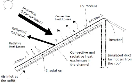
Fig. 2.6. Schematic of a BIPV/T applied on a roof [6]

Over the last few years, several customized mathematical models have been developed for these systems. Chen et al. (2010) [43], Candanedo et al. (2010) [6] and Pantic et al. (2010) [44] modeled and designed a forced ventilated BIPV/T system installed on the roof of a demonstration house. Shahsavar et al. (2011) [45] analyzed energy savings in buildings that use BIPV/T roof systems for interior room air heating. Vats et al. (2012) [46–48] performed an analysis of energy,

Chapter 2 / Approach

exergy and the packing factor of a semi-transparent ventilated BIPV/T system. Fig. 2.6 shows an example of a BIPV/T system installed on roof.

Yin et al. (2013) [49] designed and studied the performance of a completed system of a water based BIPV/T installed on a roof with interior room storage. The substrate of the panel was designed to be integrated into the building skin, allowing the panel to serve as both structural sheathing and waterproofing. This eliminates the material redundancies of current industry standard designs and the embodied carbon associated with those materials. The integration of the panel into the building skin also eliminates the waterproofing problems associated with the roof penetrations required to mount conventional panels on a sloped surface.

Fig. 2.7. a) Schematic of a water based BIPV/T applied on a roof, b) Schematic of a water based PV/T [49]

2.3. A

Experimental and numerical approaches have been used to explore PV building integration, its design and performance. In 1999, Krauter et al. [9] conducted an experimental study for a BIPV/T system. Other authors have developed numerical work for various BIPV/T systems [24,26,38,48].

Authors seem to favor a combination of numerical and experimental approaches. Depending on the level of detail and the parameters studied, the heat transfer across these systems can be modeled using a simple thermal network model to a more complex, Computational Fluid Dynamics (CFD). Fig. 2.8 shows an example of a thermal network.

The simpler models that use a thermal network approach (Fig. 2.8) tend to use standard programming software. Athienitis et al. (2005) [33] used Matlab® to implement a double facade for pre-heating fresh air, generating electricity with integrated photovoltaic panels and storing solar energy in phase-change material. A simple transient numerical control volume model is developed for the heat transfer in the PCM.

Fig. 2.8. Example of a thermal network of a BIPV/T roof system [6].

This type of approach allows the application of different configurations. In this same work, different types of facade systems were studied with computer simulations and full scale experiments. Matlab® was also used by Agrawal and Tiwari (2010) [40] to evaluate the performance and compute the useful exergy for four combinations of the BIPVT systems, i.e. case 1–case 4, at constant mass flow rate and constant velocity of air. The authors used the same software to evaluate the efficiency and life cycle cost of the above BIPV/T system. Candanedo et al. (2010) developed two thermal models for the same system – Steady State Model and Transient Model - both were conceived in Matlab®. This software includes interfaces for dynamic systems simulations, such as Simulink®. Aelenei et al. (2013) [36,37] used Simulink® to implement a model of a BIPV/T-PCM. This model included a physic mode simulation with Simscape® library.

For a more complex approach, some authors resort to computer simulation with CFD techniques for different BIPV/T systems. The CFD simulation solves the Reynolds Average Navier-Stokes form of the governing partial differential equations for fluid flow and heat transfer with a finite volume method. Corbin and Zhai (2010) [42] used CFD simulation on the basis of the experimental tests. Koyunbaba et al. (2011) also used this approach to model a BIPV Trombe wall. A study of energy efficiency and ventilation performance of a ventilated BIPV wall was performed by Lin et al (2011) [28]. This type of software contains the broad physical modeling capabilities needed to model the flow, turbulence, heat transfer, and reactions of many systems. Ghani et al (2012) [17] studied the effect of distribution on the PV performance of a BIPV/T collector using a CFD simulation program, Multi Physics Comsol®. A three step numerical analysis was conducted to model flow distribution, temperature variation, and photovoltaic yield for a PV/T collector whose design, geometric shape, and operating characteristics varied in order to vary flow uniformity within the collector. ANSYS Fluent® and TRNSYS® are also widely used to find out the impact of wind flow around the collector and to study different shapes of collector. These simulations are capable of providing very useful and accurate information, if accurate

Chapter 2 / Efficiency

boundary layer conditions are provided. TRNSYS is basically used by researchers to study the overall performance of systems and for parametric analysis [50]. Kim and Kim (2012) [27] used TRNSYS for modeling an air-type building integrated photovoltaic-thermal system and it was also used by Kalougirou (2001) [51] for modeling a hybrid PV-thermal solar system. Thevenard (2005) [52] used ESP-r, which proved very useful for estimating the electrical and thermal impact of building integrated photovoltaics. These studies vary from the test room facilities [33] to studies of large scale applications [6].

Fig. 2.9. Example of a CFD simulation flow pattern (left). Example of a CFD simulation PV temperature (right) [28].

2.4. E

Researchers strive to improve the energy efficiency of systems, since some energy is lost in each of the conversion processes. More complex systems that have many components are typically less efficient than simple systems. This is no different for BIPV/T systems. The aim is to make such systems as simple as possible, and as efficient as possible. Making systems that include energy conversions more efficient can help to reduce energy consumption and the production of greenhouse gas emissions. Parameters such as solar radiation and airflow rate, wind velocity, orientation, location, exterior temperature, slope, and material proprieties are particularly important.

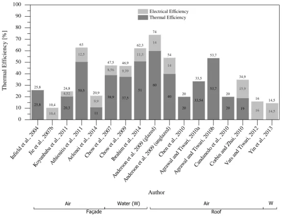
There does seem to be a direct relation between the higher efficiencies obtained by the authors and the type of systems studied (facade, roof, air or water) (Fig. 2.10). Efficiencies of integrated systems in the roof have higher values than those integrated in the facade.

Applications in facades with air as working fluid achieved overall system efficiency between 20.9% and 63% (Jie et al. (2007) presented only the electrical efficiency). Athienitis et al. (2011) [31] demonstrated a high maximum efficiency (63%) system with 50.5% thermal efficiency and 12.5% electrical efficiency. The study was conducted with full-scale prototypes made specifically

for this purpose, including custom PV modules. Other authors showed efficiency values considered normal for such systems [23,24,37]. Looking at integrated systems in facades, we can see that systems with water as the working fluid had higher efficiency (47.5% – 62.3%) than those with air as the working fluid. However, there are too few published papers to establish a rule. Ibrahim et al. (2014) [19] achieved a total maximum efficiency of about 62.3% with 51% thermal and 11.35% electrical, for a spiral flow absorber of water based BIPV/T system.

Fig. 2.10. Graphical summary of the efficiency obtained by the authors.

In Fig. 2.10 we can see that the roof applications have mainly had air as the working fluid. The maximum total efficiencies vary between 14.5% and 74%, for authors who only reported thermal or electrical efficiency. The total maximum efficiency presented by authors is generally greater than the efficiency of systems integrated in the facade. These results are best explained by the slope of the roof relative to the sun. Anderson et al. (2009) [39] presented a study of an unglazed BIPV/T solar collector performance with an overall maximum efficiency of 74%, where 60% is thermal and 14% is electrical efficiency. In the same study, the author described a glazed BIPV/T system with an overall maximum efficiency of 54%, (40% thermal, 14% electrical).

25,8 20,3 50,5 11 38,9 37,5 51 60 40 20 33,54 53,7 20 19 10,4 4,52 12,5 9,9 8,56 9,39 11,3 14 14 15,9 16 14,5 25,8 10,4 24,8 63 20,9 47,5 46,9 62,3 74 54 20 33,5 53,7 20 34,9 16 _14,5 Infie ld e t al., 2004 Jie e t al., 2007b Koy unba ba e t al., 2011 Ath ienit is e t al., 2011 Aele nei e t al., 2014 Cho w e t al., 2007 Cho w e t al., 2009 Ibra him et a l., 2014 Ande rson et a l. 2009 ( glaze d) Ande rson et a l. 2009 ( ungla zed) Che n et a l., 2010 Agr awal a nd T iwar i, 2010a Agr awal a nd T iwar i, 2010b Can dane do e t al., 2010 Cor bin and Z hai, 2010 Vats and T iwar i, 2012 Yin et a l., 2013 0 10 20 30 40 50 60 70 80 90 100 Roof Façade W Water (W) Air T h e rm a l E ff ic ie n c y [ % ] Author Electrical Efficiency Thermal Efficiency Air

B

ASIC

F

UNDAMENTALS OF

H

EAT AND

M

ASS

Chapter 3.

T

RANSFER

3.1. I

The basic fundamentals of heat and mass transfer used to solve the heat transfer phenomena’s across the system is described in this sub-chapter. The conduction, convection and radiation heat transfer modes considered in this study are first briefly reviewed. Then a description of the thermal mass concept is presented. This sub-chapter ends with reference to the phase-change material notion and its numerical approaches.

3.2. H

T

In physics, the heat transfer or propagation is the transition of thermal energy from a warmer to a cooler mass. In other words, it is the exchange of heat energy between two systems of different temperatures.

The energy, called thermal energy in this case, mainly passes from one body to another in three ways: conduction, convection and radiation. These three modes of heat transfer will be described

separately, but in most cases they occur simultaneously. Conduction is the transfer of energy between adjacent bodies or adjacent parts of a body. Convection is the transfer of energy between a body and its environment, due to fluid motion. Radiation is the transfer of energy to or from a body by means of the emission or absorption of electromagnetic radiation.

Consider the very simple system shown schematically in Fig. 3.1 consisting of two bodies with an air gap (either open or closed) between them.

Assuming that there is a temperature difference between the outer (Te) and inner (Ti) boundary

environments, the three heat transfer phenomena mentioned above - conduction, convection and radiation - will occur. In fact, in the two system components, which are solid elements, the heat transfer takes place by conduction only, while in the air cavity the three heat transfer phenomena can coexist.

Finally, regarding the surfaces that are in contact with indoor or outdoor environments, the phenomena of thermal radiation to the surrounding surfaces and convection with the adjacent air in motion will occur. All these phenomena will be described.

Fig. 3.1. Heat transfer through a ventilated air cavity wall system [53]

3.2.1. Conduction Heat Transfer

Heat transfer by conduction is a process that takes place in the presence of temperature differences between two points of a body. This exchange of energy takes place from the region of higher temperature to the lower temperature region by kinetic motion or the direct impact of molecules and atoms [54]. This phenomenon is governed by Fourier’s law, which states that the flow of heat by conduction in a specific direction is proportional to the normal direction, to the

C o nv e ct io n + R adi at io n C o nv e ct io n + R adi at io n C o nv e ct io n + C o nduc ti o n + R ad ia ti o n C o nduc ti o n C o nduc ti o n Ti Te

Chapter 3 / Heat Transfer

direction of flow and to the temperature gradient in this direction. For the one-dimensional plane wall show in Fig. 3.2, having a temperature distribution T(x), the rate equation is expressed as:

'' x T x q  k  (3.1)

where the heat flux q’’x (W/m

2

) is the heat transfer rate in the x direction per unit area perpendicular to the direction of transfer, and it is proportional to the temperature gradient, ∂T/∂x in this direction, and the proportionality constant k is a transport property known as the material thermal conductivity (W/m.K). Under the steady-state conditions (Fig. 3.2), with linear temperature distribution, the temperature gradient may be expressed as:

2 1 T T T x L   _  (3.2) then, 2 1 1 2 x T T T T T q k k k L L L         (3.3)

The heat rate by conduction, qx (W), through a plane wall of area A (m

2

) is the product of the flux and the area:

'' 2 1 1 2 x x T T T T T k A kA kA L L q L q  A      (3.4)

3.2.2. Convection Heat Transfer

The fluid flow at a given temperature over a solid body at a different temperature causes a transfer of heat that is known as surface convection (Fig. 3.3). In general, this heat transfer can be described by Newton's law:

c c

q   h T (3.5)

where q’’, the convective heat flux (W/m2), is proportional to the difference between the surface and fluid temperatures ΔT, and hc is the local convective heat transfer coefficient (W/m

2

K). The heat rate by convection q (W), is the product of the convective heat flux q’’ and the transfer surface area A (m2):

c c

q  q A (3.6)

Fig. 3.3. Boundary layer development in convection heat transfer [55]

Given the wide variability of possible values of h, it is more practical and rational from the scientific point of view for this magnitude to depend on dimensionless parameters.

3.2.2.1. Heat transfer dimensionless numbers

Several dimensionless parameters used to characterize the phenomenon of convection are described in literature. The physical meaning of the dimensionless parameters used in this work to study the phenomenon of convection is described next. These parameters are the Reynolds (Re), Prandtl (Pr), Grashof (Gr), Rayleigh (Ra) and Nusselt (Nu) numbers.

Chapter 3 / Heat Transfer

Reynolds number

The Reynolds number represents the ratio between inertia forces and viscous forces:

2 2 / / Inertia forces V V V Re Viscosity forces V v         (3.7)

Where ρ is the specific mass of the fluid (kg/m3), V is the average velocity (m/s), l is the characteristic length [m] and μ and ν are, respectively, the dynamic (N.s/m2

) and kinematic (m2/s) viscosity of the fluid.

As the Reynolds number increases, the inertia forces become dominant relative to the viscosity, the velocity and pressure fluctuations increase, and the flow may change from laminar to turbulent. Some authors [54] describe a critical Reynolds number where this transition occur. This value depends strongly on the surface roughness and the level of turbulence flow. The characteristic length l, depends on the geometry of the problem. If the flow is over isolated plates, the characteristic length is the distance from the leading edge of the plate, if flow is in ducts, the length is the value of the hydraulic diameter ( Dh ) of the duct , which is defined as:

4 _c h r D A P  (3.8)

where the Acr is the cross-sectional area (m

2

) and P is the wetted perimeter.

Prandtl number

The Prandtl number is the ratio between the momentum diffusivity (kinematic viscosity) and the thermal diffusivity:

p t f C v Pr k     (3.9)

where, μ, Kf and Cp are the dynamic viscosity [N.s/m2], the thermal conductivity (W/m.K) and

Grashof number

The Grashof number represents the relationship between forcing forces and restraining forces; it has a similar role for natural convection as the Reynolds number has for forced convection:

3 2 2 g Δ = Buoyancy Forces g V T Gr Viscous Forces v v       (3.10)

Where g is the gravitational constant (m/s2), β ≅ ∆ρ/(ρ∆T) is the volumetric coefficient of expansion, Pr is the Prandtl number, l is the characteristic length [m] (gap between two layers), ν is the kinematic viscosity (m2/s) and ∆T is the temperature difference between two layers.

As in forced convection with the Reynolds number, in naturally occurring convection there is also a critical Grashof number for which the fluid ceases to have laminar characteristics and changes to a turbulent regime.

Rayleigh number

The Rayleigh number is a dimensionless characteristic parameter of the phenomenon of heat transfer in a fluid and has relative importance for the phenomena of conduction and convection. Conduction is the dominant phenomenon of transfer for Rayleigh numbers of less than a certain critical value of the specific fluid, and convection is the prevailing phenomenon for Rayleigh numbers greater than this value.

The Rayleigh number is the product of the Grashof number and the Prandtl number:

3 2 Δ g Pr Ra PrGr T v    (3.11)

where g is the gravitational constant (m/s2), β is the volumetric coefficient of expansion, Pr is the Prandtl number, l is the characteristic length (m), ν is the kinematic viscosity (m2/s) and ∆T is the temperature difference between two layers.

Nusselt number

The Nusselt number represents the ratio of the actual flow of heat that occurs between a surface and the adjacent fluid, and the heat flow that would occur if the heat transfer was purely by conduction:

Chapter 3 / Heat Transfer Δ Δ / Δ / c c f f f h T h q Nu k T k T k    (3.12)

where q is the flux density at the surface (W/m2), ∆T is the temperature difference between the surface and the fluid (K), hc is the superficial convective heat transfer coefficient (W/m

2

K), Kf is

the thermal conductivity of the fluid (W/m.K), and l is the characteristic length (m).

The Nusselt number may also be viewed as a dimensionless temperature gradient in the boundary layer very close to the solid surface area. Higher Nusselt numbers mean that the heat exchanges are enhanced by convection.

The Nusselt number is expressed in terms of dimensionless parameters which vary according to the nature of the flow (Table 3.1). In a forced convection flow, the Nusselt number is usually a function of the Reynolds number and Prandtl number, while in natural convection it depends on the Rayleigh number. Finally, in mixed convection flows, the Nusselt number is expressed as a function of both the Reynolds and Rayleigh numbers.

Table 3.1. Nusselt number relations depending on the nature of the flow Natural Convection Forced Convection Mixed Convection Nu = f(Ra) Nu = f(Re, Pr) Nu = f(Re, Ra)

The literature reports the use of relations of this kind to characterize the phenomenon of convection in the air cavity that can be used in the numerical model of this work to estimate the value of the surface thermal conductance convection, hc (W/m

2

K), by the following equation:

f c

Nu k

h  (3.13)

Where hc is the superficial convective heat transfer coefficient (W/m

2

K), Nu is the Nusselt number, kf is the thermal conductivity of the fluid (W/m.K) and l is the characteristic length (m).

3.2.3. Radiation Heat Transfer

All bodies emit and absorb electromagnetic radiation at different wavelengths, whose intensity is a function of the absolute temperature and type of surface. Unlike the heat transfer phenomena described above, heat radiation needs no medium or support material to be processed [55].

Despite a PV module is opaque to infrared radiation, there is flux through the longwave radiation absorption and re-emission process. Solar radiation (short wave) is transmitted, reflected

and absorbed in each layer, depending on the optical properties of each element. In this type of study, where the first layer is completely opaque, it makes sense only to study the transfer of heat by radiation of long wave, where are determined the radioactive liquid fluxes of longwave that emit from each surface to its adjacent.

3.2.3.1. Long Wave Thermal Radiation

The law that governs the amount of power radiated from a pure radiant body, commonly termed a black body, at absolute temperature Ts (K), is called the Stefan-Boltzmann law and is expressed

by:

4

b s

E T (3.14)

where σ is the Stefan-Boltzmann constant (σ = 5.67 × 10-8

W/m2.K4) and Eb is the radiation flux

emitted by the black body per unit area (W/m2), which integrates the entire range of lengths wave emission spectra [55].

The heat flux emitted by a real surface is less than that of a blackbody at the same temperature and is given by:

4

s

ET (3.15)

where ε is a radiative property of the surface termed the emissivity. With values in range 0 ≤ ε ≥ 1, this property provides a measure of how efficiently a surface emits energy relative to a blackbody. It depends strongly on the surface material and finish.

Chapter 3 / Heat Transfer

If the surface is assumed to be considered a gray surface (Fig. 3.4), the net rate of radiation heat transfer from the surface, expressed per unit area (W/m2) of the surface, is:





rad s sur

q  T T (3.16)

where Ts is a small surface temperature (K), Tsur is a bigger surrounding surface temperature

(K). The rate of heat transfer by radiation from one surface can be expressed by:





rad s sur

q A T T (3.17)

As can be seen from equation (3.17), the rate of radiative heat transfer between surfaces depends on the difference of the fourth power of the surface temperatures. In many engineering calculations, however, the heat transfer equations are linearized in terms of the differences of temperatures to the first power. For this purpose, the following mathematical identity is considered:

















4 4 2 2 2 2 2 2

s sur s sur s sur s sur s sur s sur

T T  T T T T  T T T T T T (3.18)

Therefore, equation (3.17) can be written as:





rad r s sur

q h A T T (3.19)

Where hr is the radiation heat transfer coefficient modeled in a manner similar to convection.

The radiation rate equation was linearized, making proportional to temperature difference rather than to the difference between two temperatures to fourth power. Note however, that hr depends

strongly on temperature, while the temperature dependence of convection heat transfer coefficient

hc is generally weak. This radiation heat transfer coefficient hr considers not ony the temperature

of the surfaces and their characteristic but also their geometric orientation with respect to each other. The effects of the geometry of radiant energy exchange can be analyzed conveniently by defining the term view factor, F12, to be the fraction of radiation leaving surface A1 that reaches

3.2.3.2. Sky radiation

It is necessary to evaluate the radiation exchange between a surface and the sky. The sky can be considered as a black body at some equivalent sky temperature Tsky so that the actual net radiation

between a horizontal flat plate and the sky is given by equation (3.19). The net radiation from a surface with emittance ε and temperature T to the sky at Tsky is:





rad sky

q  A T T (3.20)

The equivalent black body sky temperature of equation (3.20) accounts for the facts that the atmosphere is not at a uniform temperature and it radiates only in certain wavelength bands. The atmosphere is essentially transparent in wavelength region from 8 to 14 µm, but outside of this “window” the atmosphere has absorbing bands covering much of the infrared spectrum. Several relations have been proposed to relate Tsky for clear skies to measured meteorological variables.

Duffie and Beckman [56] relate a relation for Tsky, where it is used an extensive data set from the

United States to relate the effective sky temperature to the dew point temperature, dry bulb temperature, and hour from midnight t by the following equation:

 

2

0.711 0.0056 0.000073 0.013 cos 15

sky a dp dp

T T _  T  T  t _ (3.21)

where Ta is the dry bulb temperature (K), Tdp is the dew point temperature (ºC). The used

experimental data, covered a dew point range from -20 ºC to 30 ºC. The temperature between sky and air temperatures ranges from 5ºC in a hot, moist climate to 30 ºC in a cold, dry climate.

3.3. T

R

There exists an analogy between the diffusion of heat and electrical charge. Just as an electrical resistance is associated with the conduction of electricity, a thermal resistance may be associated with the conduction of heat. Defining a resistance as the ratio of a driving potential to the corresponding transfer rate, it follows from equation (3.4) that the thermal resistance for conduction in a plane wall is:

1 2 , t cond x T T L R q kA    (3.22)

Chapter 3 / Enthalpy transport

A thermal resistance may also be associated with heat transfer by convection at a surface. From equation (3.6) the thermal resistance for convection is then:

, 1 s t conv c T T R q hA     (3.23)

From equation (3.19) it follows that a thermal resistance for radiation may be defined as:

,rad 1 s sur t rad r T T R q h A    (3.24)

3.4. E

Phenomena of heat transfer also occur between nodes inside the air cavity, and these have to be accounted for. There is a transport of energy by air (enthalpy transport) in the direction of flow, and the net balance between two sections can be calculated by the following expression [57]:





V p in out

q C m T T (3.25)

where qv is the resultant heat flow (W), Cp is the specific heat of air (J/kg K), m is the mass

flow between the nodes (kg /s), and Tin and Tout (K) are, respectively, the temperatures of the fluid

at the inlet and outlet nodes of the air cavity. It is considered that in this model the flow rate is high enough for the phenomena of conduction in the flow direction to be disregarded.

3.5. T

M

A simple transient heat transfer problem is one for which a component experiences a sudden change in its thermal environment. A system’s thermal capacitance is the effective heat capacity of a structure per unit change of interior temperature, and it is important in a system that undergoes significant temperature changes. Thermal capacitance is of particular significance in passive heating or hybrid systems where storage is provided by the system itself. Thermal mass reflects the ability of a material or a combination of materials to store internal energy. The property is characterized by the mass of the material and its specific heat. The equation relating thermal energy q, to thermal mass is [55]: