Application of Superconducting Bulks and Stacks of Tapes in Electrical Machines

(1)

Jorge Manuel Marques Silva

Licenciado em Ciências da

Engenharia Eletrotécnica e de Computadores

Application of Superconducting Bulks and

Stacks of Tapes in Electrical Machines

Dissertação para obtenção do Grau de Mestre em

Engenharia Eletrotécnica e de Computadores

Orientador: João Miguel Murta Pina, Professor Auxiliar, FCT-UNL

Co-orientador: Xavier Granados García, Cientista Titular, ICMAB

Júri:

Presidente: João Almeida das Rosas, Professor

Auxiliar, FCT-UNL

Arguente: Anabela Monteiro Gonçalves Pronto,

Professora Auxiliar, FCT-UNL

Vogal: João Miguel Murta Pina, Professor

(2)

(3)

iii

Application of Superconducting Bulks and Stacks of Tapes in Electrical

Ma-chines

Copyright © Jorge Manuel Marques Silva, Faculdade de Ciências e Tecnologia,

Universidade Nova de Lisboa.

(4)

(5)

À minha Mãe e ao meu Pai.

(6)

(7)

Acknowledgements

At this moment, when presenting this thesis for evaluation by the distinct

members of the jury, it is my duty to express my gratitude to Faculdade de

Ciências e Tecnologia of Universidade Nova de Lisboa (FCT-UNL) and to the

teachers who, have provided me with knowledge over the last five years,

there-fore contributing to my development as a young man in training and a student

in the Integrated Master in Electrical and Computer Engineering (MIEEC).

Throughout this academic journey, I had the opportunity to enjoy two

in-termediate stays during the Master: the first under the Erasmus Study

Pro-gramme in Technische Universiteit Delft (TU Delft) in the Netherlands, for five

months during 2013; and the second under the Erasmus Traineeship

Pro-gramme, a six month stay, during the first semester of the academic year

2014/2015, at Institut de Ciència de Materials de Barcelona (ICMAB) in Spain,

where this dissertation was developed. If during the first stay in Delft, the

sup-port in the application and preparation by the Master coordinator, Professora

Maria Helena Fino, and Lodging and Mobility Office employees, Gracinda

Cae-tano and Ana Dallot, were precious and fundamental, in Barcelona I could

count on the monitoring of my co-supervisor Dr. Xavier Granados as well, to

whom I express my acknowledgment.

Apart from these two enriching experiences, I would like to register my

participation as a monitor in the course of Electrical Circuits Theory, a very

re-warding experience for me and, I hope, useful for my younger colleagues,

whose recognition together with the confidence placed by the course

coordina-tor, Professora Maria Helena Fino, have very positively marked me.

To Professor João Murta Pina, whom I express my gratitude for providing

me the opportunity to experience this internship in Barcelona, where I got the

chance to have a close contact with the laboratory environment, and also for

monitoring my work, especially in this final phase.

(8)

Application of Superconducting Bulks and Stacks of Tapes in Electrical Machines

viii

in Delft, including Giulio and Pablo, and more recently in Barcelona: Thomas,

Joanna, Filip, Pien, Kyra, Tomás, Ana, Joana, Alexa and other members of

Hakuna Party Matata group



.

(9)

Abstract

The present dissertation focuses on the research of the recent approach of

innovative high-temperature superconducting stacked tapes in electrical

ma-chines applications, taking into account their potential benefits as an alternative

for the massive superconducting bulks, mainly related with geometric and

me-chanical flexibility.

This work was developed in collaboration with Institut de Ciència de

Ma-terials de Barcelona (ICMAB), and is related with evaluation of electrical and

magnetic properties of the mentioned superconducting materials, namely:

analysis of magnetization of a bulk sample through simulations carried out in

the finite elements COMSOL software; measurement of superconducting tape

resistivity at liquid nitrogen and room temperatures; and, finally, development

and testing of a frequency controlled superconducting motor with rotor built by

superconducting tapes.

In the superconducting state, results showed a critical current density of

140.3 MA/m

2

(or current of 51.15 A) on the tape and a 1 N∙m developed motor

torque, independent from the rotor position angle, typical in hysteresis motors.

(10)

(11)

Resumo

A presente dissertação foca-se na pesquisa da recente abordagem das

inovadoras fitas supercondutoras de alta temperatura (dispostas em pilha) em

aplicações de máquinas elétricas, tendo em conta os seus potenciais benefícios

como uma alternativa aos blocos supercondutores maciços, principalmente

re-lacionados com a flexibilidade geométrica e mecânica.

Este trabalho foi desenvolvido em colaboração com o Institut de Ciència

de Materials de Barcelona (ICMAB), e está relacionado com a avaliação de

pro-priedades elétricas e magnéticas dos materiais supercondutores mencionados, a

saber: análise da magnetização de um bloco através de simulações realizadas no

software

de elementos finitos COMSOL; medição da resistividade da fita

super-condutora às temperaturas ambiente e do azoto líquido; e, finalmente, o

desen-volvimento e teste de um motor supercondutor controlado por frequência com

rotor construído por fitas supercondutoras.

No estado supercondutor, os resultados mostraram uma densidade de

corrente crítica de 140,3 MA/m

2

_{(ou corrente de 51,15 A) na fita e um binário de 1}

N∙m no motor, independente do ângulo do rotor, típico em motores de histerese.

(12)

(13)

Symbology and Notations

𝑎

Half thickness of the superconducting slab [m].

𝑏

Half length region with no magnetic induction [m].

𝐵

Flux density or magnetic induction field [T].

𝑩

Flux density spatial vector [T].

〈𝑩〉

Average flux density spatial vector [T].

𝐵

𝑎𝑝

Applied flux density [T].

𝐵

𝑚𝑎𝑥

Maximum flux density [T].

𝐵

𝑚𝑎𝑥𝑡𝑢𝑏𝑒

Maximum flux density using a steel tube [T].

𝐵

𝑝

Flux density of penetration [T].

𝐵

𝑥

,

𝐵

𝑦

and

𝐵

𝑧

Flux density spatial components [T].

𝑑

𝑤ℎ𝑒𝑒𝑙

Wheel diameter [mm].

𝐸

Electrical field [V/m].

𝐸

𝑐

Critical electrical field [V/m].

𝐸

𝑠𝑖𝑙𝑣𝑒𝑟

Electrical field in the silver conductor [V/m].

𝑬

𝒔𝒊𝒍𝒗𝒆𝒓

Electrical field in the silver conductor spatial vector [V/m].

𝐸

𝑌𝐵𝐶𝑂

Electrical field in the YBCO bulk [V/m].

(14)

xiv

𝒆

𝒙

Spatial vector unit along

𝑥

-axis.

𝒆

𝒚

Spatial vector unit along

𝑦

-axis.

𝒆

𝒛

Spatial vector unit along

𝑧

-axis.

𝑓

Frequency [Hz].

𝐹

𝑚𝑜𝑡𝑜𝑟

Motor force applied on the wheel [gf].

𝑓

𝑝

Pinning force density [N/m

3

].

𝒇

𝒑

Pinning force density spatial vector [N/m

3

].

𝑓

𝑝𝑦

Pinning force density spatial

𝑦

-component [N/m

3

].

𝑓

𝑟𝑒𝑓

Reference frequency [Hz].

𝑓

𝑠

Sample frequency [Hz].

𝐻

Magnetic field [A/m].

𝑯

Magnetic field spatial vector [A/m].

𝐻

𝑐

Critical magnetic field [A/m].

𝐻

𝑐1

Lower critical magnetic field [A/m].

𝐻

𝑐2

Upper critical magnetic field [A/m].

𝐻

𝑖𝑟𝑟

Irreversibility magnetic field [A/m].

𝐻

𝑝

Penetration magnetic field [A/m].

𝐼

Current [A].

𝐼

𝑐

Critical current [A].

𝑖

𝑝ℎ𝑎𝑠𝑒

Current on one of the phases [A].

𝐼

𝑝ℎ𝑎𝑠𝑒

Current amplitude on one of the phases [A].

𝐽

Current density [A/m

2

_].

𝑱

Current density spatial vector [A/m

2

_].

𝑱

𝒂𝒑

Applied current density spatial vector [A/m

2

].

(15)

𝐽

𝑚𝑎𝑥

Maximum current density [A/m

2

].

𝐽

𝑥

,

𝐽

𝑦

and

𝐽

𝑧

Current density spatial components [A/m

2

].

𝑘

Proportional ratio [H/m].

𝑙

Length of the COMSOL sample or length of the tape fragment

[mm].

𝑀

Magnetization [A/m].

𝑴

Magnetization spatial vector [A/m].

𝑀

𝑖𝑟𝑟

Irreversible magnetization [A/m].

𝑀

𝑟𝑒𝑣

Reversible magnetization [A/m].

𝑛

Exponent parameter in the resistivity expression.

𝑟

Radius [m].

𝑟

𝑤ℎ𝑒𝑒𝑙

Wheel radius [mm].

Δ𝑅

Resistance of the tape fragment [Ω].

𝑆

Cross section of the tape fragment [µm

2

_].

𝑡

𝑚𝑎𝑥

Instant when the applied current density is at its maximum

[ms].

𝑇

Temperature [K].

𝑇

𝑐

Critical temperature [K].

𝑇

𝑐𝑦𝑐𝑙𝑒

Cycle period [s].

𝑡𝑘

Thickness of the tape [µm].

𝑇

𝑚𝑜𝑡𝑜𝑟

Motor torque [N∙m].

𝑇

𝑠

Sample time [s].

Δ𝑈

Voltage drop on the tape fragment [V].

𝑤

Width of the COMSOL layer or width of the tape fragment

[mm].

𝑤

ℎ

Magnetic energy volumetric density [J/m

3

].

(16)

xvi

𝛿

𝑠𝑡𝑒𝑝

Angle step [°].

𝜇

𝑜

Magnetic permeability in the vacuum [4π×10

-7

H/m].

𝜌

Electrical resistivity in the silver conductor [Ω∙m].

𝜎

Tensile stress [MPa] or electrical conductivity [S/m].

𝜎

𝑡𝑢𝑏𝑒

Tensile stress caused by the steel tube [MPa].

𝜒

𝑚

Magnetic susceptibility.

1G

First generation superconducting tape.

2G

Second generation superconducting tape.

BSCCO

Bismuth Strontium Calcium Copper Oxide.

CMOS

Complementary Metal Oxide Semiconductor.

FC

Field Cooling.

HTS

High Temperature Superconductor.

ICMAB

Institut de Ciència de Materials de Barcelona.

LED

Light Emitting Diode.

LTS

Low Temperature Superconductor.

PIT

Process In Tube.

PWM

Pulse Width Modulation.

(RE)BCO

(Rare Element) Barium Copper Oxide.

RPM

Revolutions Per Minute.

SP

Super Power.

UNEX

Universidad de Extremadura.

YBCO

Yttrium Barium Copper Oxide.

(17)

Content

1. INTRODUCTION ... 1

1.1. M

OTIVATION

... 1

1.2. O

BJECTIVES

... 2

1.3. O

RIGINAL

C

ONTRIBUTIONS

... 3

1.4. D

ISSERTATION

O

RGANIZATION

... 3

2. LITERATURE REVIEW ... 5

2.1. G

ENERAL CONCEPTS OF

S

UPERCONDUCTIVITY

... 5

2.1.1. Definition ... 5

2.1.2. Superconductor Types I and II ... 8

2.1.3. High Temperature Superconductors (HTS) ... 9

2.2. HTS

M

AGNETIZATION

... 10

2.2.1. Bean Critical State Model ...11

2.2.1.1. Zero Field Cooling (ZFC) ... 13

2.2.1.1.1. Low Applied Field ... 13

2.2.1.1.2. High Applied Field ... 15

2.2.1.1.3. Excitation Reversal ... 16

2.2.1.2. Field Cooling (FC) ... 16

2.3. HTS

B

ULKS

... 18

2.3.1. Grain Structure ...18

2.3.2. Mechanical Reinforcements ...19

2.3.2.1. Using Steel Tubes ... 19

2.3.2.2. Using Resin Impregnation ... 20

2.3.1. Flux Density Measurements ...21

(18)

xviii

2.4.1. First Generation (1G) ... 23

2.4.2. Second Generation (2G) ... 24

2.4.3. Potential for Applications ... 25

2.4.4. Flux Density Measurements ... 26

3. COMSOL SIMULATION ... 29

3.1. I

NTRODUCTION

... 29

3.2. S

IMULATION AND

R

ESULTS

... 31

3.2.1. Magnetization Curve ... 31

3.2.2. Flux and Current densities ... 32

4. HTS TAPE RESISTIVITY ... 35

4.1. N

ORMAL

S

TATE

... 36

4.2. S

UPERCONDUCTING

S

TATE

... 37

5. HTS MOTOR ... 39

5.1. S

TRUCTURE

... 39

5.2. A

RDUINO

B

OARD

... 40

5.2.1. Wave Characteristics ... 41

5.2.1. Programming Script ... 42

5.2.2. Test with LEDs ... 42

5.3. I

NVERTER

... 43

5.4. M

OTOR

... 44

5.5. E

XPERIMENT AND

R

ESULTS

... 45

5.5.1. Voltage and Current ... 45

5.5.2. Torque ... 46

6. CONCLUSIONS AND FUTURE WORK ... 49

BIBLIOGRAPHY ... LI

APPENDIXES ... LIII

(19)

List of Figures

FIGURE 2.1–A MAGNET LEVITATING ABOVE A HIGH TEMPERATURE SUPERCONDUCTOR (HTS), COOLED WITH LIQUID NITROGEN.PICTURE SOURCE LINK:

HTTP://UPLOAD.WIKIMEDIA.ORG/WIKIPEDIA/COMMONS/THUMB/5/55/MEISSNER_EFFECT_P1390048.JP G/800PX-MEISSNER_EFFECT_P1390048.JPG. ... 6 FIGURE 2.2–SKIN EFFECT REPRESENTATION IN THE CROSS SECTION OF A WIRE. ... 7

FIGURE 2.3–T-J-H DIAGRAM (MURTA-PINA,2010). ... 7

FIGURE 2.4–TYPE-I SUPERCONDUCTOR.PICTURE SOURCE LINK:

HTTP://EN.THEVA.BIZ/USER/EESY.DE/THEVA.BIZ/DWN/SUPERCONDUCTIVITY.PDF. ... 8 FIGURE 2.5–TYPE-II SUPERCONDUCTOR.PICTURE SOURCE LINK:

HTTP://EN.THEVA.BIZ/USER/EESY.DE/THEVA.BIZ/DWN/SUPERCONDUCTIVITY.PDF. ... 8 FIGURE 2.6_–RESISTANCE COMPARISON OF A HTS, A LTS AND A REGULAR CONDUCTOR AS A FUNCTION OF

TEMPERATURE (SELVAMANICKAM,2014). ... 9

FIGURE 2.7–MAGNETIZATION CURVE OF A TYPE-II SUPERCONDUCTOR (KRABBES ET AL.,2006). ... 10

FIGURE 2.8–IRREVERSIBLE AND REVERSIBLE MAGNETIZATIONS OF A TYPE-II SUPERCONDUCTOR (KRABBES ET AL.,

2006). ... 10

FIGURE 2.9_–SKETCH OF A TYPE-II SUPERCONDUCTING SLAB WITH INFINITE DIMENSIONS ALONG AXIS 𝒙 AND 𝒚. MAGNETIC INDUCTION FIELD APPLIED 𝑩𝒂𝒑 ALONG 𝒛-AXIS (MURTA-PINA,2010). ... 12

FIGURE 2.10–FLUX AND CURRENT DENSITIES ALONG 𝒚-AXIS OF A TYPE-II SUPERCONDUCTOR SLAB, AT HALF (A)

AND AT TOTAL (B) PENETRATION FIELD 𝑩𝒑, ACCORDING TO THE BEAN MODEL (MURTA-PINA,2010). ... 14

FIGURE 2.11–FLUX AND CURRENT DENSITIES ALONG 𝒚-AXIS OF A TYPE-II SUPERCONDUCTOR SLAB, WHEN

APPLYING FIELD HIGHER THAN 𝑯𝒑, ACCORDING TO THE BEAN MODEL (MURTA-PINA,2010). ... 15

(20)

xx

FIGURE 2.13–FLUX AND CURRENT DENSITIESEVOLUTION WHEN A TYPE-II SUPERCONDUCTOR SLAB IS FIRST COOLED IN PRESENCE OF FIELD AND AFTER SUBJECTED TO A ITS PROGRESSIVELY REDUCTION, ACCORDING TO

THE BEAN MODEL (MURTA-PINA,2010). ... 17

FIGURE 2.14–EXAMPLES OF YBCOHTS BULKS. ... 18

FIGURE 2.15–GRAIN BOUNDARIES IN A BULK: A) WITH GRANULAR TEXTURE; B) WITH C-AXIS TEXTURE (KRABBES ET AL.,2006). ... 18

FIGURE 2.16–RELATION BETWEEN MAXIMUM TENSILE STRESS AND MAXIMUM TRAPPED FIELD IN A YBCOHTS BULK SAMPLE, WITH OR WITHOUT REINFORCEMENT BY A STEEL TUBE (KRABBES ET AL.,2006). ... 19

FIGURE 2.17_–DISTRIBUTION OF THE TRAPPED FIELD IN A ACROSS A RESIN-IMPREGNATED HTS BULK, MEASURED AT SEVERAL TEMPERATURES (KRABBES ET AL.,2006). ... 20

FIGURE 2.18_–IDEAL FLUX DENSITY IN A YBCO BULK. ... 21

FIGURE 2.19–MEASURED FLUX DENSITY IN A YBCO BULK.THE MEASUREMENTS WERE EXECUTED AT THE DISTANCE OF 1 MM FROM THE SAMPLE... 21

FIGURE 2.20–MICROGRAPHS OF TWO 1GBSCCO TAPES:(A) MONOFILAMENT;(B) MULTIFILAMENT (CEBALLOS MARTÍNEZ,2011). ... 23

FIGURE 2.21–POWDER IN TUBE (PIT) PROCESS (CEBALLOS MARTÍNEZ,2011). ... 24

FIGURE 2.22_–INTERNAL LAYERS OF A 2G SUPERCONDUCTING TAPE (XIONG ET AL.,2007). ... 25

FIGURE 2.23_–APPLICATIONS FOR SUPERCONDUCTING WIRE (STACK OF HTS TAPES IN THIS CASE) (SELVAMANICKAM,2014). ... 26

FIGURE 2.24–MEASURED FLUX DENSITY IN A SINGLE TAPE.THE MEASUREMENTS WERE EXECUTED AT THE DISTANCE OF 1 MM FROM THE SAMPLE... 26

FIGURE 2.25–MEASURED FLUX DENSITY IN A STACK OF TWO TAPES.THE MEASUREMENTS WERE EXECUTED AT THE DISTANCE OF 1 MM FROM THE SAMPLE... 27

FIGURE 3.1_–2D SAMPLE DESIGNED IN COMSOL. ... 29

FIGURE 3.2–MAGNETIZATION CURVE: RELATION BETWEEN 𝑱(𝒙-AXIS) AND 𝑩(𝒚-AXIS)... 31

FIGURE 3.3–FLUX (ARROWS) AND CURRENT (COLORED AREA) DENSITIES SIMULATED IN THE 2D SAMPLE. ... 32

FIGURE 3.4–FLUX (ARROWS) AND CURRENT (COLORED AREA) DENSITIES SIMULATED IN THE 2D EXTENDED SAMPLE. ... 33

FIGURE 4.1–EQUIVALENT CIRCUIT USED TO MEASURE THE RESISTIVITY OF THE TAPE. ... 35

FIGURE 4.2–2GHTS TAPE SUBMERGED IN LIQUID NITROGEN.PHOTO TAKEN DURING THE EXPERIMENT. ... 36

FIGURE 4.3_–RELATION BETWEEN CURRENT DENSITY (J) AND THE ELECTRICAL FIELD (E) ALONG THE TAPE AT THE NORMAL STATE (NON-SUPERCONDUCTING). ... 37

FIGURE 4.4–RELATION BETWEEN CURRENT DENSITY (J) AND THE ELECTRICAL FIELD (E) ALONG THE TAPE AT THE SUPERCONDUCTING STATE (COOLED WITH LIQUID NITROGEN). ... 38

(21)

FIGURE 5.2–COMPLETE CIRCUIT OF THE HTS MOTOR. ... 40

FIGURE 5.3_–RECTIFIED SINUSOIDAL WAVE CREATED IN ARDUINO. ... 41

FIGURE 5.4_–MENU OF THE CREATED PROGRAMING SCRIPT. ... 42

FIGURE 5.5–CIRCUIT WITH LEDS USED TO TEST THE SCRIPT. ... 42

FIGURE 5.6–INVERTER CIRCUIT FOR ONE PHASE. ... 43

FIGURE 5.7–INVERTER USED IN THE EXPERIMENT: A) VIEW FROM ABOVE WITH THE OPTOCOUPLERS, THE CAPACITORS AND CMOS TRANSISTORS; B) VIEW FROM BELOW WITH THE CIRCUIT CONNECTIONS. ... 44

FIGURE 5.8–MOTOR INTERIOR. ... 44

FIGURE 5.9_–MOTOR ROTOR: BEFORE (A) AND AFTER (B) APPLYING THE STACKS OF 2GHTS TAPES. ... 45

FIGURE 5.10_–VOLTAGE AND CURRENT WAVES MEASURED FROM ONE OF THE PHASES. ... 46

FIGURE 5.11_–SETTING TO THE TORQUE MEASUREMENT: A) MOTOR WITH THE SHAFT CONNECTED TO THE MEASUREMENT WHEEL; B) CONNECTION BETWEEN THE MEASUREMENT WHEEL AND THE DYNAMOMETER; C) CONNECTION IN THE DYNAMOMETER; D) DYNAMOMETER DISPLAY. ... 47

(22)

(23)

List of Tables

TABLE 3.1–2D SAMPLE DIMENSIONS. ... 30

TABLE 4.1–TAPE FRAGMENT CHARACTERISTICS. ... 36

TABLE 5.1_–MOTOR DIMENSIONS: ROTOR RADIUS AND AIR GAP. ... 45

(24)

(25)

1. Introduction

1.1. Motivation

Energy availability is a central issue in contemporary society, together

with other as water and environmental sustainability. The near future will be

marked by the search of new forms of conversion and use of energy. Just

con-sider, for example, the new alternative energies and comparability with the

classic; or the potential conflicts at national and international level on the

pro-duction, transmission and use of energy for realizing the scientific,

technologi-cal and social relevance of this matter.

On the one hand, energy and electric power in particular poses problems

of sustainability in environmental terms, but includes also the economic

com-ponents both for the sustainability of companies and for the citizens’ quality of

life. However, strategies have been developed in order to reduce the collateral

damages in terms of environmental externalities through implementation and

application of clean coal technologies. This issue involves contentions in

eco-nomic terms, i.e., the costs are derived not only from research and development

processes but also from more qualified labor.

Feasible solutions are related with the application of converters,

induct-ances or current limiters, which, although conceptually simple, pose other

prob-lems. Therefore, it is important to characterize and evaluate new ways of

con-verting energy and consider the advantages, disadvantages and shortcomings

(26)

2 of alternative answers around the clean technologies and alternative energy

sources.

Facing these challenges, in particular the gains obtained in the production,

transmission and conversion of energy, the implementation of

superconductivi-ty emerges as relevant solution not only from an environmental point of view

as economic, as becoming less dependent on fossil sources and other classical

sources of energy production.

Finally, it should be noted the advantages in energy distribution for

su-perconductivity, namely to diversify energy sources and avoid problems

caused by short circuits when traditional chains fail to overcome and protect

users. In this sense, superconductivity has the possibility to limit the failures

arising from short circuits. However, the implementation of superconductivity

based technologies is complex and does not have uniform criteria nor universal,

so this will certainly be a strong incentive to motivate the advancement in the

design of tools able to innovate, create and develop superconducting

technolo-gies in energy systems, particularly in the use of High Temperature

Supercon-ducting (HTS) materials, also capable of being cooled by abundant and cheap

liquid nitrogen.

1.2. Objectives

This work aims to achieve the following objectives:



Simulate, in the finite elements COMSOL software, a sample of Yttrium

Barium Copper Oxide (YBCO) HTS bulk, in an effort to observe the flux

and current densities;



Measure and test the resistivity of a Second Generation (2G) HTS tape

in two different states: the normal state (at room temperature) and in

superconducting state (temperatures around 77 K);

(27)

1.3. Original Contributions

The original contributions in this work fall mainly on the construction of

the superconducting motor, where the stacks of 2G HTS tapes were applied in

the rotor, constituting an innovation. Also important to point out is the

devel-opment of the frequency controlled motor part: the computer-motor interface

and the development of an Arduino script that controls the field frequency and

the resulting mechanical motor speed.

1.4. Dissertation Organization

This dissertation is organized in six chapters:



Chapter 1: Introduction – the present chapter of Introduction;



Chapter 2: Literature Review – the literature review on

superconductiv-ity and related general concepts. Here there are defined the two types

of superconductivity and distinguished HTS from Low Temperature

Superconductors (LTS) and from a regular conductor. There is a special

focus on HTS bulks and stacks of tapes, as they are the materials to be

used during the experimented work;



Chapter 3: COMSOL Simulation

– a description of the simulation of a

YBCO HTS bulk, carried out in the finite elements COMSOL software

and some considerations regarding flux and currents densities;



Chapter 4: HTS Tape Resistivity

– a report of the experimented

meas-urement of a 2G HTS tape resistivity in two different states: the normal

state (at room temperature) and in superconducting state (temperatures

around 77 K);



Chapter 5: HTS Motor

– a summary on the development of the

super-conducting motor, including all the constituent parts needed to the

im-plementation. Analysis of the results;

(28)

(29)

2. Literature Review

2.1. General concepts of Superconductivity

2.1.1. Definition

Superconductivity is a phenomenon that occurs in certain materials when

cooled below a critical temperature,

𝑇

_𝑐

. Under this condition, the

superconduc-tor material starts to conduct with zero resistance and expels the magnetic field.

This property of complete exclusion and expulsion of the magnetic field

from the superconductor interior is called the Meissner Effect (Meissner

et al.

,

1933)

1

_{. This magnetic property of the material is known as perfect}

diamag-netism. As long as the applied magnetic field

𝑯

does not exceed a certain

criti-cal value,

𝐻

_𝑐

, there is no magnetic induction inside the superconductor, except

on the surface. The correspondent flux density vector

𝑩

(also called magnetic

induction) is given by

𝑩 = 𝜇

0

(𝑯 + 𝑴)

(2.1)

where

𝑴

is the magnetization of the superconductor. When inside the

super-conductor

𝑩 = 0

, Equation (2.1) becomes

𝑯 = −𝑴 ⟹ 𝑯 = 𝜒

𝑚

𝑴

(2.2)

where

𝜒

_𝑚

is called the magnetic susceptibility. In this case, magnetic field and

magnetization vectors have equal intensity but opposite senses, so

𝜒

_𝑚

= −1

,

1_{Translated reference in (Forrest, 1983).}

(30)

6 confirming the perfect diamagnetism of a superconductor. Magnetization is

fur-ther described in Section 2.2.

The Meissner Effect proved superconductivity to be a thermodynamic

state (Rodríguez, 2013) where there are persistent electric current flows on the

surface of the superconductor, acting to exclude the magnetic field of the

mag-net (Faraday's law of induction). These currents effectively form an

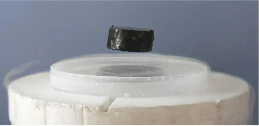
electromag-net that repels the magelectromag-net, as observed in Figure 2.1.

Figure 2.1 – A magnet levitating above a high temperature superconductor (HTS), cooled with liquid nitrogen. Picture source link:

http://upload.wikimedia.org/wikipedia/commons/thumb/5/55/Meissner_effect_p1390048.jpg/ 800px-Meissner_effect_p1390048.jpg.

Even though achieving the critical temperature is fundamental to obtain

the superconductivity state, this is not enough. As previously mentioned,

ex-periments have shown that superconductivity is destroyed for a given upper

threshold of critical magnetic field,

𝐻

_𝑐

. Later, the critical field and temperature

dependence was empirically found (Tinkham, 1996):

𝐻

𝑐

(𝑇) = 𝐻

𝑐

(0) ⋅ [1 − (

_𝑇

𝑇

𝑐

)

2

]

(2.3)

where

𝐻

_𝑐

(0)

represents the field value at the absolute zero temperature (0 K).

Considering a current

𝐼

flowing in a superconducting wire of radius

𝑟

, the

peripheral magnetic field is determined by Ampere's Law (Poole

et al.

, 2007):

𝐻 =

_2𝜋𝑟

𝐼

(2.4)

(31)

𝐼

𝑐

= 2𝜋𝑟 ⋅ 𝐻

𝑐

(2.5)

At the same time, the critical current density in the superconducting wire

𝐽

𝑐

can be calculated. It is important to keep in mind that the current only flows

within a very thin layer at the surface – skin effect – with a penetration depth

𝛿

,

which is significantly smaller than actual radius

𝑟

(

𝛿 ≪ 𝑟

), as portrayed in

Fig-ure 2.2. Consequently,

𝐽

_𝑐

comes (Poole

et al.

, 2007)

𝐽

𝑐

=

_𝜋𝑟

₂

_{− 𝜋(𝑟 − 𝛿)}

𝐼

𝑐 ₂

≈

_{2𝜋𝑟 ⋅ 𝛿 =}

𝐼

𝑐

𝐻

_𝛿

𝑐

(2.6)

Thus, it can be concluded there is also a critical current density

𝐽

_𝑐

, which

also defines whether the material is in superconducting state or not. In

sum-mary, there are three physical quantities that mainly influence the

supercon-ductivity, specifically:



The temperature

𝑇

;



The current density

𝐽

;



The magnetic field

𝐻

(or flux density

𝐵

).

These variables are not independent and they can be represented in

three-dimensional axis, called the T-J-H diagram. The critical values of these variables

form a surface (cf. Figure 2.3) which encloses the necessary conditions for the

material to be supercondutor, i.e. under this surface the material is in the

super-conducting state (Murta-Pina, 2010).

Figure 2.2 – Skin effect

(32)

8

2.1.2. Superconductor Types I and II

Type-I superconductors are elements, in chemical terms. They totally

ex-pel any magnetic field (cf. Figure 2.4), just as stated in Section 2.1.1. As they are

not able to withstand significant fields before they lose superconductivity, these

superconductors are rarely employed (Tinkham, 1996).

Figure 2.4 – Type-I superconductor. Picture source link:

http://en.theva.biz/user/eesy.de/theva.biz/dwn/Superconductivity.pdf.

However, there was discovered a second type of superconductors, which

revealed some penetration of the magnetic field in the form of flux lines (cf.

Figure 2.5), in contrast with type-I. This penetration is a result of the non-pure

sections/zones of these superconductors, for instance, normal conducting

de-fects or degraded superconductivity, where the core of the flux line is pinned,

creating a surrounding vortex of supercurrent. This characteristic allows them

to sustain much higher fields (Murta-Pina, 2010).

(33)

2.1.3. High Temperature Superconductors (HTS)

High Temperature Superconductors (abbreviated HTS) are materials that

behave as superconductors at unusual high temperatures. Whereas "ordinary"

or metallic Low Temperature Superconductors (LTS) usually have transition

temperatures below 30 K (-243.2 °C), HTS have been observed with transition

temperatures as high as 138 K (-135 °C) (Ford

et al.

, 2005).

Most of metal alloys and all HTS are type-II superconductors. In order to

better distinguish the differences between these concepts, a representation of

the observed resistance of a HTS, a LTS and a regular conductor as a function of

temperature is shown in Figure 2.6.

(34)

10

2.2. HTS Magnetization

As previously referred, all HTSs are type-II superconductors. Some of

their basic properties can be described by the field-dependent magnetization.

From Equation (2.1), the magnetization is characterized by

𝑴 =

〈𝑩〉

_𝜇

0

− 𝑯

(2.7)

with

𝑯

as the external magnetic field and

〈𝑩〉

as the average flux density

𝑩

in

the superconductor. The magnetization

versus

field dependence of HTS sample

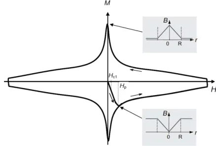
is represented in Figure 2.7.

Figure 2.7 – Magnetization curve of a type-II superconductor (Krabbes et al._{, 2006).}

(35)

In a defect-free type-II superconductor with lower field applied, i.e.

𝐻 < 𝐻

𝑐1

(

𝐻

𝑐1

as the lower critical field), there is a surface current which expels

the external magnetic field so that the magnetic induction

𝐵

in the

supercon-ductor vanishes. As long as the applied field is increased (following the

reversi-ble magnetization line in Figure 2.8), within the range

𝐻

_𝑐₁

< 𝐻 < 𝐻

_𝑐₂

(

𝐻

_𝑐₂

as the

upper critical field), magnetic flux penetrates the superconductor in the form of

flux lines. As the external field increases towards

𝐻

_𝑐₂

, the region between the

flowing flux cores in the superconductor shrinks to zero, and the sample makes

a continuous transition to the normal state. This

𝑀(𝐻)

dependence in the

super-conductor,

𝑀

_𝑟𝑒𝑣

, is reversible and after switching off the external field, no

mag-netic flux is trapped within the superconductor.

The magnetization becomes highly irreversible if the superconductor

in-cludes defects like dislocations, precipitates, etc. These defects interact with the

flux lines and restrains them to penetrate freely at

𝐻 = 𝐻

_𝑐₁

. An applied field

higher than the lower critical field,

𝐻 > 𝐻

_𝑐₁

, the magnetic field starts to

pene-trate the superconductor until reaching the center of the superconductor (at the

penetration field

𝐻

_𝑝

) where the magnetization has its maximum diamagnetic

value. With higher applied fields the magnetization intensity,

|𝑀

_𝑖𝑟𝑟

|

, starts to

decrease (in absolute value), reflecting the reduction of the critical current

den-sity

𝐽

_𝑐

with increasing magnetic field

𝐻

. The irreversible magnetization,

𝑀

_𝑖𝑟𝑟

,

becomes zero at

𝐻 = 𝐻

_𝑖𝑟𝑟

(

𝐻

_𝑖𝑟𝑟

as the irreversibility field) in contrast to the

re-versible magnetization which disappears at

𝐻 = 𝐻

_𝑐₂

. As the external field is

re-duced, the gradient of the local field near the edge changes its sign, but has the

same absolute value as before. The magnetization now becomes positive

be-cause a magnetic field is trapped in the superconductor (Krabbes

et al.

, 2006).

2.2.1. Bean Critical State Model

In the critical state models the distributions of magnetic flux density 𝑩 and

current density

𝑱

, are ruled by the equation

𝑱 × 𝑩 + 𝒇

𝒑

= 0

(2.8)

where

𝒇

_𝒑

is the volumetric density of pinning force in the material.

(36)

Con-Application of Superconducting Bulks and Stacks of Tapes in Electrical Machines

12 sidering that the critical current

𝐽

_𝑐

is either a constant value or zero, from

Equa-tion (2.8), it can be inferred

|𝐽| = 𝐽

𝑐

⟺ 𝑓

𝑝

∝ 𝐵

(2.9)

With the purpose to demonstrate the Bean Model, a superconducting slab

with infinite dimensions along

𝑥

and

𝑧

axes and

2𝑎

of thickness along

𝑦

-axis, as

represented in Figure 2.9, is used as an example. The slab is immersed in an

in-duction field

𝑩

along

𝑧

-axis, defined by

𝑩 = 𝐵

𝑧

𝒆

𝒛

= 𝐵

𝑎𝑝

𝒆

𝒛

(2.10)

Figure 2.9 – Sketch of a type-II superconducting slab with infinite dimensions along axis 𝒙 and 𝒚. Magnetic induction field applied 𝑩_𝒂𝒑 along 𝒛-axis (Murta-Pina, 2010).

Inside the superconducting slab the Ampère’s Law can be verified.

Writ-ing this law in its differential form,

∇ × 𝑯 = 𝑱 ⟺ ∇ × 𝑩 = 𝜇

0

𝑱

(2.11)

where

∇ ×

stands for the curl vector operator. Hence,

∇ × 𝑩 = ||

𝒆

𝒙

𝒆

𝒚

𝒆

𝒛

𝜕

𝜕𝑥

𝜕

𝜕𝑦

𝜕

𝜕𝑧

𝐵

𝑥

𝐵

𝑦

𝐵

𝑧

|| = (

𝜕𝐵

_{𝜕𝑦 −}

𝑧

𝜕𝐵

_{𝜕𝑧 ) 𝒆}

𝑦 𝒙

+ (

𝜕𝐵

_{𝜕𝑧 −}

𝑥

𝜕𝐵

_{𝜕𝑥 ) 𝒆}

𝑧 𝒚

+ (

𝜕𝐵

_{𝜕𝑥 −}

𝑦

𝜕𝐵

_{𝜕𝑦 ) 𝒆}

𝑥 𝒛

(2.12)

Since

𝑩

only has component along

𝑧

,

𝐵

_𝑥

= 𝐵

_𝑦

= 0

, and remembering the

slab is considered to be infinitely long in

𝑥

-axis,

𝐵

_𝑧

is independent from

𝑥

, so

𝜕𝐵

𝑧

𝜕𝑥 = 0

(2.13)

(37)

∇ × 𝑩 =

𝜕𝐵

_{𝜕𝑦 𝒆}

𝑧 𝒙

= 𝜇

0

𝑱 ⟺ 𝑱 = 𝐽

𝑥

(𝑦)𝒆

𝒙

=

_𝜇

1

0

𝜕𝐵

𝑧

𝜕𝑦 𝒆

𝒙

(2.14)

The current density

𝑱

only has component along

𝑥

, given the infinite slab

length along

𝑥

-axis, neglecting

𝐽

_𝑦

. Merging Equations (2.8) and (2.14),

𝒇

𝒑

= −𝑱 × 𝑩 = − |

𝒆

𝒙

𝒆

𝒚

𝒆

𝒛

𝐽

𝑥

(𝑦) 0

0

0 0 𝐵

𝑧

(𝑦)

| = 𝐽

𝑥

(𝑦)𝐵

𝑧

(𝑦)𝒆

𝒚

= 𝑓

𝑝𝑦

(𝑦)𝒆

𝒚

(2.15)

The way the superconductor is magnetized

– Zero Field Cooling (ZFC) or

Field Cooling (FC)

– is undoubtedly relevant, because it leads to different

ef-fects/results. According to (Poole et al., 2007), four different situations may be

considered: low applied field (ZFC); high applied field (ZFC); excitation

rever-sal (ZFC); and finally field applied using FC.

2.2.1.1. Zero Field Cooling (ZFC)

When a superconductor is cooled without applying any field, we are

ob-serving ZFC. If that is the case, the surface currents prevent the penetration of

the applied magnetic field, creating a strong field concentration caused by the

existing diamagnetism (Krabbes

et al.

, 2006).

2.2.1.1.1. Low Applied Field

An initially null external field is progressively applied until there is a full

penetration of the complete field in the superconductor. This means that there

is a central zone totally free of field and current.

Considering the origin of the

𝑦

-axis referential as the center of the slab

along the same axis, as depicted in Figure 2.9, this field-free zone is delimited

by

|𝑦| = 𝑏

, with

𝑏 < 𝑎

. The field starts to penetrate from the borders and

de-creases until becoming zero at

|𝑦| = 𝑏

, so both flux density and current density,

from Equation (2.14), are

𝐵

𝑧

(𝑦) = {𝐵

𝑎𝑝

|𝑦| − 𝑏

𝑎 − 𝑏 , 𝑏 <

|𝑦| ≤ 𝑎

0 ,

|𝑦| ≤ 𝑏

(2.16)

(38)

14 where the function

sgn(𝑦)

returns the sign of the variable

𝑦

(also equivalent to

sgn(𝑦) = 𝑦 |𝑦|

⁄

). Additionally, the critical current density is

−𝐽

𝑐

=

_𝜇

1

0

𝐵

𝑎𝑝

𝑎 − 𝑏 ⟺ 𝑏 = 𝑎 −

𝐵

𝑎𝑝

𝜇

0

𝐽

𝑐

(2.18)

When the increasing applied field equals to the penetrating field

𝐻

_𝑝

(cf.

Figure 2.8), there is no region free of field nor current, because the flux density

𝐵

just reached the center from both sides. This corresponds to the situation

when

𝑏 = 0

. So, from Equation (2.18),

𝑏 = 𝑎 −

𝐵

𝑝

𝜇

0

𝐽

𝑐

= 0 ⟺ 𝐵

𝑝

= 𝜇

0

𝐽

𝑐

𝑎

(2.19)

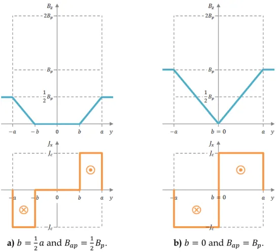
The behavior of both flux density and current density is illustrated in

Fig-ure 2.10, according to the Bean Model, and at two different situations: when

𝑏 =

𝑎₂

and

𝑏 = 0

. The latter is achieving the penetration field

𝐻

_𝑝

(in Figure 2.8),

i.e. the penetration induction field

𝐵

_𝑝

.

a)

𝑏 =

1₂

𝑎

and

𝐵

_𝑎𝑝

=

1₂

𝐵

_𝑝

.

b)

𝑏 = 0

and

𝐵

_𝑎𝑝

= 𝐵

_𝑝

.

(39)

In a ZFC magnetization the trapped field in the sample center remains

ze-ro for applied fields lower than the penetration field,

𝐻 < 𝐻

_𝑝

.

Finally, the pinning force density

𝑓

_𝑝

(𝑦)

results

𝑓

𝑝𝑦

(𝑦) = {𝐽

𝑐

𝐵

𝑎𝑝

|𝑦| − 𝑏

𝑎 − 𝑏 ⋅ sgn

(𝑦) , 𝑏 < |𝑦| ≤ 𝑎

0 ,

|𝑦| ≤ 𝑏

(2.20)

2.2.1.1.2. High Applied Field

Applying field above penetration field

𝐻

_𝑝

, the flux and current densities

and the pinning force density are defined as

𝐵

𝑧

(𝑦) = 𝐵

𝑎𝑝

+ 𝐵

𝑝

|𝑦| − 𝑎

_𝑎

, |𝑦| ≤ 𝑎

(2.21)

𝐽

𝑥

(𝑦) = 𝐽

𝑐

⋅ sgn(𝑦) , |𝑦| ≤ 𝑎

(2.22)

𝑓

𝑝𝑦

(𝑦) = 𝐽

𝑐

(𝐵

𝑎𝑝

+ 𝐵

𝑝

|𝑦| − 𝑎

𝑎 ) ⋅ sgn

(𝑦) , |𝑦| ≤ 𝑎

(2.23)

And the respective graphic representation in Figure 2.11:

(40)

16

2.2.1.1.3. Excitation Reversal

After applying such high field and since the field has reached the center of

the slab, when the excitation is reverted, field and current will vary differently:

Figure 2.12 –Flux and current densitiesevolution when a type-II superconductor slab is sub-jected to a decreasing applied field, according to the Bean Model (Murta-Pina, 2010).

In above Figure 2.12, especially in the last case, further to the right,

alt-hough there is no field at the slab boarders, there is trapped field exactly in the

center, equal to the penetration field

𝐵

_𝑝

. To accomplish this trapped field at the

center it was necessary to externally apply a field twice as higher (cf. Figure

2.11).

2.2.1.2. Field Cooling (FC)

Finally, if the superconductor is cooled under the critical temperature

𝑇

_𝑐

in

presence of a constant magnetic field, the superconductor suffers a stronger

magnetization – larger magnetic susceptibility

𝜒

𝑚

. The superconductor will get

oriented according to the field (Krabbes

et al.

, 2006).

(41)

a)

b)

c)

Figure 2.13 –Flux and current densitiesevolution when a type-II superconductor slab is first cooled in presence of field and after subjected to a its progressively reduction, according to

the Bean Model (Murta-Pina, 2010).

(42)

18

2.3. HTS Bulks

The most used HTS bulks are chemically composed by Yttrium, Barium,

Copper and Oxygen (YBCO) (cf. Figure 2.14), which can handle considerably

high critical current densities at 77 K, and can be used in several applications,

for instance, superconducting magnetic bearings.

Figure 2.14 – Examples of YBCO HTS bulks.

2.3.1. Grain Structure

The orientation of the grains in a HTS bulk is crucial for the current flow.

Randomly oriented grains deprive the current to flow freely due to weaken

bounds between them. This, in turn, limits the flowing currents, disabling any

practical use of the bulk (cf. Figure 2.15a).

These weak bounds can be avoided, granting higher currents, if the HTS

bulk is modified in such a way that grains get aligned in the

c

-axis direction

(perpendicular direction to the

ab-

plane surface of the sample) as seen in Figure

2.15b, using melt-texturing techniques (Krabbes

et al.

, 2006).

a) b)

(43)

The grain structure is easily controlled by applying a magnetic field in

c

-axis and magnetizing by FC. By doing so, the flux lines penetrate effortlessly in

the material and supercurrents are induced in the

ab

plane of the HTS bulk

sample (Krabbes

et al.

, 2006).

2.3.2. Mechanical Reinforcements

One of the drawbacks brought by the HTS bulks is related with

mechani-cal issues, when a very high field is applied. Given the respective low tensile

strength, these materials are not able to withstand such large fields, causing an

eventual material cracking and consequent loss of its diamagnetic properties.

Nevertheless, some approaches can be taken to overcome this problems,

among them, reinforcing the bulk with steel tubes or impregnating resin in its

interior (Krabbes

et al.

, 2006).

2.3.2.1. Using Steel Tubes

In case of using steel tubes, the effect of field enhancement is pictured in

Figure 2.16. The cracking tensile stress is 30 MPa. Without the steel tube, the

tensile stress

𝜎

shows proportionality with the square maximum trapped field

𝐵

𝑚𝑎𝑥2

(Krabbes

et al.

, 2006),

𝜎 ∝ 𝐵

𝑚𝑎𝑥2

⟺ 𝜎 =

_{2𝜇 ⋅ 𝐵}

1

𝑚𝑎𝑥2

⟺ 𝐵

𝑚𝑎𝑥2

= 2𝜇 ⋅ 𝜎

(2.24)

where

𝜇 [H/m]

is the magnetic permeability. In this case, considerable low

trapped fields are capable of cracking the YBCO bulk.

(44)

20 However, if a steel tube is used, a negative, compressive and constant

stress

𝜎

_{𝑡𝑢𝑏𝑒}

acts on the encapsulated YBCO bulk (Krabbes

et al.

, 2006). With

in-creasing trapped field, the bulk tensile stress is steadily counterbalancing this

tube stress until exceeding and finally cracking both bulk and tube. In this other

case, we have

𝜎 =

_{𝑘 ⋅ 𝐵}

1

𝑚𝑎𝑥𝑡𝑢𝑏𝑒2

− |𝜎

𝑡𝑢𝑏𝑒

| ⟺ 𝐵

𝑚𝑎𝑥𝑡𝑢𝑏𝑒2

= 𝑘 ⋅ (𝜎 + |𝜎

𝑡𝑢𝑏𝑒

|)

(2.25)

From Equations (2.24) and (2.25), it is evident

𝐵

𝑚𝑎𝑥𝑡𝑢𝑏𝑒

> 𝐵

𝑚𝑎𝑥

(2.26)

which is also noticeable in the Figure 2.16. The bulk is now more resistant

be-cause it cracks at a much higher trapped field.

2.3.2.2. Using Resin Impregnation

Another solution for the mechanical issue is using impregnating resin in

the bulk interior. Molten resin can be added inside a YBCO bulk, through

mi-crocracks at the surface. In this way, an enhancement of the tensile strength

from 18.4 to 77.4 MPa was achieved (cf. Figure 2.17) (Krabbes

et al.

, 2006).

(45)

2.3.1. Flux Density Measurements

In order to analyze the performance of a YBCO bulk (32 mm × 40 mm × 10

mm), some measurements of trapped flux density were conducted in

Univer-sidad de Extremadura (UNEX) in Badajoz, Spain (Murta-Pina,

et al.

, 2014).

The ideal trapped flux density is represented in Figure 2.18, according to

the Bean Critical State Model (Section 2.2.1) and Figure 2.19 shows the real

measured flux density in the YBCO bulk.

Figure 2.18 – Ideal flux density in a YBCO bulk.

Figure 2.19 – Measured flux density in a YBCO bulk. The measurements were executed at the distance of 1 mm from the sample.

x [mm] y [mm] 0 10 20 30 0 10 20 30 40 0 0.05 0.1 0.15 0.2

Ideal flux density in a bulk

B [ T] 0 0.05 0.1 0.15 0.2 0 10 20 30 0 10 20 30 40 0 0.05 0.1 0.15 0.2

Measured flux density in a bulk

(46)

22 The data related to these graphic representations is detailed in Appendix

1: script_measurements_bulk_tapes.m.

(47)

2.4. HTS Tapes

There is no technology which can currently provide as compact a source

of high magnetic field as magnetized superconducting bulks. When using the

FC method of magnetization, fields over 17 T have been trapped between two

YBCO bulks (Tomita

et al.

, 2003).

However, a significant problem with existing bulks is the thermal

instabil-ity below 30 K (Krabbes

et al.

, 2006) which makes it impossible or impractical to

exploit large

𝐽

_𝑐

values which exist at low temperatures. Besides, the previously

mentioned reasons are also pertinent: the existing superconducting bulks

re-quire external mechanical reinforcement for very high trapped fields, due to the

poor mechanical strength.

In an attempt to overcome the limitations identified in the bulks, a recent

approach on innovative HTS stacked tapes in electrical machines applications is

considered, bringing potential benefits, mainly related with geometric and

me-chanical flexibility. In this regard, a stack of (RE)BCO coated conductor tapes,

(RE stands for a Rare-Earth element) is mechanically stronger due to the

metal-lic substrate supporting the superconducting layer and therefore seems a

natu-ral choice for trapping very high fields.

2.4.1. First Generation (1G)

A first generation (1G) tape consists of one or more filaments of

supercon-ducting powder encased in cylindrical sheaths (silver or silver alloy) (see Figure

2.20). Commonly, the material used in this superconducting powder is Bismuth

Strontium Calcium Copper Oxide (BSCCO). When the material is used as part

of electrical systems, the silver coat provides an alternate path for current when

the superconductor transits to normal (Ceballos Martínez, 2011).

a) b)

(48)

24 To produce this tape, it is used the Powder In Tube (PIT) process,

de-scribed in 3 phases: drawing, rolling and sintering. The drawing process

com-pacts the superconductor powder. Rolling orients the grains with the

ab

planes

parallel to the direction of the tape, favoring supercurrents along it. Finally,

sin-tering provides the superconducting character with continuity (Ceballos

Mar-tínez, 2011). This whole process is illustrated in Figure 2.21.

Figure 2.21 – Powder In Tube (PIT) process (Ceballos Martínez, 2011).

Overall, 1G tapes are not always the best choice because it is made of

ex-pensive materials, requiring an intensive manufacturing labor and reveals

per-formance limitations, especially in high magnetic fields.

2.4.2. Second Generation (2G)

In fact, 2G tapes appeared as an alternative to 1G tapes so that they could

work in environments with magnetic fields stronger than those that the latter

can support, as mentioned above. Therefore 2G tapes are better suited to

elec-trical applications.

(49)

layer provides mechanical stability, by keeping the superconducting layer away

from the surface and increases electrical stability, improving current flow once

the superconducting layer is saturated (Ceballos Martínez, 2011). In brief, the

tape is produced in a continuous reel-to-reel process, only 1% of wire is the

su-perconductor and approximately 97% is inexpensive nickel alloy and copper.

The internal design of a 2G superconducting tape is portrayed in Figure 2.22.

Figure 2.22 – Internal layers of a 2G superconducting tape (Xiong et al._{, 2007).}

By virtue of all the advantages and efficiency brought by the 2G HTS

tapes, they have been used in the respective laboratory experiments for the

pre-sent work. In order to achieve higher trapped fields, several tapes stacked on

top of each other were used, assembling the so-called stack of HTS tapes.

2.4.3. Potential for Applications

The potential of a stack of HTS tapes to be used as trapped field magnets

in different energy applications is very significant. Such samples have relatively

uniform

𝐽

_𝑐

when compared to bulks, resulting in predictable performance.

Some significant benefits of HTS tapes in energy applications are, among others

(Selvamanickam, 2014):



The liquid nitrogen used as coolant is a dielectric medium. Using this

material, the possibility of oil fires and related environmental hazards is

eliminated;

(50)

26 Some examples of possible applications using the superconductor wire

(i.e. stack of tapes) are labeled in the organization chart below, in Figure 2.23.

Figure 2.23 – Applications for superconducting wire (stack of HTS tapes in this case) (Selva-manickam, 2014).

Finally, the cost of superconducting tapes is steadily and predictably

fall-ing, making the technology attractive for engineering applications.

2.4.4. Flux Density Measurements

Besides the YBCO bulk, some experiments were conducted in order to

de-termine the trapped field in 2G HTS tapes (or stack of tapes), in UNEX, Badajoz,

Spain (Murta-Pina,

et al.

, 2014).

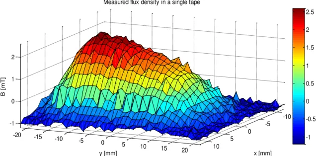
Two experiments were considered: the first measurement with a single

tape (cf. Figure 2.24) and the second using two stacked tapes (cf. Figure 2.25).

Figure 2.24 – Measured flux density in a single tape. The measurements were executed at the distance of 1 mm from the sample.

-10 -5 0 5 10 -20 _-15 -10 _-5 0 ₅ 10 ₁₅ 20 -1 0 1 2 x [mm] Measured flux density in a single tape

B [ m T] -1 -0.5 0 0.5 1 1.5 2 2.5

(51)

Figure 2.25 – Measured flux density in a stack of two tapes. The measurements were executed at the distance of 1 mm from the sample.

The data related to these graphic representations is detailed in Appendix

1: script_measurements_bulk_tapes.m.

In conclusion, when the stack of two tapes is used, rather than a single

tape, the flux density is higher and more uniform, and so is the magnetic field.

In these stacked tapes there is only a

“hill” where the field is maximum,

because the current flows in a single ring, unlike the bulks, where various

do-mains and subdodo-mains are likely to exist, due to the mechanical cracks.

In comparison with the bulk, these two stacked tapes are only able to

ob-tain a maximum field of 3.5 mT, while in the bulk, despite the cracks, it was

possible to achieve 0.2 T. A way to increase the field is placing more tapes in the

stack, as proven in this experiment.

y [mm] x [mm]

-10 -5 0 5 10 -20 _-15

-10 _-5

0 ₅

10 ₁₅ 20 0.5

1 1.5 2 2.5 3 3.5

x [mm] Measured flux density in a stack of two tapes

B

[

m

T]

(52)

(53)

3. COMSOL Simulation

3.1. Introduction

During the progress of the present dissertation, simulations were

per-formed in COMSOL software in order to virtually determine the behavior of a

HTS bulk. The HTS bulk sample (cf. Figure 3.1) was designed in 2D plane,

in-stead of 3D to simplify and save simulation time.

Figure 3.1 – 2D sample designed in COMSOL.

This sample includes four layers: two of liquid nitrogen (used for isolation

purposes), one of silver (as electric conductor) and one of YBCO (the actual

A)

Liquid Nitrogen

B)

Silver (conductor)

C)

Liquid Nitrogen

D)

YBCO

(54)

30 perconductor) with the dimensions of length (l) along

𝑥

-axis and width (w)

along

𝑦

-axis indicated in Table 3.1. Liquid nitrogen was used not only to

pro-vide the temperature condition for the YBCO layer to be in the superconducting

state (around 77 K), but also because it is a better dielectric than air.

Table 3.1 – 2D sample dimensions.

Liquid Nitrogen

Silver

YBCO

w [mm]

4 (layer A)

1 (layer C)

3

1 l [mm]

6 In the silver conductor (layer B) the current

𝑱

_𝒂𝒑

is applied depending on

the time and space in

𝑧

-axis direction, perpendicular with the

𝑥𝑦

-plane, being

𝑱

𝒂𝒑

= 𝐽

𝑎𝑝𝑧

(𝑥, 𝑡)𝒆

𝒛

= 𝐽

𝑚𝑎𝑥

cos (

𝜋𝑥

2𝐿) sin

(2𝜋𝑓𝑡) 𝒆

𝒛

(3.1)

where the maximum current density applied is

𝐽

_𝑚𝑎𝑥

= 500 MA/m

2

, and the

considered frequency is

𝑓 = 1 kHz

.

The induced current density

𝑱

within the entire sample can be obtained

from

Ampère’s Law, in its differential form, remembering

𝑱

only has

compo-nent in

𝑧

-axis. Thus,

𝑱 = 𝐽

𝑧

𝒆

𝒛

= ∇ × 𝑯 = (

𝜕𝐻

_{𝜕𝑥 −}

𝑦

𝜕𝐻

_{𝜕𝑦 ) 𝒆}

𝑥 𝒛

(3.2)

Inside the silver conductor, the electrical field

𝑬

is a result of both applied

and induced current densities

𝑬

𝒔𝒊𝒍𝒗𝒆𝒓

= 𝐸

𝑠𝑖𝑙𝑣𝑒𝑟𝑧

𝒆

𝒛

= 𝜌

(𝑱 + 𝑱

𝒂𝒑

)

(3.3)

where

𝜌

_{𝑠𝑖𝑙𝑣𝑒𝑟}

represents the silver conductor electrical resistivity.

On the other hand, the electrical field in the YBCO bulk in the

supercon-ducting state (around 77 K) is described by

𝑬

𝒀𝑩𝑪𝑶

= 𝐸

𝑌𝐵𝐶𝑂

𝒆

𝒛

= 𝐸

𝑐

⋅ (

_𝐽

𝐽

𝑐

)

𝑛

(3.4)

(55)

tape

– detailed in Section 4.2. In practice, this means the YBCO bulk does not

have significant losses by Joule effect until a critical current density

𝐽

_𝑐

(consid-erably very high), enabling the YBCO bulk to handle high currents.

3.2. Simulation and Results

3.2.1. Magnetization Curve

After simulating, it was intended to observe the magnetization curve that

should be similar to the theoretical curve observed in Section 2.2, Figure 2.7.

From COMSOL, it was possible to retrieve average values of the output

current density

𝑱

(only with component

𝐽

_𝑧

) and output magnetic field

𝑯

(with

components

𝐻

_𝑥

and

𝐻

_𝑦

) on the surface of the superconductor layer (layer D in

Figure 3.1). Considering

the vectors’ lengths absolute values and

the magnetic

permeability in the superconductor to be

𝜇

₀

, the dependence

𝐵(𝐽)

can be

de-termined by

𝐵(𝐽) = 𝜇

0

𝐻(𝐽)

(3.5)

This dependence is represented in Figure 3.2.

(56)

32 The results have shown an absolute maximum value of current density of

280 MA/m

2

_{and a maximum flux density no greater than 400 mT.}

This outcome is different from expected, as the variables are not exactly

the same as in Equation (2.7) and they are being compared from different axes:

𝐽

from

𝑧

-axis and

𝐻

from

𝑥𝑦

-plane, in absolute values. The superconductor

fol-lows a curious hysteresis loop. This question may be analyzed as future work.

3.2.2. Flux and Current densities

The observation of flux and current densities in the simulation sample is

equally significant to understand how the superconductor reacts to an applied

current in the silver conductor. From Equation

(3.1), choosing an instant

𝑡

_𝑚𝑎𝑥

where the current density applied is at its maximum (using

𝑓 = 1 kHz

),

sin(2𝜋𝑓𝑡

𝑚𝑎𝑥

) = 1 ⟺ 𝑡

𝑚𝑎𝑥