Modelling nitrogen emissions from soils fertilized with
dairy slurry
Rick Hao Chen Li
Dissertação para a obtenção do Grau de Mestre em
Engenharia do Ambiente
Orientadores: Professora Maria do Rosário Cameira
Professor David Fangueiro
Júri:
Presidente: Doutor António José Guerreiro de Brito, Professor Associado com Agregação do Instituto Superior de Agronomia da Universidade de Lisboa;
Vogais: Doutora Maria do Rosário da Conceição Cameira, Professora Associada do Instituto Superior de Agronomia da Universidade de Lisboa;
Doutora Cláudia Saramago de Carvalho Marques dos Santos Cordovil, Professora Auxiliar do Instituto Superior de Agronomia da Universidade de Lisboa.
Foremost, I want to express my sincere gratitude towards my advisors’ support and guidance throughout my Master’s thesis, Professor Maria do Rosário Cameira for her patience, motivation and enthusiasm. Modelling can be difficult, and most likely this would not have been possible if not by the continuous encouragement and many hours devoted to the model. Professor David Fangueiro for his patience, motivation and enthusiasm, and for providing field data necessary for this work. To reiterate, I am genuinely thankful for my advisors’ help. I would also like to thank Professor Fernanda Valente, of the Mathematics Department, for her continuous help and guidance regarding not only the statistical part used for the present study, but the thesis in general.
Finally, toward my family, friends and colleagues, I can only express my deepest gratitude for their support, friendship, encouragement and trust which all helped me go through another important phase of my professional and personal life.
Diffuse nitrogen (N) emissions from agriculture have been increasing for the past decades constituting a major environmental problem. Instruments have been implemented during the last years such as legislations, technologies and measures to reduce emissions, but the diversity of the cropping systems allied with the complex diffuse N pathways resulted in an overall inefficiency of these instruments. As such, a holistic approach is needed, being the system modelling one important tool for that.
The Root Zone Water Quality Model was tested for a sandy soil (Haplic Arenosol) and a sandy loam soil (Haplic Cambisol), cultivated with winter oats (Avena Sativa L.) fertilized with dairy slurry. Field data was collected at Horto de Química Agrícola of the Instituto Superior de Agronomia in Lisbon, consisting of soil water, temperatures and drainage from 2014 to 2016. Data from previous studies (2012 to 2014) relative to nitrate leaching and N2O emissions was
also used. The model was then used for scenario analysis.
For the winter oats in the sandy soil, the model predicted soil water and drainage with efficiencies of 86 and 94 % respectively, while for nitrate fluxes below the root zone and the N2O emissions to the atmosphere efficiency was 89 and 93% respectively. For the sandy loam
system, the calibrated model yielded efficiencies of 87, 94, 62, 76 and 85%, for the control variables. Scenario analysis showed the occurrence of pollution swapping as the hydrologic year changed from very dry to wet, decreasing the N lost through gaseous emissions. As to the temperature scenarios results show that for this type of production systems, the most unfavourable climate change scenario was A1B1 (+4ºC) may produce an increase of 25 and 18 % in the N gas loss contributions for the sandy loam and the sandy soil respectively.
Emissões difusas de azoto da agricultura têm vindo a aumentar durante as últimas décadas, sendo um grande problema ambiental. Instrumento, como legislações, tecnologias e medidas de redução foram implementadas para reduzir estas emissões, contudo a grande variabilidade dos sistemas de cultura acoplado à complexidade das vias de emissão difusa do azoto tornaram estes ineficazes. Portanto uma abordagem holística é necessária, onde a modelação de sistemas integrados é uma importante ferramenta.
O Root Zone Water Quality Model foi testado para um solo arenoso (Haplic Arenosol) e um franco arenoso (Haplic Cambisol), cultivado com aveia (Avena Sativa L.) e fertilizado com chorume bovino. Os dados de campo foram recolhidos no Horto de Química Agrícola do Instituto Superior de Agronomia em Lisboa, como o teor de água, temperatura e drenagens de 2014 a 2016. Dados como a lixiviação de nitratos e emissão de N2O de estudos anteriores
também foram utilizados. O modelo foi utilizado para a análise de cenários.
Para o solo arenoso, o modelo previu os teores de água e drenagens com eficiências de 86 e 94% respetivamente, para os fluxos de nitratos abaixo da zona radicular e as emissões de N2O para a atmosfera obteve-se eficiências de 89 e 93% respetivamente. No solo franco
arenoso, o modelo calibrado devolveu eficiências de 87, 94, 62, 76 e 85% para as variáveis de controlo. A análise de cenários mostrou a ocorrência de pollution swapping à medida que o ano hidrológico mudou do muito seco para o húmido, com diminuição do azoto perdido através de emissões gasosas. Resultados dos cenários de temperatura revelam que para este sistema de produção, o cenário de alterações climáticas mais desfavorável é o A1F1 (+4ºC), onde se verificou um aumento de 25 e 18% na contribuição das perdas gasosas de azoto para os solos franco arenoso e arenoso, respetivamente.
PALAVRAS-CHAVES: Modelação de sistemas; RZWQM2; Poluição difusa; Lixiviação de
O azoto é um elemento que é essencial para a vida no planeta Terra, estando presente na constituição das proteínas, e ao mesmo tempo o mais comum no planeta. Embora a vasta maioria do azoto na Terra esteja “armazenado” na atmosfera na forma de gás (N2), que é uma
forma não diretamente assimilável pelas plantas, também se pode encontrar azoto no solo, sedimentos e rochas em formas orgânicas ou inorgânicas, pelo que é o nutriente que mais limita o crescimento vegetal.
Com a intensificação da produção de alimento desde o século XX até a atualidade, em resposta ao crescimento exponencial da população mundial durante o mesmo período, resultou numa intensificação da agricultura, e consequentemente num aumento da produção e utilização de água e fertilizantes a nível global. Este aumento levou a vários problemas ambientais, como a emissão de gases com efeito de estufa, contaminação dos corpos de água com nitratos e nitritos, e outros impactes negativos, em várias regiões do planeta, incluindo na Europa. Atualmente a agricultura é a principal atividade humana responsável poluição ambiental devido às emissões difusas do azoto.
Entretanto, vários instrumentos legais, tecnologias e medidas com o intuito de diminuir as emissões de azoto foram aplicadas e implementadas, mas dado à grande variedade dos sistemas de cultura que em conjunção com a complexidade das vias de emissões difusas do azoto deram origem a medidas reguladoras pouco eficazes para os diferentes tipos de sistemas de produção. Adicionalmente, vários estudos frisam o risco de ocorrer “pollution
swapping” entre as várias vias de emissão do azoto, como por exemplo entre a lixiviação de
nitratos e a emissão de amoníaco. Para se conseguir estudar as emissões difusas do azoto no sistema cultura-solo, é necessário uma abordagem holística desta problemática, incluindo a dinâmica do azoto e as práticas de gestão do azoto nos sistemas integrados cultura-solo-atmosfera.
Uma das ferramentas ideais para seguir este tipo de abordagem é a modelação dos sistemas integrados, onde o modelo consegue conciliar as interações entre os diferentes componentes de um sistema agrícola, pelo que os diferentes processos de transformação e transporte do N que ocorrem nos diversos compartimentos dos sistemas são considerados e relacionados com o regime hídrico do solo. O que foi efetuado no presente trabalho, através da utilização e avaliação do modelo RZWQM2.
O presente trabalho tem como principal objetivo modelar as emissões de azoto a partir de um sistema agrícola com a cultura de aveia, fertilizado com chorume bovino, calibrando e validando o modelo para um solo arenoso e solo franco arenoso com aplicação de chorume bruto com incorporação, assim como fazer uma comparação entre os dois solos, no que
respetivos regimes hídricos e temperaturas. Após finalizada a calibração e validação do modelo, e com este a simular os diversos processos relacionados com a água e azoto nos diversos compartimentos, com a precisão pretendida, utilizou-se o modelo para estimar os balanços de água e azoto, bem como as perdas de azoto para diferentes cenários relacionados com os anos hidrológicos e as alterações climáticas. Também foi efetuada uma simulação para se estimar os fluxos de nitratos lixiviados resultantes dos solos com aplicação de chorume de cinco tratamentos diferentes, com base nas drenagens simuladas e as concentrações medidas de nitratos na solução do solo, tendo sido efetuado a uma análise de variância dos resultados.
Foram instalados cinco lisímetros para cada tipo de solo (arenoso e franco arenoso), um para cada tratamento de chorume, perfazendo um total de dez lisímetros no Horto de Química Agrícola Boaventura Azevedo do Instituto Superior de Agronomia. Em cada lisímetro, colocaram-se aparelhos/equipamentos para medir os teores de água, temperatura, concentrações de nitratos e emissões de N2O, que foram utilizados para o presente estudo.
As medições das drenagens de água a 100 cm de profundidade foram efetuadas a partir de colheitas no interior de um túnel de acesso, diretamente abaixo dos lisímetros. Estas medições decorreram nas épocas húmidas de 2012 a 2016, com as emissões de azoto a serem recolhidas entre 2012 e 2014, enquanto que o teor de água, drenagem e temperatura do solo a serem coletados entre 2014-2016.
O modelo foi calibrado segundo um procedimento iterativo, em que se selecionaram alguns parâmetros sujeitos a serem alterados até o modelo conseguir resultados semelhantes aos medidos em 2014-2015, para as variáveis de controlo teor de água, drenagem, temperatura, emissões de nitratos e amoníaco. Os parâmetros escolhidos foram o teor de água a 10 kPa (capacidade de campo), a condutividade hidráulica saturada, os coeficientes relativos à partição da matéria orgânica e os parâmetros relativos às transformações do N. Sendo posteriormente validado com dados independentes de 2012-2013 2013-2014 e 2015-2016 para as mesmas variáveis.
No final do processo de modelação, o modelo mostrou-se apto a simular os diferentes processos relacionados com a água e azoto no solo com a precisão pretendida, tendo em conta os diferentes resultados para a avaliação da qualidade do modelo, como a eficiência de modelação (EF), que no geral foi elevada para as variáveis consideradas, também o erro médio quadrático (RMSE) foi determinado, com resultados razoáveis. Ambos EF e RMSE resultantes do presente trabalho estão em conformidade com os valores obtidos por outros autores. Verificou-se ainda, que a qualidade de modelação foi melhor para o solo arenoso aquando comparado com o solo franco arenoso.
relacionados com diferentes anos hidrológicos (muito seco, seco, médio e húmido) e de alterações climáticas (aumento da temperatura média em 1.8 ou 4.0 ºC).
No que toca aos cenários dos anos hidrológicos, verificou-se que em média a contribuição da precipitação para a evapotranspiração é 42% superior para o solo franco arenoso do que o solo arenoso, por outro lado a contribuição da precipitação na drenagem é 12.5% menor. Sendo que as maiores diferenças ocorrem nos cenários mais secos enquanto que nos cenários mais húmidos que estes, o aumento na quantidade de precipitação consegue “mascarar “, até certo ponto, as diferenças hidráulicas entre os dois solos.
O solo arenoso possui valores de azoto lixiviado maiores que o solo franco arenoso sendo que estes valores aumentam com o aumento da quantidade de precipitação dos quatro cenários, embora o contrário se verifique para o azoto perdido em forma de gás, constituindo um caso de pollution swapping. As variações dos balanços de água e azoto pelos anos hidrológicos revelam que o solo franco arenoso é mais sensível às variações de humidade dos diferentes anos hidrológicos.
Para as previsões relacionadas com as alterações climáticas, o cenário com o maior incremento na temperatura média, acréscimo de 4 ºC, provocou um aumento de 25 e 18% em perdas gasosas de azoto para o solo franco arenoso e solo arenoso, respetivamente. Neste caso, também se verifica uma situação de pollution swapping, com o aumento de perdas gasosas de azoto, que são compensadas pela diminuição das perdas de azoto por lixiviação. Em relação às estimativas de fluxo de nitratos para os diferentes tratamentos de chorume, e posterior análise de variância, verificaram-se diferenças estatisticamente significativas entre tratamentos, onde estas foram maiores para o solo arenoso. Concluiu-se que as diferenças entre tratamentos aumenta com o aumento da quantidade de precipitação.
i
1. Introduction ... 1
2. Literature review ... 3
2.1 Diffuse pollution and nitrogen emissions ... 3
2.2 Nitrogen pathways and processes ... 4
2.2.1 The importance of soil water ... 4
2.2.2 Forms and transformations of N in the soil ... 5
2.3 Environmental and health impacts related to nitrogen ...13
2.4 Dairy cattle slurry ...14
2.5 Modelling of integrated systems ...15
2.5.1 RZWQM2 ...15
2.5.2 Modelling process ...20
2.6 Statistical analysis of nitrate leaching fluxes ...21
3. Materials and methods ...22
3.1 Field experiments ...22
3.1.1 Experimental site ...22
3.1.2 Experimental design ...25
3.1.3 Installed equipment and measurements ...26
3.2 Modelling ...30
3.2.1 Parameterization ...30
3.2.2 Calibration ...36
3.2.3 Validation ...37
3.2.4 Goodness of fit – Evaluation of the calibration and validation procedure ...37
3.3 Model application ...39
3.3.1 Prediction scenarios ...39
3.3.2 Determination of nitrate leaching and slurry treatment comparison ...39
4. Results and discussion ...40
4.1 Model calibration ...40
4.1.1 Sandy soil ...40
4.1.2 Sandy loam soil ...46
4.2 Model validation ...53
4.2.1 Sandy soil ...53
4.2.2 Sandy loam soil ...56
4.3 Model applications ...59
4.3.1 Water and N balances ...60
4.3.2 Nitrate leaching fluxes ...65
ii Appendices
1 Nitrogen cascade model
2 Nitrate flux means comparison tables for sandy and sandy loam soils
LIST OF FIGURES
Figure 2.1 – Nitrogen cycle in the crop-soil system (adapted from Cameron, 1992). ... 5 Figure 2.2 – Nitrification and denitrification, with both N2O formation pathways (adapted from
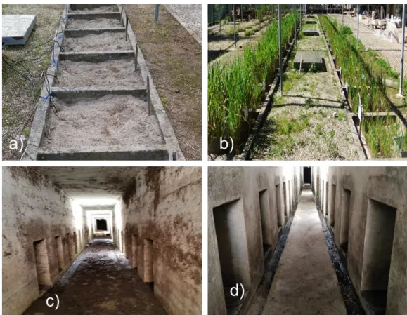
Koon et al., 2009). ... 9 Figure 2.3 – Calculation sequence utilized by RZWQM2 (adapted from Ahuja et al., 2000a). ...15 Figure 2.4 – Diagram of residue and soil organic matter pools in RZWQM2 (Adapted from Cameira et al., 2007). ...18 Figure 3.1 – Drainage lysimeters existing at Horto facilities (Adapted from Martins, 2014). (Letters designate the slurry treatments as described in 3.1.2) ...22 Figure 3.2 – Lysimeters: a) top view with bare soil; b) top view with oats crop; c) access tunnel beneath the lysimeters before recuperation; d) access tunnel cleaned and in use. ...23 Figure 3.3 - Monthly mean maximum and minimum temperatures and monthly precipitation during the study period, with the 30 years’ average (1951-1980), collected from the meteorological station of Tapada da Ajuda. ...24 Figure 3.4 - Representation of the lysimeters used for this work, with the slurry treatments and both soils. (Adapted from Martins, 2014) ...25 Figure 3.5 - a) Reflectometers installed in lysimeters for the measurement of SWC; b) Lysimeter with both chambers for the measurement of NH3 volatilization (round) and N2O
(square). ...29 Figure 3.6 – General view of the installed equipment. ...29 Figure 3.7 – Simple modelling procedure overview (adapted from Ma et al., 2012). ...30 Figure 3.8 - Graphical representation of the simulation domain and boundary conditions. ....31 Figure 4.1 - Hydraulic properties of the sandy soil described by the Brooks and Corey functions before (BC) and after (AC) calibration: a) Water retention; b) Saturated hydraulic conductivity. ...40 Figure 4.2 - Simulated versus measured values for: a) soil water content at 25 cm and b) drainage at 100 cm. Sandy soil, 2014-2015 crop season (calibration). (FC10 is the soil water
iii
Sandy soil, 2014-2015 crop season (calibration). ...42 Figure 4.4 - Simulated versus measured values of: a) NO3- flux at the depth of 70 cm; b) N2O
emissions at soil surface. c) Water filled pore space. Sandy soil, 2014-2015 crop season (calibration). ...43 Figure 4.5 - Simulated versus measured values correlation comparison for: a) soil water content; b) drainage; c) nitrate leaching and d) N2O flux to the atmosphere. Sandy soil,
2014-2015 (calibration). ...45 Figure 4.6 - Hydraulic properties of the sandy loam soil described by the Brooks and Corey functions before (BC) and after (AC) calibration: a) Water retention; b) Saturated hydraulic conductivity. ...47 Figure 4.7 - Simulated versus measured values for: a) soil water content at 20 cm and b) drainage at 100 cm. Sandy loam soil, 2014-2015 crop season (calibration). (FC10 is the soil water content at field capacity at 10 kPa.) ...48 Figure 4.8 - Simulated versus measured values for the soil temperature at the depth of 25 cm. Sandy loam soil, 2014-2015 crop season (calibration). ...48 Figure 4.9 - Simulated versus measured values of: a) NO3- flux at the depth of 70 cm; b) N2O
emissions at soil surface. c) Water filled pore space. Sandy loam soil, 2014-2015 crop season (calibration). ...50 Figure 4.10 - Simulated versus measured values correlation comparison for: a) soil water content; b) drainage; c) nitrate leaching and d) N2O flux to the atmosphere. Sandy loam soil, 2014-2015 (calibration). ...52 Figure 4.11 - Simulated versus measured values for: a) soil water content at 25 cm and b) drainage at 100 cm. Sandy soil, 2015-2016 crop season (validation). (FC10 is the soil water content at field capacity at 10 kPa.) ...53 Figure 4.12 - Simulated versus measured values for the soil temperature at the depth of 25 cm. Sandy soil, 2015-2016 crop season (validation). ...54 Figure 4.13 - Simulated versus measured values of: a) NO3- flux at the depth of 70 cm; b) N2O
emissions at soil surface. c) Water filled pore space. Sandy loam soil, 2012-2013 and 2013-2014 crop seasons (validation). ...55 Figure 4.14 - Simulated versus measured values for: a) soil water content at 20 cm and b) drainage at 100 cm. Sandy loam soil, 2015-2016 crop season (validation). (FC10 is the soil water content at field capacity at 10 kPa). ...56 Figure 4.15 - Simulated versus measured values for the soil temperature at the depth of 20 cm. Sandy loam soil, 2015-2016 crop season (validation). ...57
iv
emissions at soil surface. c) Water filled pore space. Sandy loam soil, 2012-2013 and 2013-2014 crop seasons (validation). ...57 Figure 4.17 - N output from crop-soil system comparison for sandy soil (top) and sandy loam soil (bottom), in the different precipitation scenarios: a) very dry; b) dry; c) medium and d) wet. ...62 Figure 4.18 – N2O and NH3 variation for all hydrological years, in comparison with Vdy in the
a) sandy soil and b) sandy loam soil (VDy – very dry; Dy – dry; M – medium; W – wet; N2O – N2O emission losses; NH3 – NH3 volatilization losses). ...62
Figure 4.19 – Contribution of nitrification and denitrification for the total N2O emission for: a)
sandy soil and b) sandy loam soil. (VDy – very dry; Dy – dry; M – medium; W – wet; N2O Nit - N2O resulting from nitrification process and N2O Denit - N2O resulting from denitrification
process). ...63 Figure 4.20 – Variation in Ngas losses during the temperature scenarios. Sandy and sandy loam
soils. ...63 Figure 4.21 – Variation of NH3 volatilization during the temperature scenarios, in comparison
with M scenario. Sandy and sandy loam soils. ...64 Figure 4.22 – Contribution of nitrification and denitrification for the total N2O emission for: a)
sandy soil and b) sandy loam soil. (N2O Nit - N2O resulting from nitrification and N2O Denit -
N2O resulting from denitrification). ...65
Figure 4.23 - N output from crop-soil system comparison for sandy soil (top) and sandy loam soil (bottom), in the different temperature scenarios: a) M; b) B1 and c) A1F1. ...65 Figure 4.24 – Drainage fluxes at 70 cm depth, average for all slurry treatment in the SS. ....66 Figure 4.25 - Nitrate flux means comparison between slurry treatments of the sandy soil, for the (a) 2012-2013, (b) 2013-2014 and (c) 2014-2015 crop seasons. ...69 Figure 4.26 - Drainage fluxes at 70 cm depth, average for all slurry treatment in the SLS. ...70 Figure 4.27 - Nitrate flux means comparison between slurry treatments of the SLS, for the (a) 2012-2013, (b) 2013-2014 and (c) 2014-2015 crop seasons. ...71
v
Table 3.1 - Main soil physical properties ...23
Table 3.2 - Measurement dates and equipment utilized for relevant variables ...26
Table 3.3 – Temporal domain for each crop season and correspondent modelling phase ....31
Table 3.4 – Model input data and respective sources ...32
Table 3.5 - Parameterization of the basic soil physical properties ...32
Table 3.6 - Parameterization of the Brooks and Corey hydraulic functions ...33
Table 3.7 - Nitrogen nutrient efficiency factors and reaction rates parameterization ...33
Table 3.8 - Plant and crop parameterization ...34
Table 3.9 - Crop management events for each crop season, in both sandy and sandy loam soils ...34
Table 3.10 - Dairy cattle slurry characterization ...34
Table 3.11 - Thermal properties of soil constituents (after de Vries, 1963) ...35
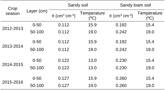
Table 3.12 - Soil water content and temperature initial conditions for each crop season ...35
Table 3.13 - Selected parameters for calibration and respective control data ...36
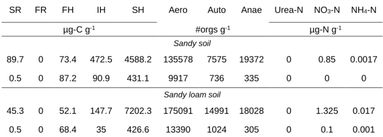
Table 3.14 - Initial residue state, microorganism and inorganic N profile after wizard and 10 year equilibration, for both soils ...37
Table 4.1 - Initial and calibrated values of the selected soil hydraulic parameters. Sandy soil ...40
Table 4.2- Initial and calibrated values for the OM partitioning and for N related parameters. Sandy soil, 2014-2015 crop season (calibration) ...43
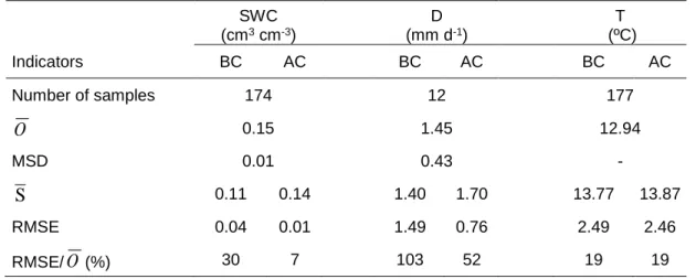
Table 4.3 - Goodness of fit analysis for the soil water content at 25 cm, water drainage at 100 cm depth and soil temperature at 25 cm depth, before (BC) and after (AC) model calibration. Sandy soil (2014-2015) ...44
Table 4.4 - Goodness of fit analysis for NO3- and N2O emissions after model calibration. Sandy soil (2014-2015). ...46
Table 4.5 - Initial and calibrated values of the selected soil hydraulic parameters, for the sandy soil loam soil ...46
Table 4.6 - Initial and calibrated values for the OM partitioning and for N related parameters. Sandy loam soil, 2014-2015 crop season (calibration) ...49
Table 4.7 - Goodness of fit analysis for the soil water content at 25 cm, water drainage at 100 cm depth and soil temperature at 25 cm depth, before (BC) and after (AC) model calibration. Sandy loam soil (2014-2015) ...51
Table 4.8 - Goodness of fit analysis for NO3- and N2O emissions after calibration. Sandy loam soil (2014-2015). ...52
vi
and T at 25 cm (2015-2016) and the NO3 flux and N2O emission flux (2012-2013 and
2013-2014). Sandy soil. ...55 Table 4.10 - Goodness of fit analysis for the validation of soil water content, water drainage at 100 cm depth and temperature (2015-2016 crop season) and the NO3- flux and N2O emission
flux (2012-2013 and 2013-2014 crop seasons). Sandy loam soil ...58 Table 4.11 – Soil water balance for the precipitation scenarios. Sandy and sandy loam soils (04/11 to 22/04), ...60 Table 4.12 – Nitrogen balance for precipitation scenarios. Sandy and sandy loam soils, 2013-2014 crop season ...61
vii
A1F1 IPCC climate change scenario, increase of 4ºC in average temperature
ANOVA Analysis of variance
AOB Ammoniaoxidising bacteria
AWSM Acidified whole slurry mobilization application
AWSS Acidified whole slurry surface application
B1 IPCC climate change scenario, increase of 1.8ºC in average temperature
CAP Common Agricultural Policy
CTR Control
Dy Dry
EU European Union
FAO Food and Agriculture Organization
IPCC Intergovernmental Panel on Climate Change
IPPC Integrated Pollution Prevention and Control
KW Kruskal-Wallis
M Medium
ND Nitrates Directive
NEC National Emission Ceilings
OMNI Organic Matter/Nitrogen model
ppb Parts per billion
RZWQM2 Root Zone Water Quality Model
SLS Sandy loam soil
SS Sandy soil
UK United Kingdom
USDA United States Department of Agriculture
UWWD Urban Waste Water Treatment Directive
VDy Very dry
W Wet
WFD Water Framework Directive
WSI Whole slurry injection application
viii
Symbol Physical variable
C/N Carbon to nitrogen relation
CEC Cation exchange capacity
CO2 Carbon dioxide
K(h) Hydraulic conductivity function
LAI Leaf area index
LPW Litres of pore water
N Nitrogen N2 Dinitrogen gas N2O Nitrous oxide NH3 Ammonia NH4+ Ammonium N-NH4+ Ammonium as nitrogen
N-NO3- Nitrate as nitrogen
NO Nitric oxide
NO3- Nitrate
pH Power of Hydrogen
ix
Physical
variables Physical name SI Units
A2 Pore size distribution index dim
Aero Aerobic heterotrophs org g-1
AET Actual evapotranspiration mm
Anae Anaerobic heterotrophs org g-1
aNH4 Autotroph converting nitrified NH to autotroph biomass-N frac
Auto Autotrophs org g-1
BD Bulk density g cm-3
BM Biomass converting organic matter uptake frac
C0, C1 Reflectometers calibration coefficients dim
C1 Saturated hydraulic conductivity cm h-1
C2 Second intercept on conductivity curve dim
Cv Volumetric heat capacity J mm-3 ºC-1
D Soil water drainage mm d-1
DENIT Denitrification constant d-1
DENITOM Denitrification rate converting to anaerobic organic matter
decay rate dim
EC Electrical conductivity µS cm-1
EF Modelling efficiency %
FH Fast soil humus µg C g-1
FR Fast residue µg C g-1
h Soil water matrix pressure cm
IH Intermediate soil humus µg C g-1
Kc Thermal conductivity J mm
-3 h-1
ºC-1
kNH3 NH3 volatilization constant km d-1
Ks Saturated hydraulic conductivity cm h-1
MSD Mean standard deviation of observations *
n Total number of observations #
N2 Second exponent for conductivity curve dim
N2N2O Denitrification efficiency factor frac
Nfert Total N input from fertilization kg ha-1
Nfert N input from fertilization kg ha-1
Ngas N lost in the gaseous form kg ha-1
NIT Nitrification constant mol LPW
-1
d-1
NITN2O N2O fraction from nitrification constant frac
Nleach N lost from drainage kg ha-1
Nuptk N uptake by the plant kg ha-1
Õ Measured mean *
Ok kth observed value *
OM% Organic matter percentage in slurry %
x
Pk kth simulated value *
R2 Coefficient of determination frac
RMSE Root mean square error of simulations *
S1 Bubbling pressure cm
S2 Bubbling pressure cm
SDk Standard deviation for kth level *
SfN Final stored mineral N in the soil kg ha-1
SH Slow soil humus µg C g-1
SiN Initial stored mineral N in the soil kg ha-1
SN-NH4+ Amount of ammonium in the slurry kg ha-1
SR Slow residue µg C g-1
SWC Soil water content in the soil cm3 cm-3
T Soil temperature ºC
Tmax Monthly mean maximum temperature ºC
Tmin Monthly mean minimum temperature ºC
VHC Dry volume heat capacity J mm-3 C-1
WFPS Water filled pore space %
yk kth measured value *
ŷk kth predicted value *
ӯ Measured mean *
ΔSN Variation of the mineral N stored in the soil, kg ha-1
Porosity cm3 cm-3
N2O Nitrous oxide emissions flux kg ha-1
NO3- Nitrate leaching flux kg ha-1
Soil water content in the soil cm3 cm-3
10 Soil water content at 10 kPa (Field capacity) cm3 cm-3
15 Soil water content at 33 kPa (Field capacity) cm3 cm-3
33 Soil water content at 1500 kPa (Wilting point) cm3 cm-3
r Residual water content cm3 cm-3
s Water content at saturation cm3 cm-3
1
1. Introduction
During the 20th and 21st centuries, a large increase in food and animal feed production occurred,
as a response to the increasing human population in the world, and consequent food demand. This lead to the intensification of agriculture in many regions of the globe, with the increased use of resources namely water and fertilizers over the past 50 years (Smil, 2000; 2001). In some world regions, including Europe, the agriculture intensification led to numerous environmental problems, directly or indirectly affecting human health, such as greenhouse gases emission, water bodies’ contamination with nitrates and other ecosystem vulnerabilities. (Mosier et al., 2004; Tedesco, 2013). Agriculture is actually seen as one of the main N pollution sources through the diffuse emission of ammonia (NH3) and nitrous oxide (N2O) to air and
nitrate (NO3-) to surface and ground waters (Oenema et al., 2011).
The legislation, technologies and measures to reduce N emissions exist, but the diversity of the cropping systems and the complex diffuse N pathways have resulted in regulatory obligations, which are not equally efficient for different type of production system (Cameira & Mota, 2016). Also, as recent studies have highlighted (Stevens & Quinton, 2009; Agostini et
al., 2010) there is the danger of pollution swapping between NO3- leaching and N2O and NH3
gaseous losses, which requires a holistic approach to the diffuse pollution issue, including the N dynamics and management in the soil-plant-atmosphere systems.
One important tool for the application of this integrated or holistic approach is the use of system modelling, where the interactions between the different components of an agricultural system are considered. Thus, the different N transport and transformation processes occurring at the different compartments are accounted for and related with the water regime of the soil. This constitutes the modelling approach used in the present work, through the evaluation and application of the RZWQM2 model.
The present study, which was developed under the scope of scientific Project PTDC/AGRPRO/119428/2010, had the general objective of modelling the N emissions from a winter oat crop fertilized with dairy cattle slurry. More particularly it was intended to:
- Calibrate and validate the RZWQM2 model for a sandy soil and a sandy loam soil under a whole slurry application followed by incorporation;
- Make a comparative analysis between both soils with respect to both path losses for NO3
-leaching and N2O emissions to the atmosphere;
- Conceptually relate the different types of losses with the soil water regimes and temperatures;
2
- Analyse different scenarios to predict the N losses under different hydrological years and a climatic change perspective using a 30 years’ data series;
- Estimate the nitrate fluxes (φNO3-) under different slurry treatments using the predicted soil
water and drainage and the measured nitrate concentration in the soil solution. Perform an analysis of variance to find differences between treatments’ effect in the NO3- leaching flux.
The current work is divided in 5 chapters. In chapter 2, the literature review, the relevance of the study is justified and the theoretical bases needed to understand the results are presented. Chapter 3 describes the materials and methods used for data collection and treatment and the methodology for the modelling procedure. Chapter 4 presents the results obtained for model calibration and validation as well as the ones relative to scenario analysis under a climatic change perspective. The results of the variance analysis applied to the nitrate leaching for the different slurry treatments are also presented. Finally, Chapter 5 summarizes the main conclusions of the present work and presents some consideration about the future perspectives for further studying this subject.
The collection of climate related variables was done, in the Meteorological Station of Tapada da Ajuda, and the sampling of NO3- concentration in the soil solution and N2O emissions during
the autumn/winter seasons from 2012 to 2014) were not performed by the author of the present work, as they were done by colleagues. The soil water content (SWC) and soil temperature (T) measurements as well as the water drainage (D) collection under the lysimeters were performed by the author during the autumn/winter season of 2015-2016, as well as all of the modelling work.
3
2. Literature review
This chapter presents the theoretical aspects necessary for the understanding the type of problem studied in this work and the information necessary to interpret the results.
2.1 Diffuse pollution and nitrogen emissions
Diffuse or non-point source pollution refers to both water and air pollution caused by a variety of activities that have no specific point of discharge. In addition, the long-range transport ability and multiple sources of the pollutant contribute to the diffuse nature of the process. The management of diffuse pollution is complex and requires the careful analysis and understanding of various processes (WMO, 2013).
Agriculture is one of the main N diffuse pollution sources. N loss through gaseous emissions, primarily in dinitrogen gas (N2), N2O and NH3, is one of the most significant loss of N from the
crop-soil system (Chen et al., 2014). N2O not only contributes to climate change, it has a large
radioactive-forcing potential with long-term warming potential 298 times greater than carbon dioxide (CO2), but it also induces the depletion of the ozone layer (Cameron et al., 2013).
Approximately 62% of total global N2O emissions are attributed to agricultural soils and
non-agricultural land (Thomson et al., 2012).
There are several sources of N2O emissions from agricultural soils, e.g. the application of
synthetic fertilizers, manure/slurry and other organic fertilizers, biological fixation by the crops and the mineralization of crop residues. Following a methodology revision (Moisier et al., 1998), by request of OECD/IPCC/IEA three types of emissions are considered: (i) direct emissions; (ii) emissions from animal production; and (iii) indirect emissions (Mosier et al., 1998). However, only direct and indirect emissions of N2O are within scope of the present study.
Direct emissions include those where N2O is emitted directly into the atmosphere from the soils,
with agriculture appearing as a major contributor, mostly through biogenic production of N2O,
i.e. nitrification and denitrification processes (IPCC, 1995a; Bouwman et al., 1995; Parton et
al., 1996).
Indirect emissions are due to: (a) the transport process that N suffer, from the soil-plant system into ground and surface waters through deep drainage and surface runoff; or (b) emissions as NH3 or nitrogen oxides (NOx) posteriorly suffering deposition elsewhere, inducing N2O
4
2.2 Nitrogen pathways and processes
To choose the mitigation practice more suitable for each production system it is necessary first to identify the main path for the N losses (e.g. leaching or gas loss) for that system as well as the most important N transformations (e.g. nitrification, denitrification, volatilization).
2.2.1 The importance of soil water
2.2.1.1 Soil water and the N losses
Most of the cases of N loss from farming practices are caused by its transport with excess of water over and/or through the agricultural soil (Carpenter, 2008). This physical process is called convective transport or N leaching). On the other hand, the soil moisture will influence the biological and chemical reactions that determine the N form present in the soil and consequently the N available for the plant (see section 2.2.2).
As such, controlling the water flow from the agricultural field to the surface and ground waters is one of the most important practices to reduce N loss and pollution. The influence of soil moisture in the N related processes and transport is within the scope of the present study and shall be further discussed below.
The soil physical properties (such as bulk density, porosity, soil texture), the soil hydraulic properties consisting in the soil water retention curve and the soil hydraulic conductivity curve, and the basic chemical properties (e.g. pH, and organic matter (OM) content) are important to understand a given N-related process. In fact, both the water transport flux and soil water content (SWC) depend heavily in the soil hydraulic/hydrodynamic and, to some extent in the chemical properties. Only knowing these soil properties that it is possible to assess/evaluate and predict the N impact in the environment, devising a suitable mitigation measure.
2.2.1.2 Soil water balance
In order to determine the amount of water (W) in the soil at any given moment of time and to minimize the excess of drainage, the following water balance equation is used:
Ro
D
AET
P
Irr
ΔS
W
[2.1]where S is the variation of stored water in the soil (initial-final), P is the precipitation, Irr is irrigation, AET is the actual evapotranspiration, D is the drainage, Ro is runoff. All terms are in mm. Both P and Irr are water input terms, while D, AET and RO are water outputs/ from the soil. D it is the most important N loss pathway (N leaching) especially for the rainy seasons as it is not possible to control precipitation. For the spring/summer seasons, if irrigation is well designed and managed, N leaching can be minimized. D occurs when the stored water in the
5
soil is higher than the field capacity, yielding higher values for coarser soils and lower for finer texture soils.
2.2.2 Forms and transformations of N in the soil
N is subject to process of many natures in the crop-soil system, related to storage, transformations and transport. As a result, N can be found in many forms in the soil, being the four major forms: (i) organic matter (OM), as plant material, fungi and humus; (ii) soil organisms and microorganisms; (iii) ammonium ions (NH4+) adsorbed to clay minerals and OM and; (iv)
mineral N forms in the soil solution, including NH4+, NO3- and nitrite (NO2-) in low concentrations.
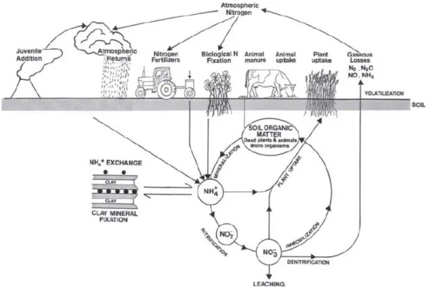
All the transformations and forms of N in an agricultural system are illustrated in Figure 2.1. The preferred forms of nitrogen for plant absorption are NH4+ and NO3- (Cameron et al., 2013).
While the atmosphere is the largest reservoir of N (Schlesinger, 1991), most of this N is in the molecular form (N2), which is not directly available to most plants. Over 90% of the N in most
soils is in organic form (Stevenson, 1982).
Figure 2.1 – Nitrogen cycle in the crop-soil system (adapted from Cameron, 1992). 2.2.2.1 Nitrogen fixation
Fixation is the conversion of molecular N, present in the atmosphere, into biologically available forms (Boyer et al., 2002), that may be incorporated in organic materials by specific microorganisms (Nicolardot et al., 1997). Biologically, this conversion is conducted by aerobic or anaerobic microorganisms. The most relevant factors affecting this process are:
6
Soil moisture: The microorganism primarily responsible for this process (cyanobacteria) are only physiologically active when wet (Nash, 1996). Soil water is necessary for C fixation by the cyanobacteria, because N fixation depends upon products of photosynthesis, which by turn requires water (Belnap, 2001).
Soil temperature: N fixation is also controlled by soil temperature, with most soil cyanobacteria being capable of N fixation between -5 and 30 ºC, whereas optimum temperature for this activity ranges from 20 to 30 ºC. Out of this range the N fixation rate rapidly declines (Belnap, 2001).
pH: Microorganism growth and N fixation in soil is increased at pH 7 or above (Dubois & Kapustka, 1983). However, some decline in the microbial activity has been found at pH 8-10 (Granhall, 1973).
Other: High concentration of aluminium (Al) and/or manganese (Mn) in the soil inhibit the activity of N fixing bacteria (Carranca, 2000).
2.2.2.2 N mineralization
According to Crohn (2004), mineralization consists in the conversion or degradation of the organic N into mineral N forms, performed by the microorganisms that need of the organic N as energy source. It is a two-step process, with the initial step known as aminization, which consists of the decomposition of complex proteins/nitrogenous contained in the organic substances, present in the soil, into simpler material like amino acids, amines and amides, alongside CO2 and energy:
Energy
matter
Organic
RNH
2
CO
2
[2.2]where RNH2 are the amines and amino acids, and CO2 is carbon dioxide
The resulting amino groups may be used by the microorganisms in the soil to form their own structure or further converted in simpler compounds of NH3, which is the end-product alongside
energy and sometimes CO2, of the second-phase of this process, ammonification:
Energy
ROH
O
H
RNH
2
2
[2.3]where ROH is an alcohol functional group.
Based on Scheppers & Mosier (1991) rule of thumb to estimate the annual N mineralization is to consider that it should be around 20 kg ha-1 year-1 per each 1% of soil endogenous OM, for
the top 30 cm. Mineralization depends of environmental factors affecting microbial growth and activity:
7
Moisture: Based on Killham et al., (1993), water availability in the soil not only seems to have a positive effect on microbial growth and nutrition, but it also increases the ability of a microorganism to reach the substrate, consequently increasing N mineralization rate. Meanwhile low soil moisture induces negative effects in the N mineralization rate, due to increasing osmotic pressure, which in turn increases the energy required for osmoregulation of the microorganisms (Harris, 1981). The optimum range of moisture for mineralization is between field capacity and 40% of field capacity (Campbell & Biederbeck 1982).
Temperature: Increases in this state variable have a positive effect in the N mineralization rate (Zak et al., 1999), being the optimum range of temperature between 25 and 35 ºC (Honeycutt and Metcalf, 1994).
pH: The optimal pH for soil biomass growth has been established near neutrality, with mineralization being restricted at low pH levels (Appel & Mengel, 1990).
Salinity: A high salt content in the soil solution has been reported as having a negative effect in biomass growth, and consequently in N mineralization (Laura, 1977), which is related to the required osmoregulation of the microbial tissues in these conditions.
C/N relation: According to Tisdale et al. (1985), the C/N relation of any substance applied to the soil will affect the mineralization rate. If C/N is between 20:1 and 30:1, the mineral N will be released at an equilibrated rate, in relation to plant uptake rate. Above 30:1, more immobilization is verified during the initial stages of the decomposition process due to the lack of mineral N in the substance; Below 20:1 the release rate of mineral N from the substance is too fast and the loss potential increases (Bengtsson, 2003).
2.2.2.3 Fertilization
Different forms of N can be added into the soil, directly and indirectly, through fertilization and/or soil melioration applications. In the case of fertilization, where the applied substance supplies relevant nutrients directly to the plant, the majority of N-based fertilisers derive from NH3, which is synthetized with the widely used industrial N fixation process of Haber-Bosch,
where N2 is fixed chemically, at high temperature and pressure, producing NH3. Whereas the
soil improvers, that indirectly help the plant growth by enhancing the soil quality, which indirectly helps the plant growth, are generally organic materials, such as animal manures and green composts.
2.2.2.4 Plant uptake
The preferred N forms for plant uptake are NH4+ and NO3-, while NO2- and other simple organic
8
plants absorb NO3- predominantly, as in well aerated and neutral pH soils, this is the N form
present in highest concentrations (Tisdale et al., 1985). 2.2.2.5 N volatilization
This process, involving physical, chemical and biological factors, consist in the loss of N from the soil-crop system through the surface layer in the form of NH3, which results from the
accumulation of N-NH4+ in soils with high soil moisture.
O
H
NH
OH
NH
4
3
2 [2.4]This process is influenced by the following factors:
Temperature: NH3 volatilization increases with temperature, as observed by Ball & Keeney
(1979), with the optimum range being from 25-30 ºC (Sommer et al., 1991). Nonetheless, a few studies have shown that the amount of N lost via volatilization may not be different at low versus high temperature, since volatilization may continue for longer at low temperatures (e.g. Harper et al., 1987). Nonetheless, the initial volatilization is slow for temperatures below 15ºC (Sommer et al., 1991).
pH: Higher pH tend to lose more NH3 gas (Sommer et al. 2004), though neutral or acid pH
soils may also loose significant amounts when urea or animal urine are applied (Black et al., 1985a,b), i.e. higher pH promote NH3 volatilization.
NH4+ concentration: Generally, a high concentration of NH
4+ in the soil solution induces a high
potential emission rate of NH3 gas. Therefore, the application of N fertilizers in this form and
animal dejects (slurry and/or urine) can significantly enhance the NH3 emission rate. The NH4+
concentration in the soil depends of several factors like nitrification rate, plant uptake rate, denitrification rate and immobilization rate, all of which reduce the NH4+ concentration
(Cameron et al., 2013).
Moisture: Soil moisture influences the concentration of NH3/ NH4+ in the soil solution, with low
values inducing higher concentrations and thus promoting higher NH3 volatilization (Cameron et al., 2013). Nonetheless, Al-Kanani et al. (1991) found that at very low SWC, the rate of NH3
emission will be slow. In situations where there is a significant input of water through rainfall or irrigation the NH3 volatilization can be reduced, because the water transports the N far from
the soil surface where the concentration of NH4+ is kept low (Black et al., 1987).
Other: The mechanism of soil cation exchange (CEC) helps in storing NH4+ in the soil thus,
concentration in the soil solution. Additionally, CEC helps to buffer against pH changes, i.e. it high CEC implies lower NH3 volatilization potential and low CEC implies higher potential
9
The potential risk of ammonia volatilization from urea fertiliser can represent between 0% and 65% of the N applied, depending on soil and climatic conditions (Bishop & Manning, 2010). Whereas, the greatest risk of NH3 volatilization occur with the use of ammonium bicarbonate,
urea and ammonium hydroxide based fertilizers (Whitehead & Rastrick, 1990). Volatilization losses from poultry manure and dairy slurry was found to be 9-20 % and 14-35% of total N applied respectively (Miola et al. 2014; Sadeghpour et al. 2015).
2.2.2.6 Nitrification
According to Mosier et al. (1998) nitrification consists of the aerobic microbial oxidation of NH4+
into NO3-, via NH2OH (hydroxylamine), as shown below:
3 2 2 4NH
OH
NO
NO
NH
[2.5]This process may be divided in 2 phases, conducted by the activity of two different autotrophic bacteria. Firstly, the oxidation of NH4+ to NO2- is due to soil ammonia-oxidising bacteria (AOB),
such as Nitrosospira and Nitrosomonas (Prosser, 2007). The second phase, the oxidation of NO2- to NO3- is conducted by Nitrobacter, characterized as occurring very rapidly which makes
NO2- accumulation in the soil somewhat rare. The nitrification process described above is
detailed in Figure 2.2, showing that the oxidation of NH4+ can also produce N2O (Cameron et al., 2013):
Figure 2.2 – Nitrification and denitrification, with both N2O formation pathways (adapted from Koon et al., 2009).
The production of N2O from NH4+ and NH2OH, an intermediary compound, is possible thanks
to the activity of AOB, such as Nitrosospira and Nitrosomonas (Zaman et al., 2009). The main factors that affect the nitrification process in the soil are:
10
Temperature: Nitrification intensifies as temperature increases, with the optimum soil temperature for nitrifying bacteria being between 25 and 30ºC (Haynes et al., 1986). Nonetheless, nitrification still occurs at temperatures below 5ºC, but the rates is significantly slower than at higher temperatures (Cameron et al., 2013).
pH: The bacteria responsible for this process normally operate at pH ranges from 5.5-8, with the optimum soil pH range being from 4.5 to 7.5 (Haynes et al., 1986).
Moisture and aeration: As the soil gets wetter, i.e. more prone to anaerobic conditions, nitrification rate decreases, as these microorganisms are typically aerobic. Nitrification rate is also significantly slower when the soil is dry, although it still can occur at wilting point (-1500 kPa) (Monaghan & Barraclough, 1992).
The maximum nitrification rate occurs around soil moisture content at field capacity (-10 kPa) (Haynes et al., 1986).
Ammonium concentration: As shown in the reaction equation [2.5], the whole process of nitrification is dependent of the NH4+ available in the soil, however high concentration of NH4+/
NH3 can restrict the activity of Nictrobacter (Monaghan & Barraclough, 1992).
2.2.2.7 Denitrification
Denitrification is a reductive process, which mainly occurs in poorly drained soils where there are anaerobic soil conditions, low oxygen availability and low redox conditions (Dobbie & Smith, 2001; Bateman & Baggs, 2005). This permits facultative anaerobic bacteria to use NO3-,
instead of O2, as the final electron acceptor during respiration with NO3- being reduced,
producing NO2-, nitric oxide (NO), N2O and finally N2, which can escape from microbial cells to
the soil atmosphere (Cameron et al., 2013), reaction that is shown below:
N O N NO NO NO3 2 2 2 [2.6]
The main factors that affect denitrification are:
Temperature: Ryden (1986) and Dobbie & Smith (2001) show that the denitrification rate increases with temperature. For example, the denitrification rate increased by 10-times in a grassland when the temperature increased from 10ºC to 20ºC (de Klein & van Logtestijn, 1996). pH: Haynes & Sherlock (1986) states that acid soils with pH lower than 5.0 have lower denitrification rates than agricultural soils with a typical pH around 6.0, taking into account that the N2O/N2+N2O ratio increases with acidity (Thomson et al., 2012).
Moisture and aeration: The soil moisture content has a big influence in the denitrification rate. When soil moisture content is greater than field capacity, a significant increase in the potential denitrification is verified (Moisier et al., 1986). A high soil moisture is associated with anaerobic
11
conditions, meaning that there is a larger water filled pore space (WFPS), with denitrification greatly increasing as WFPS increases (Rabot et al., 2015). More specifically, once WFPS exceeds 0.6 (60%) of the soil pore space, denitrification starts to intensify rapidly (Dobbie et
al. 1999).
Nitrate and ammonium availability: The availability of N (NH4+ and NO3-) in the soil has a big
influence upon the denitrification rate, with emissions generally increasing due to increases in mineral N in the soil (Saggar et al., 2009). It is worth noting that the anthropologic input of N, through N fertilizer and animal excreta application, often increases the availability of mineral-N in the soil, which can induce very large denitrification rates in the appropriate conditions (de Klein et al., 2001).
Carbon in the soil: Increases in the amount of readily available organic C, from the application of organic waste or animal manure, stimulates the denitrification process (Di & Cameron, 2003), since it is widely established that there is a strong relationship between readily available organic C in the soil and the denitrification rate (Burford & Bremner, 1975).
2.2.2.8 N Leaching
Leaching is the process through which N is lost from the soil root zone to ground and surface waters. It can be described by a combination of three physical processes: convection, diffusion and hydrodynamic dispersion (Hillel, 1998). The convective transport occurs due to the mass flow of water through the soil during drainage events after precipitation and/or irrigation (Cameira & Mota, 2016). It is calculated by modified form of Darcy’s law.
dx dH K C C D NO3 NO3 NO3
[2.7]where
NO3-is the convective NO3- flux, CNO3 is the N-NO3- concentration, D is the water fluxor drainage, K is the hydraulic conductivity and dH/dx is the hydraulic gradient.
This implies uniform displacement of the band of NO3-, which in reality, the band of NO3- tends
to spread throughout the profile because of the processes of diffusion and hydrodynamic dispersion. The diffusive transport results from a concentration gradient between the band of NO3- and the surrounding soil, there is a diffusive flux of NO3- from the band of NO3- into the
surrounding soil, described by Fick’s law.
dx dc DS
Jd [2.8]
where Jd is the rate of diffusion, DS is the diffusion coefficient of the NO3- in the soil which
12
Hydrodynamic dispersion is due to (a) non-uniformity of the flow velocity within a single pore; (b) large variations in pore size in the soil, which causes a range of pore water velocities and (c) the ‘tortuosity’ of soil pores produces a range of flow path lengths. Thus, combining the three mechanisms, NO3-, is given by the convection-dispersion equation, which is used by
the process based mathematical models that simulate the leaching process:
x
c
U
x2
c
2
Da
t
c
[2.9]where Da is the apparent diffusion coefficient which represents the sum of molecular diffusion
and hydrodynamic dispersion.
The form of N most susceptible to leaching is the NO3-, since as it is negatively charge it will
not be retained in the CEC. On the other hand it is very soluble in water and is the mineral form found in higher concentrations in the soil (Countinho-Mendes, 1989). The NO3- in the soil
is produced by the nitrification process. The amount of leached NO3- depends on one hand
upon the concentration of NO3- in the soil (which in turn, strongly depends on the amount of
applied N, the nitrification and denitrification rates), and on the other hand it depends upon the amount of drainage that occurs through the soil which will carry the NO3- (convective transport).
Nonetheless, there are other soil factors that also affect NO3- leaching and are far more difficult
to describe mathematically because of their transient nature and complexity:
Climate: N losses through NO3- leaching are usually higher in late-autumn, winter and
early-spring months, when plant uptake of N is low because of cooler conditions and drainage is high due to rainfall inputs exceeding evapotranspiration demands (Wild & Cameron, 1980). Whereas a dry summer may result in an accumulation of NO3- in the soil since no drainage
occurred, this NO3- can be leached over the upcoming winter. Furthermore, the rewetting of
the soil after a dry summer can cause a big and sudden increase in mineralization and thus originating more N leaching (Scholefield et al., 1993).
Soil properties: Soil texture and structure affects N losses through leaching, as it influences the water movement in the soil. NO3- leaching is generally greater in more poorly structured
sandy soils than from clay soils, alongside a greater denitrification potential in clay soils. Macrospores created by the living beings in the soil or the wetting and drying cycles, induce a quicker leaching of NO3- through the soil profile (Cameron et al., 2013).
Others: Irrigation during summer does not generally cause leaching, unless excessive amounts of water are applied causing drainage events. This is because irrigation increases plant growth, and consequently plant N uptake, reducing the potential for NO3- leaching losses
13
and frequency/rate of application have a large influence in the NO3- leaching, after fertilization
application. The same factors are verified in the organic manures and waste application, with the addition of manure type. The efficiency of fertilization is an important factor to consider when dealing with NO3- leaching, as it will dictate the amount of available N that is not
recovered by crops, to be lost through leaching, and other process. Jenkinson (2001) found that when N fertiliser is applied at rates that match cereal plant demand, there is no residual mineral fertiliser-N left in the soil at harvest.
2.2.2.9 N budget in the soil
In order to determine the amount of mineral-N in the soil at any time, Wild & Cameron (1980) and Di & Cameron (2002a) recommend the following N balance equation based on the N cycle:
Ne Ni Nleach Ngas Nuptk Nmin Nfert Nb Np N [2.10]
where p is the N provided by precipitation and dry deposition, b is biological fixation, fert is fertilizer more urine and dung/slurry, min is mineralization, uptk is plant uptake, gas is gaseous losses, I is immobilization, leach is leaching loss and e is erosion and surface runoff.
2.3 Environmental and health impacts related to nitrogen
Inputs of N in the soil causes a “cascading” effect and a broad range of changes, which have effect/impacts on humans and ecosystems in many ways all over the world (Galloway & Cowling, 2002). Adapting the “cascade model” in Appendix 1, it illustrates the multiple effects N has in the environment, alongside the complexity in reducing one emission pathway without considering the total N supply (Erisman et al., 2005).
The most common impacts associated to agriculture are related with the contamination of surface and ground waters with NO3-, and atmospheric air with NH3 and greenhouse gases.
These losses of N in the soil have a negative impact on the environment, and consequently on humans. The potential negative impacts are: drinking water contamination, acidification and eutrophication of natural ecosystems, soil fertility reduction, and ozone layer depletion (Cameron et al., 2013).
Acidification consists of the alteration/reduction of the pH of a natural ecosystem, and consequent yielding acid reaction pH, is generally caused by NH3 volatilization, with agriculture
accounting about 50% of all the worldwide volatized NH3 (Sommer et al., 2004).
NO3- leaching is also responsible for the drinking water supplies contamination, originating
complications related to pregnancy, concretely methaemoglobinaemia in babies, where affected infants develop a peculiar blue-grey skin colour which can progress rapidly into causing coma and death, if not diagnosed and treated appropriately (Knobeloch et al., 2000);
14
high concentrations of NO3- in drinking water have also been linked to cancer and heart
diseases by Grizzetti et al. (2011), whom estimated that 50 % of European population live in areas where N2O concentration exceeded 5.6 mg N-NO3- L-1 and roughly 20% in areas where
it exceeds the recommended level of 11.3 mg N-NO3- L-1, varying between countries.
Eutrophication is caused by the excessive presence of macronutrients (N and P) in surface waters. They can be derived from leaching and surface runoff, and/or indirectly from the volatized NH3 that is posteriorly deposited, in water bodies which may result in algae blooms
and loss of fish (Smith & Schindler, 2009).
Concerning the depletion of the ozone layer caused by N gas emissions, primarily N2 and N2O,
additionally the emissions of N2O gas also contribute to climate change, due to the
denitrification process, even though these emissions already are a significant loss of N from the soil. The concentration of N20 increased in about 18.5%, from the preindustrial period to
the present times, that is, from 270 parts per billion (ppb) to roughly 320 ppb (IPCC, 2007). Approximately 62% of total global N2O emissions are due to emissions from agricultural soils
(4.2 Tg N year-1) and non-agricultural land (6 Tg N year-1) (Thomson et al., 2012).
2.4 Dairy cattle slurry
The increase and intensification of livestock farming in the recent years, originated a large animal density, i.e. larger number of animal heads per farm, consequently a large increase in animal excreta production, including slurry (Rocha, 2007). Slurry production is associated with intensive cattle farm, often being dairy cattle (Cordovil, 2004). Slurry is a mix of animal dejects (faeces and urine) with water that was utilized to it, which may contain animal food and/or bedding (Portaria nº 631/2009 de 9 de Junho do Ministério do Ambiente, 2009).
As this type of effluent generally has high amounts of organic matter and nutrients, especially N, phosphorus and potassium (Bakhsh et al., 2005), it can become a potential pollutant or a reutilized waste, depending of its management during storage ad field application supplying OM and nutrients to the crop-soil system, where it may reduce the dependence on artificial fertilizers (Amaro et al., 2006).
Nonetheless, the effect of slurry acidification on N2O emissions is still fairly uncertain (Petersen
& Sommer, 2011), with many studies (Velthof & Oenema, 1993; Fangueiro et al., 2010c) being inconclusive regarding its effects on nitrous oxide emissions. The only certain fact, is that by acidifying the slurry, it slows the nitrification process down, consequently postponing the N2O
emissions in soils applied with treated slurry, when compared to the soils with untreated slurry (Chadwick et al., 2011).
Nevertheless, as recent studies have highlighted (Stevens & Quinton, 2009; Agostini et al., 2010) there is the danger of pollution swapping between N2O and NH3 gaseous losses and
15
NO3- leaching, which requires a holistic approach to the diffuse pollution issue, including the N
dynamics and management in the soil-plant-atmosphere systems. One important tool to follow this approach is the integrated modelling of systems (Cameira & Mota, 2016).
2.5 Modelling of integrated systems
2.5.1 RZWQM2
The model used in the present study was the Root Zone Water Quality Model (RZWQM2), which was developed by the USDA – Agricultural Research Service (Ahuja et al., 2000). It is considered a research-level model containing physical, chemical, and biological processes for simulating agricultural management effects on soil processes, crop production, and water quality (Ma et al., 2011). As such, its main use is to study the processes that affect the water quality in agricultural scenarios, assessing the associated environmental impact in the soil layer, result of different management practices (Tedesco, 2013).
The simplified processes and execution time steps in RZWQM2 are shown in Figure 2.3, where DSSAT is the V4.0 crop growth model (Jones et al., 2003; Hoogenboom et al., 1994, 2004) and SHAW is the Simultaneous Heat and Water energy balance model (Flerchinger et al., 2000; Kozak et al., 2007).
Figure 2.3 – Calculation sequence utilized by RZWQM2 (adapted from Ahuja et al., 2000a).
As shown above, RZWQM2 consists of seven main components/modules: i) soil water module; ii) heat and chemical transport module; iii) nutrient module; iv) plant growth module; v) soil chemical processes module; vi) evapotranspiration module; and vii) pesticides plus management module (Ma et al., 2011). Only the processes of calculation for the components of interest for the present study, alongside its theoretical assumptions are shown below.
16 2.5.1.1 Soil water component
Sub-modules of macrospore flow and transport, alongside sub-modules of infiltration and redistribution in the soil matrix are included in the soil water component, with the matrix soil hydraulic properties being described in the model by the functional forms suggested by Brooks and Corey with slight modifications (Brooks & Corey, 1964; Ahuja et al., 2000b). The soil water content versus soil water pressure head relation or soil water retention curve is expressed by:
h θs A h 0 h h b1θ [2.11]
h
θr
Β
h
λ
h
h b1
θ
[2.12]where is the soil water content (cm3 cm-3), h is the soil water pressure head (cm),
s is the
saturated water content, r the residual content, hb1, A, B and l are parameters derived from
best fitting of experimental data.
The hydraulic conductivity versus soil water pressure head relation is expressed by:
h
Ks
h
N1
0
h
h b2
K
[2.13]
h
C
h
N2
h
h b2
K
[2.14]where K is the hydraulic conductivity (cm h-1), h is the soil water pressure head (cm), K
s is the
field saturated hydraulic conductivity and hb2, N1, N2 and C are parameters derived from
experimental data.
In situations where there are no enough field data in order to determine all the parameters for the Brooks-Corey equation, the model is able to estimate these parameters based in other properties that are easy to measure and sample, such as the soil texture, soil bulk density and field water capacity at 33 kPa (Ahuja et al., 1999).
The Green-Ampt equation is used to determine the infiltration rate in the soil matrix during a precipitation or irrigation event. Between successive events, the soil water is redistributed by a mass conservative, finite-difference numerical solution of the Richards’ equation (Green & Ampt, 1911; Celia et al., 1990):
K
h,z S
h,z z h z h, K z t θ [2.15]where is the volumetric water content (cm3 cm-3), t is time (h), z is the soil depth (cm), h is
the pressure head (L), K is the unsaturated hydraulic conductivity (cm h-1), expressed as