Reserve services provision by demand side resources in systems with high renewables penetration using stochastic optimization

(1)

UNIVERSIDADE DA BEIRA INTERIOR

Engenharia

Reserve services provision by demand side

resources in systems with high renewables

penetration using stochastic optimization

Nikolaos Paterakis

Tese para obtenção do Grau de Doutor em

Engenharia e Gestão Industrial

(3º ciclo de estudos)

Orientador: Prof. Doutor João Paulo da Silva Catalão

(Universidade da Beira Interior)

Coorientador: Prof. Doutor Anastasios G. Bakirtzis

(Aristotle University of Thessaloniki)

(2)

UNIVERSITY OF BEIRA INTERIOR

Engineering

Reserve services provision by demand side

resources in systems with high renewables

penetration using stochastic optimization

Nikolaos Paterakis

Thesis submitted in fulfillment of the requirements for the degree of

Doctor of Philosophy in

Industrial Engineering and Management

(3

rd

_{cycle of studies)}

Supervisor: Prof. Dr. João Paulo da Silva Catalão

(University of Beira Interior)

Co-supervisor: Prof. Dr. Anastasios G. Bakirtzis

(Aristotle University of Thessaloniki)

(3)

This work was supported by FEDER funds (European Union) through COMPETE and by Por-tuguese funds through FCT, under Projects FCOMP-01-0124-FEDER-020282 (Ref. PTDC/EEA-EEL/118519/2010) and PEst-OE/EEI/LA0021/2013. Also, the research leading to these results has received funding from the EU 7th Framework Programme FP7/2007-2013 under grant agree-ment no. 309048.

(4)

Acknowledgments

Firstly, I would like to express my special appreciation and thanks to my Ph.D. advisors Prof. João Paulo da Silva Catalão (University of Beira Interior) and Prof. Anastasios G. Bakirtzis (Aristotle University of Thessaloniki) for their trust and for encouraging my research during these past two years.

I am also immensely grateful to all the co-authors of my works and especially to my closest collaborators, Prof. Ozan Erdinç (Yildiz Technical University), Dr. Agustín A. Sánchez de la Nieta López and Mrs. Iliana Pappi. I would also like to thank the ex-MSc student of the Sustain-able Energy Systems Laboratory Miguel F. Medeiros for his invaluSustain-able help on issues regarding typesetting in LA_{TEX and Portuguese language.}

As regards the development and improvement of the technical content of the work that is in-cluded in this thesis, the "anonymous" Reviewers of several journals have played an impor-tant role with their insights into my manuscripts. On this occasion, I would also like to thank Prof. Diego J. Pedregal (University of Castilla- La Mancha) who kindly shared with me the ex-cellent ECOTOOL MATLAB toolbox.

(5)

Resumo

As fontes de energias renováveis irão possivelmente representar uma parte significativa do mix de produção de muitos sistemas de energia, em todo o mundo, pelo que é esperado um au-mento desta tendência nos próximos anos devido às questões ambientais e económicas. Entre as diferentes fontes renováveis endógenas, a produção eólica tem sido uma das opções mais apontadas com o intuito de, não só reduzir a pegada de carbono, oriunda do sector energético, mas também de contribuir para um aumento da eficiência económica do mix de geração. Embora a integração destes recursos possa apresentar vários potenciais benefícios para os sis-temas de energia, a sua integração em larga escala poderá acarretar problemas adicionais, uma vez que esta produção é altamente volátil. Como resultado, para além das típicas fontes de incerteza que os Operadores de Sistemas enfrentam, recorrendo a níveis suficientes de geração de reserva, como por exemplo sistemas de contingência e variações de carga intra-horárias, reservas extras têm de ser mantidas com intuito de garantir o equilibro entre a geração e o consumo. Para além disso, surgem uma série de outros problemas como, por exemplo, a perda de eficiência devido ao ramping de unidades convencionais, custos ambientais, devido ao au-mento de emissões resultantes da afetação e despacho de unidades subótimas, e um sistema mais dispendioso em temos de operação e manutenção. Para além da geração, tem-se vindo a reconhecer que vários tipos de carga podem ser implementadas com intuito de fornecer aos serviços do sistema, especialmente para os diferentes tipos de reservas, recorrendo da resposta à demanda. É expectável que a contribuição das reservas, por parte da demanda, para aco-modar altos níveis de penetração de produção eólica, tenha uma importância substancial no futuro, sendo, por isso, necessário um estudo aprofundado da integração destes recursos na operação do sistema.

Assim sendo, esta tese lida com aspetos relacionados com a resposta à demanda no que diz respeito à integração de produção eólica no sistema de energia elétrica. Em primeiro lugar, é apresentado o enquadramento do estado atual da resposta à demanda em termos interna-cionais, seguindo-se de uma discussão sobre as oportunidades, benefícios e barreiras de uma adoção alargada dos recursos da demanda. Seguidamente, várias combinações de energia e es-truturas de mercado de reserva são desenvolvidas, incorporando explicitamente os recursos da resposta à demanda que poderão contribuir para serviços e reservas energéticas. Com intuito de contemplar a incerteza associada à geração eólica é aplicada a programação estocástica de duas etapas. Adicionalmente, vários aspetos são tidos em conta na resposta à demanda como, por exemplo, a capacidade de providenciar contingência e as reservas de seguimento de carga, a modelação apropriada da carga de processos de consumidores industriais e o efeito de recu-peração de carga. Por último, esta tese investiga o efeito dos recursos da resposta à demanda no risco que é associado às decisões do operador de sistemas através das técnicas apropriadas de gestão de risco, propondo assim uma nova metodologia de lidar com o risco como alternativa às técnicas habitualmente usadas.

Palavras-chave

Efeito recuperação de carga; Fontes de energias renováveis; Gestão de risco; Optimização multi-objetivo; Produção eólica; Programação estocástica; Programação linear inteira mista; Reservas de seguimento de carga; Reservas de Contingência; Resposta à demanda; Resposta à demanda industrial; Sistemas de energia.

(6)

Abstract

It is widely recognized that renewable energy sources are likely to represent a significant por-tion of the producpor-tion mix in many power systems around the world, a trend expected to be increasingly followed in the coming years due to environmental and economic reasons. Among the different endogenous renewable sources that may be used in order to achieve reductions in the carbon footprint related to the electricity sector and increase the economic efficiency of the generation mix, wind power generation has been one of the most popular options.

However, despite the potential benefits that arise from the integration of these resources in the power system, their large-scale integration leads to additional problems due to the fact that their production is highly volatile. As a result, apart from the typical sources of uncertainty that the System Operators have to face, such as system contingencies and intra-hour load de-viations, through the deployment of sufficient levels of reserve generation, additional reserves must be kept in order to maintain the balance between the generation and the consumption. Furthermore, a series of other problems arise, such as efficiency loss because of ramping of conventional units, environmental costs because of increased emissions due to suboptimal unit commitment and dispatch and more costly system operation and maintenance. Recently, it has been recognized that apart from the generation side, several types of loads may be deployed in order to provide system services and especially, different types of reserves, through demand re-sponse. The contribution of demand side reserves to accommodate higher levels of wind power generation penetration is likely to be of substantial importance in the future and therefore, the integration of these resources in the system operations needs to be thoroughly studied. This thesis deals with the aspects of demand response as regards the integration of wind power generation in the power system. First, a mapping of the current status of demand response internationally is attempted, followed also by a discussion concerning the opportunities, the benefits and the barriers to the widespread adoption of demand side resources. Then, several joint energy and reserve market structures are developed which explicitly incorporate demand side resources that may contribute to energy and reserve services. Two-stage stochastic pro-gramming is employed in order to capture the uncertainty of wind power generation. Moreover, several aspects of demand response are considered such as the capability of providing contin-gency and load following reserves, the appropriate modeling of industrial consumer processes load and the load recovery effect. Finally, this thesis investigates the effect of demand side resources on the risk that is associated with the decisions of the System Operator through ap-propriate risk management techniques, proposing also a novel methodology of handling risk as an alternative to the commonly used technique.

Keywords

Contingency reserves; Demand response; Industrial demand response; Load following reserves; Load recov-ery effect; Mixed-integer linear programming; Multi-objective optimization; Power systems; Renewable energy sources; Risk management; Stochastic programming; Wind power.

(7)

List of Figures

Figure 1.1 Mapping between decision variable space and objective space . . . 11

Figure 1.2 Dominance relationship between solution fAand other solutions . . . 13

Figure 1.3 Example of a two-stage scenario tree . . . 15

Figure 1.4 Graphical illustration of VaR and CVaR concepts . . . 18

Figure 2.1 Example of demand side bidding . . . 27

Figure 2.2 Photovoltaic and wind power production in the island of Crete (10/4/2012-12/04/2012) . . . 32

Figure 2.3 An illustration of the effect of responsive demand in electricity markets . . 35

Figure 3.1 Overview of the market clearing model . . . 60

Figure 3.2 Example of a step-wise linear marginal cost function . . . 64

Figure 3.3 Reserve scheduling from generating units . . . 66

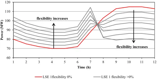
Figure 3.4 Load and reserve scheduling from LSE of type 1 . . . 67

Figure 3.5 Load and reserve scheduling from LSE of type 2 . . . 68

Figure 3.6 Topology of the 6-bus system . . . 77

Figure 3.7 Wind power generation scenarios (6-bus system) . . . 79

Figure 3.8 Analysis of period 4:10 in moderate scenario when contribution of LSEs is neglected. a) without contingencies, b) U2 fails at 4:10, c) transmission line 2 fails at 4:10. Red color: generation and consumption scheduled in the day-ahead market. Green color: generation, consumption and active power flows in moderate scenario. All values are in MW. . . 83

Figure 3.9 Analysis of period 4:10 in moderate scenario when contribution of LSEs is considered. a) without contingencies, b) U2 fails at 4:10, c) transmission line 2 fails at 4:10. Red color: generation and consumption scheduled in the day-ahead market. Green color: generation, consumption and active power flows in moderate scenario. All values are in MW. . . 84

Figure 3.10 Scheduled load of LSE of type 1 connected at bus 18 . . . 86

Figure 3.11 Scheduled load of LSE of type 1 connected at bus 20 . . . 86

Figure 3.12 Energy cost for different values of LSE of type 1 flexibility (C1-A) . . . 87

Figure 3.13 Reserve cost for different values of LSE of type 1 flexibility (C1-A) . . . 87

Figure 3.14 Generation scheduled reserve cost for different costs of LSE of type 1 reserve cost . . . 88

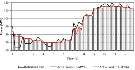
Figure 3.15 Scheduled load of LSE of type 1 and actual consumption in scenario 10 . . 89

Figure 3.16 Baseline load of LSE of type 2 and deployed contingency reserve . . . 89

Figure 4.2 The types of industrial processes . . . 99

Figure 4.3 Topology of the 6-bus system . . . 108

Figure 4.4 Wind power generation scenarios (6-bus system) . . . 110

Figure 4.5 Total system load in the base case and C2 . . . 112

Figure 4.6 Scheduled industrial load . . . 113

Figure 4.7 Industrial load in Low wind production scenario . . . 113

(16)

Figure 4.9 Industrial load in High wind production scenario . . . 114

Figure 4.10 Industrial load reallocation and wind power generation in Moderate scenario 114 Figure 4.11 Baseline industrial load consumption (bus 2) . . . 115

Figure 4.12 Baseline industrial load consumption (bus 19) . . . 116

Figure 4.13 Scheduled wind power and generation side reserves . . . 117

Figure 4.14 Day-ahead energy and reserve cost for different values of wind spillage cost 118 Figure 4.15 Day-ahead wind power scheduling for different values of wind spillage cost . 118 Figure 4.16 Wind spillage in individual scenarios for different values of wind spillage cost 119 Figure 4.17 Cumulative distribution function of cost in different scenarios . . . 119

Figure 4.18 Scheduled industrial load and reserves for industrial load at bus 2 (C1-C) . 122 Figure 4.19 Scheduled industrial load and reserves for industrial load at bus 19 (C1-C) . 122 Figure 4.20 Cumulative distribution function of cost in different scenarios (1500 MW installed wind generation capacity) . . . 124

Figure 4.21 Efficienty frontiers of the examined cases . . . 125

Figure 4.22 Generation side reserve cost for different levels of risk aversion . . . 126

Figure 4.23 Average available wind spillage for different levels of risk aversion . . . 126

Figure 5.2 Load of DRP of type 1 in scenario 12 . . . 147

Figure 5.3 Load of DRP of type 2 in scenario 1 . . . 147

Figure 5.4 Comparison of efficient frontiers: classic vs. the proposed approach . . . 148

Figure 5.5 Wind energy scheduled and expected wind energy spillage . . . 149

Figure 5.6 Day-ahead energy and reserve cost . . . 149

Figure 5.7 Efficient frontiers for different percentages of participation of DRP in reserves 150 Figure 5.8 Efficient frontiers for different values of the load recovery rate . . . 151

Figure 5.9 Similarity index of solution #10 for different values of weight over the ex-pected cost . . . 152

Figure 5.10 Average similarity index of different solutions . . . 154

Figure 5.11 Load of DRP of type 2 at bus 15 in scenario 1 . . . 154

Figure 5.12 Load of DRP of type 2 at bus 18 in scenario 1 . . . 155

Figure 5.13 Efficient frontiers for different values of the cost of the energy not recovered 156 Figure 5.14 Efficient frontiers for different scheduling and deployment costs of DRP reserve157 Figure 5.15 Comparison of efficient frontiers: classic vs. the proposed approach (24 bus system) . . . 158

Figure A.1 Decision variable space and objective function space of the example multi-objective optimization problem . . . 171

Figure A.2 Solution of the multi-objective optimization problem using AUGMECON . 172 Figure B.1 Normalized historical wind farm production . . . 173

Figure B.2 ACF and PACF of the residuals . . . 174

Figure B.3 Histogram of the residuals . . . 174

Figure B.4 Initial set of scenarios . . . 175

Figure C.1 The 24-bus system . . . 177

Figure C.2 10 wind power generation scenarios (Chapter 3) . . . 177

(17)

List of Tables

Table 3.1 Characteristics of the transmission lines (6-bus system) . . . 78

Table 3.2 Technical characteristics of the generating units (6-bus system) . . . 78

Table 3.3 Economic characteristics of the generating units (6-bus system) . . . 78

Table 3.4 System load (6-bus system) . . . 79

Table 3.5 Intra-hour system load (6-bus system) . . . 80

Table 3.6 Scheduled generator output, generation and demand side reserves (MW) . . 81

Table 3.7 Energy and reserve costs for cases C2-A, C2-B and C2-C . . . 90

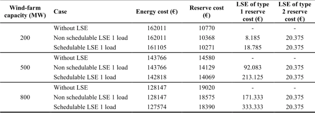
Table 3.8 Energy and reserve costs for different installed capacity of wind farm (C3) . 90 Table 3.9 Computational statistics (6-bus system) . . . 91

Table 3.10 Computational statistics (24-bus system) . . . 91

Table 4.1 Characteristics of the transmission lines (6-bus system) . . . 109

Table 4.2 Technical characteristics of the generating units (6-bus system) . . . 110

Table 4.3 Economic characteristics of the generating units (6-bus system) . . . 110

Table 4.4 System load (6-bus system) . . . 111

Table 4.5 Technical data of industrial processes (6-bus system) . . . 111

Table 4.6 Characteristics of the scenario cost distribution . . . 120

Table 4.7 Technical characteristics of dispatchable processes . . . 121

Table 4.8 Costs for the different cases . . . 121

Table 4.9 Results for different sizes of installed wind farm capacity . . . 124

Table 4.11 Computational statistics - risk neutral problem (24-bus system) . . . 127

Table 4.12 Computational statistics - risk averse problem (24-bus system) . . . 128

Table 5.1 Numbering of efficient solutions . . . 152

Table 5.2 Raking of efficient solutions for different values of weights over the objectives 153 Table 5.3 Decomposition of cost and energy components for different values of cost of energy not recovered . . . 157

Table 5.4 Ranking of efficient solutions for different values of expected cost weight . . 159

Table 5.5 Average similarity index of different solutions (24 bus system) . . . 159

Table C.1 Characteristics of the transmission system . . . 178

Table C.2 Location of generating units . . . 179

Table C.3 Technical data of conventional generators (Chapter 3) . . . 179

Table C.4 Economic data of conventional generators (Chapters 3, 4 and 5) . . . 179

Table C.5 System load (Chapter 3) . . . 180

Table C.6 Probabilities of scenarios (Chapter 3) . . . 180

Table C.7 Technical data of conventional generators (Chapters 4 and 5) . . . 181

Table C.8 System load (Chapters 4 and 5) . . . 182

(18)

Acronyms

4CP Four Coincident Peak

AC Air-conditioner

ACT Air Conditioned Trial

ADRP Automated DR Program

AEMC Australian Energy Market Commission

AEP American Electric Power

AER Australian Energy Regulator

AHU Air Handling Unit

AMI Advanced Metering Infrastructure AML Algebraic Modelling Language

ANEEL Brazilian Electricity Regulatory Agency ARIMA Auto-Regressive Integrated Moving Average

AS Ancillary Services

AUGMECON Augmented Epsilon Constraint (method) BIP Base Interruptible Program

BMS Building Management System

BPDB Bangladesh Power Development Board

CAISO California ISO

CFE Comisión Federal de Electricidad CPP Critical Peak Pricing

CSRP Commercial System Relief Program CVaR Conditional Value-at-Risk

DADRP Day-ahead DR Program

DBP Demand Bidding Program

DLC Direct Load Control

DLRP Distribution Load Relief Program

DM Decision Maker

DOE (U.S.) Department of Energy

DR Demand Response

DRP Demand Response Provider

DRS Demand Reduction Strategy

DSASP Demand Side Ancillary Services Program

DSM Demand Side Management

EDA Electricity of the Azores

EDP Extreme Day Pricing

EDRP Emergency DR Program

EED Energy Efficiency Directive

EMA Energy Market Authority

EMS Energy Management System

ENTSO-E European Network of TSOs for Electricity EPRI Electric Power Research Institute

ERCOT Electric Reliability Council of Texas

(19)

EV Electric Vehicle

FEBELIEC Federation of Beligan Industrial Energy Consumers

FIL Firm Service Level

FPL Florida Power&Light

GAMS General Algebraic Modeling System

HAN Home Area Network

HEMS Home EMS

HVAC Heating Ventilation and Air Conditioning ICT Information and Communications Technology IESO Independent Electricity System Operator (Ontario)

IP Internet Protocol

IR Instantaneous Reserves

ISO Independent System Operator

ISO-NE ISO New England

LMP Locational Marginal Price

LP Linear Programming

LSE Load Serving Entity

MILP Mixed-integer Linear Programming

MISO Midcontinent ISO

MO Market Operator

MOOP Multi-objective Optimization Problem

NAN Neighbourhood Area Network

NEMS National Electricity Market of Singapore

NERC North American Electric Reliability Corporation NIST (U.S.) National Institute of Standards and Technology

NYISO New York ISO

OBMC Optional Binding Mandatory Curtailment OpenADR Open Automated DR

PDPD Peak Day Pricing Program PG&E Pacific Gas&Electric Company

PJM Pennsylvania New Jersey Maryland (Interconnection)

PLC Power Line Communication

PV Photovoltaic

RES Renewable Energy Sources

RTP Real Time Pricing

SCE Souther California Edison SCR Spacial Case Resources

SDGE San Diego Gas&Electric Company SHEP Small Hydroelectric Power Plant SLRP Scheduled Load Reduction Program

SMP System Marginal Price

SOP Standard Offer Program

STOR Short-Term Operating Reserve

TDSP Transmission and Distribution Service Providers

TECO Tampa Electric Company

TOPSIS Technique for Order Preference By Similarity to Ideal Solution

(20)

TSO Transmission System Operator UPS Uninterruptible Power Source

V2G Vehicle-to-Grid

VaR Value-at-Risk

VFD Variable Frequency Drives

WAN Wide Area Network

(21)

Nomenclature

The main notation used in Chapters 3, 4 and 5 is listed below. Other symbols are defined where they first appear. Note that in order to state that a constraint holds ”for every” element of a set, instead of e.g.,∀i ∈ I, for the sake of brevity, ∀i is used, unless strict notation is required to identify the domain of a constraint.

Chapter 3 Sets and indices

b (B(n, nn)) index (set) of transmission lines. Bn

b set of sending nodes of transmission line b. Bnn

b set of receiving nodes of transmission line b.

f (Fi) index (set) of steps of the marginal cost function of unit i. i (I) index (set) of conventional generating units.

j1 (J1) index (set) of LSE of type 1.

j2 (J2) index (set) of LSE of type 2.

n (N ) index (set) of nodes.

Nx

n set of resources of type x∈ {i, j1, j2, r, w} connected to node n.

r (R) index (set) of inelastic loads.

s (Sw) index (set) of scenarios of wind farm w.

t1 (T1) index (set) of time intervals in the first stage of the problem.

t2 (T2) index (set) of time intervals in the second stage of the problem.

w (W ) index (set) of wind farms.

Parameters

Bi,f,t1 size of step f of unit i marginal cost function in period t1 (MW).

Bb,n susceptance of transmission line b (per unit).

Ci,f,t1 marginal cost of step f of unit i marginal cost function in period t1(e/MWh).

C_i,tR,DN

1 offer cost of down spinning reserve by generating unit i in period t1 (e/MWh).

C_jDN,LSE1

1,t1 offer cost of down reserve by LSE of type 1 j1 in period t1 (e/MWh).

C_jDN,LSE2

2,t1 offer cost of down reserve by LSE of type 2 j2 in period t1 (e/MWh).

C_i,tR,N S

1 offer cost of non spinning reserve by generating unit i in period t1(e/MWh).

C_i,tR,U P

1 offer cost of up spinning reserve by generating unit i in period t1 (e/MWh).

C_jU P,LSE1₁_,t₁ offer cost of up reserve by LSE of type 1 j1 in period t1 (e/MWh).

C_jU P,LSE2

2,t1 offer cost of up reserve by LSE of type 2 j2 in period t1 (e/MWh).

D1

r,t1 demand of inelastic load r in period t1 (MW).

D2

r,t2 demand of inelastic load r in period t2 (MW).

DT1

i minimum down time of unit i (h). DT_i2 minimum down time of unit i (min). E_jreq

1 energy requirement of LSE of type 1 j1 (MWh).

fmax

(22)

LCb,t2 transmission line b contingency parameter — 0 if transmission line b is under

contingency in period t2, else 1.

LSE1max

j1,t1 maximum load of LSE of type 1 j1in period t1(MW).

LSE1min

j1,t1 minimum load of LSE of type 1 j1in period t1(MW).

LSE2max

j2,t1 maximum load of LSE of type 2 j2in period t1(MW).

LSE2min_j₂_,t₁ minimum load of LSE of type 2 j2in period t1(MW).

Ncall

j2 maximum number of calls of LSE of type 2 j2.

P_imax maximum power output of unit i (MW). Pmin

i minimum power output of unit i (MW). PW P

w,t2,s power output of wind farm w in period t2 in scenario s (MW).

P_wW P,max maximum amount of wind that may be scheduled in the day-ahead market (MW). RDi ramp down rate of unit i (MW/min).

RUi ramp up rate of unit i (MW/min). SDCi shutdown cost of generating unit i (e). SU Ci startup cost of generating unit i (e). Tdur

j2 maximum duration of contingency reserve provision by LSE of type 2 j2(min).

U Ci,t2 unit i contingency parameter — 0 if transmission line i is under contingency in

period t2, else 1.

U T1

i minimum up time of unit i (h). U T_i2 minimum up time of unit i (min). VLOL

r,t2 cost of involuntary load shedding of inelastic load r in period t2 (e/MWh).

V_w,tspill

2 wind spillage cost of wind from wind farm w in period t2 (e/MWh).

∆T1 length of time interval in the first stage (min). ∆T2 length of time interval in the second stage (min).

λLSE1_j₁_,t₁ utility of LSE of type 1 j1 in period t1 (e/MWh).

λLSE2

j2,t1 utility of LSE of type 2 j2 in period t1 (e/MWh).

πs probability of occurence of wind power scenario s. TN S _{non spinning reserve deployment time (min).} TS _{spinning reserve deployment time (min).}

Variables

bi,f,t1 power output scheduled from the f -th block by unit i in period t1 (MW).

CAi,t2,s additional cost incurring due to a change in the commitment status of unit i in

period t2 in scenario s (e).

fb,t2,s active power flow through transmission line b in period t2 in scenario s (MW).

Lshed

r,t2,s load shed from inelastic load r in period t2 in scenario s (MW).

LSE1DN

j1,t1 total down reserve scheduled from LSE of type 1 j1in period t1(MW).

LSE1DN,load_j

1,t1 down reserve scheduled to balance load deviations from LSE of type 1 j1in period

t1(MW).

LSE1DN,wind_j

1,t1 down reserve scheduled to balance wind deviations from LSE of type 1 j1 in

period t1 (MW).

LSE1U P

j1,t1 total up reserve scheduled from LSE of type 1 j1in period t1(MW).

LSE1U P,load_j

1,t1 up reserve scheduled to balance load deviations from LSE of type 1 j1in period

t1(MW).

LSE1U P,wind_j

1,t1 up reserve scheduled to balance wind deviations from LSE of type 1 j1 in period

(23)

LSE1ac_j₁_,t₂_,s actual consumption of LSE of type 1 j1 in period t2 in scenario s (MW).

LSE1d

j1,t2,s total down reserve deployed from LSE of type 1 j1 in period t2 in scenario

s (MW). LSE1sch

j1,t1 scheduled consumption of LSE of type 1 j1 in period t1 (MW).

LSE1u

j1,t2,s total up reserve deployed from LSE of type 1 j1 in period t2in scenario s (MW).

LSE1d,load_j

1,t2,s down reserve deployed to balance load deviations from LSE of type 1 j1in period

t2in scenario s (MW).

LSE1d,wind_j₁_,t₂_,s down reserve deployed to balance wind deviations from LSE of type 1 j1in period

LSE1u,load_j

1,t2,s up reserve deployed to balance load deviations from LSE of type 1 j1 in period

LSE1u,wind_j

1,t2,s up reserve deployed to balance wind deviations from LSE of type 1 j1 in period

LSE2DN,con_j

2,t1 down reserve scheduled from LSE of type 2 j2 in period t1 (MW).

LSE2U P,con_j

2,t1 up reserve scheduled from LSE of type 2 j2 in period t1 (MW).

LSE2ac

j2,t2,s actual consumption of LSE of type 2 j2 in period t2 in scenario s (MW).

LSE2d,con_j

2,t2,s down reserve deployed from LSE of type 2 j2 in period t2 in scenario s (MW).

LSE2sch_j₂_,t₁ scheduled consumption of LSE of type 2 j2 in period t1 (MW).

LSE2u,con_j

2,t2,s up reserve deployed from LSE of type 2 j2 in period t2 in scenario s (MW).

P_i,tG₂_,s actual power output of unit i in period t2 in scenario s (MW).

Psch

i,t1 power output scheduled for uniti in period t1(MW).

P_w,tW P,S

1 scheduled wind power for wind farm w in period t1 (MW).

RDN_i,t₁ total down spinning reserve scheduled from unit i in period t1 (MW).

RDN,con_i,t

1 contingency down spinning reserve scheduled from unit i in period t1 (MW).

RDN,load_i,t₁ down spinning reserve scheduled to balance load deviations from unit i in period t1(MW).

RDN,wind_i,t

1 down spinning reserve scheduled to balance wind deviations from unit i in period

t1(MW).

RN S

i,t1 total non spinning reserve scheduled from unit i in period t1 (MW).

RN S,con_i,t

1 contingency non spinning reserve scheduled from unit i in period t1(MW).

RN S,load_i,t

1 non spinning reserve scheduled to balance load deviations from unit i in period

t1(MW).

RN S,wind_i,t

1 non spinning reserve scheduled to balance wind deviations from unit i in period

t1(MW).

RU P_i,t₁ total up spinning reserve scheduled from unit i in period t1(MW).

RU P,con_i,t

1 contingency up spinning reserve scheduled from unit i in period t1 (MW).

RU P,load_i,t₁ up spinning reserve scheduled to balance load deviations from unit i in period t1(MW).

RU P,wind_i,t

1 up spinning reserve scheduled to balance wind deviations from unit i in period

t1(MW).

rG

i,f,t2,s reserve deployed from the f -th block of unit i in period t2in scenario s (MW).

rdn_i,t₂_,s total down spinning reserve deployed from unit i in period t2in scenario s (MW).

rdn,con_i,t

2,s contingency down spinning reserve deployed from unit i in period t2in scenario

s (MW). rdn,load_i,t

2,s down spinning reserve deployed to balance load deviations from unit i in period

(24)

rdn,wind_i,t₂_,s down spinning reserve deployed to balance wind deviations from unit i in period t2in scenario s (MW).

rns

i,t2,s total non spinning reserve deployed from unit i in period t2in scenario s (MW).

rns,con_i,t

2,s contingency non spinning reserve deployed from unit i in period t2 in scenario

s (MW). rns,load_i,t

2,s non spinning reserve deployed to balance load deviations from unit i in period t2

in scenario s (MW).

rns,wind_i,t₂_,s non spinning reserve deployed to balance wind deviations from unit i in period t2in scenario s (MW).

rup_i,t

2,s total up spinning reserve deployed from unit i in period t2in scenario s (MW).

rup,con_i,t

2,s contingency up spinning reserve deployed from unit i in period t2 in scenario

s (MW).

rup,load_i,t₂_,s up spinning reserve deployed to balance load deviations from unit i in period t2 in scenario s (MW).

rup,wind_i,t

2,s up spinning reserve deployed to balance wind deviations from unit i in period t2

in scenario s (MW). SDC1

i,t1 shutdown cost of unit i in period t1(e).

SDC_i,t2 ₂_,s shutdown cost of unit i in period t1in scenario s (e).

SU C1

i,t1 startup cost of unit i in period t1(e).

SU C_i,t2 ₂_,s startup cost of unit i in period t1in scenario s (e).

Sw,t2,s wind spilled from wind farm w in period t2 in scenario s (MW).

u1

i,t1 binary variable — 1 if unit i is committed in period t1, else 0.

u2_i,t₂_,s binary variable — 1 if unit i is committed in period t2 in scenario s, else 0.

y1

i,t1 binary variable — 1 if unit i is starting up in period t1, else 0.

y_i,t2₂_,s binary variable — 1 if unit i is starting up in period t2 in scenario s, else 0.

z1

i,t1 binary variable — 1 if unit i is shutting down in period t1, else 0.

z2

i,t2,s binary variable — 1 if unit i is shutting down in period t2in scenario s, else 0.

δn,t2,s binary variable — voltage angle of node n in period t2 in scenario s (rad).

ζLSE2

j2,t2,s binary variable — 1 if LSE of type 2 j2 stops providing contingency reserve in

period t2 in scenario s, else 0.

υLSE2

j2,t2,s binary variable — 1 if LSE of type 2 j2 is providing contingency reserve in

period t2 in scenario s, else 0.

υdn

j2,t2,s binary variable — 1 if LSE of type 2 j2 is providing down contingency reserve

in period t2in scenario s, else 0.

υu_j₂_,t₂_,s binary variable — 1 if LSE of type 2 j2 is providing up contingency reserve in period t2 in scenario s, else 0.

ψLSE2_j₂_,t₂_,s binary variable — 1 if LSE of type 2 j2is called to provide contingency reserve in period t2in scenario s, else 0.

Chapter 4 Sets and indices

b (B(n, nn)) index (set) of transmission lines.

B_bn set of sending nodes of transmission line b. Bnn

(25)

d (D) index (set) of industrial loads.

f (Fi₎ _{index (set) of steps of the marginal cost function of unit i.} g (Gd₎ _{index (set) of groups of processes of industrial load d.} i (I) index (set) of conventional generating units.

j (J ) index (set) of inelastic loads.

Nx

n set of resources of type x∈ {i, j, d, w} connected to node n. p (Pd) index (ordered set) of processes of industry d.

Ph

type set of process types: h = 1 for continuous, h = 2 for interruptible. s (Sw₎ _{index (set) of scenarios of wind farm w.}

t (T ) index (set) of time intervals.

Parameters

amax_p,g,d positive integer — maximum number of available production lines for process p of group g of industrial load d.

amax,h_p,g,d positive integer — maximum number of production lines per hour for process p of group g of industrial load d.

Bi,f,t size of step f of unit i marginal cost function in period t (MW). Bb,n susceptance of transmission line b (per unit).

Ci,f,t marginal cost of step f of unit i marginal cost function in period t (e/MWh). C_i,tR,D offer cost of down spinning reserve by generating unit i in period t (e/MWh). C_i,tR,U offer cost of up spinning reserve by generating unit i in period t (e/MWh). C_i,tR,N S offer cost of non spinning reserve by generating unit i in period t (e/MWh). C_d,tR,D,In offer cost of down reserve by industrial load d in period t (e/MWh).

C_d,tR,U,In offer cost of up reserve by industrial load d in period t (e/MWh).

C_d,tR,N S,In offer cost of non spinning reserve by industrial load d in period t (e/MWh). Dmin

d,t minimum power of industrial load d in period t (MW). DTi minimum down time of unit i (h).

f_bmax maximum capacity of transmission line b (MW). Lj,t demand of inelastic load j in period t (MW). P_imax maximum power output of unit i (MW). Pmin

i minimum power output of unit i (MW). Pline

p,g,d power of production line of process p of group g of industrial load d (MW). PW P

w,t,s power output of wind farm w in scenario s in period t (MW).

P_w,tW P,max maximum amount of wind that may be scheduled in the day-ahead market (MW). RDi ramp down rate of unit i (MW/min).

RUi ramp up rate of unit i (MW/min). SDCi shutdown cost of generating unit i (e). SU Ci startup cost of generating unit i (e).

TN S _{non spinning reserve deployment time (min).} TS spinning reserve deployment time (min).

T_p,g,dc,max maximum completion time of process p of group g of industrial load d (h). T_p,g,dg,max maximum time interval between processes p and p + 1 of group g of industrial

(26)

T_p,g,dg,min minimum time interval between processes p and p + 1 of group g of industrial load d (h).

U Ti minimum up time of unit i (h).

VLOL _{cost of involuntary load shedding for inelastic loads (}_e/MWh). Vs _{wind spillage cost (e/MWh).}

α confidence level (CV aR calculation). β weighting factor (CV aR calculation). ∆T length of time interval (min).

λD

d,t utility of industrial load d in period t (e/MWh). πs probability of occurence of wind power scenario s.

Variables

ap,g,d,t integer variable — number of production lines scheduled from process p of group g of industrial load d in period t.

a2_p,g,d,t,s integer variable — number of production lines scheduled from process p of group g of industrial load d in period t in scenario s.

adown_p,g,d,t integer variable — number of production lines scheduled from process p of group g of industrial load d in period t to provide down reserves.

adown,rt_p,g,d,t,s integer variable — number of production lines that are used to deploy down reserves from process p of group g of industrial load d in period t in scenario s. ans

p,g,d,t integer variable — number of production lines scheduled from process p of group g of industrial load d in period t to provide non spinning reserves.

ans,rt_p,g,d,t,s integer variable — number of production lines that are used to deploy non spinning reserves from process p of group g of industrial load d in period t in scenario s.

aup_p,g,d,t integer variable — number of production lines scheduled from process p of group g of industrial load d in period t to provide up reserves.

aup,rt_p,g,d,t,s integer variable — number of production lines that are used to deploy up reserves from process p of group g of industrial load d in period t in scenario s. bi,f,t power output scheduled from the f -th block by unit i in period t (MW). CV aR conditional value-at-risk (e).

fb,t,s active power flow through transmission line b in period t in scenario s (MW). Lshed

j,t,s load shed from inelastic load j in period t in scenario s (MW). P_i,t,sG actual power output of unit i in period t in scenario s (MW).

P_d,t,sind,C actual power consumption of industrial load d in period t in scenario s (MW). P_d,tind,S scheduled consumption of industrial load d in period t (MW).

P_p,g,d,t,spro,C actual power consumption of process p of group g of industrial load d in period t in scenario s (MW).

P_p,g,d,tpro,S scheduled consumption of process p of group g of industry d in period t (MW). PS

i,t power output scheduled for unit i in period t (MW). P_w,tW P,S scheduled wind power for wind farm w in period t (MW). RD

i,t down spinning reserve scheduled from unit i in period t (MW). RD,ind_d,t down reserve scheduled from industrial load d in period t (MW).

RD,pro_p,g,d,t scheduled down reserve from process p of group g of industrial load d in period t (MW).

(27)

rD,pro_d,g,p,t,s down reserve deployed from the process p of the group g of industrial load d in period t in scenario s (MW).

rD

i,t,s down spinning reserve deployed from unit i in period t in scenario s (MW). rG

i,f,t,s reserve deployed from the f -th block of unit i in period t in scenario s (MW). RN S

i,t non spinning reserve scheduled from unit i in period t (MW).

RN S,ind_d,t non spinning reserve scheduled from industrial load d in period t (MW). RN S,pro_p,g,d,t scheduled non spinning reserve from process p of group g of industrial load d in

period t (MW).

rN S,pro_d,g,p,t,s non spinning reserve deployed from the process p of the group g of industrial load d in period t in scenario s (MW).

rN S_i,t,s non spinning reserve deployed from unit i in period t in scenario s (MW). RU

i,t up spinning reserve scheduled from unit i in period t (MW). RU,ind_d,t up reserve scheduled from industrial load d in period t (MW).

RU,pro_p,g,d,t scheduled up reserve from process p of group g of industrial load d in period t (MW).

rU,pro_d,g,p,t,s up reserve deployed from the process p of the group g of industrial load d in period t in scenario s (MW).

rU_i,t,s up spinning reserve deployed from unit i in period t in scenario s (MW). Sw,t,s wind spilled from wind farm w in period t in scenario s (MW).

u1_i,t binary variable — 1 if unit i is committed during period t, else 0. u2

i,t,s binary variable — 1 if unit i is committed during period t in scenario s, else 0. y1

i,t binary variable — 1 if unit i is starting up in period t, else 0.

y_i,t,s2 binary variable — 1 if unit i is starting up in period t in scenario s, else 0. z1

i,t binary variable — 1 if unit i is shutting down in period t, else 0.

z2_i,t,s binary variable — 1 if unit i is shutting down in period t in scenario s, else 0. δn,t,s voltage angle of node n in period t in scenario s (rad).

ζ1

p,g,d,t binary variable — 1 if process p of group g of industrial load d is terminated in period t, else 0.

ζ2

p,g,d,t,s binary variable — 1 if process p of group g of industrial load d is terminated in period t in scenario s, else 0.

ηs non negative auxiliary variable (CV aR calculation) (e). ξ auxiliary variable (CV aR calculation) (e).

υ1

p,g,d,t binary variable — 1 if process p of group g of industrial load d is in progress in period t, else 0.

υ2_p,g,d,t,s binary variable — 1 if process p of group g of industrial load d is in progress in period t in scenario s, else 0.

ψ1_p,g,d,t binary variable — 1 if process p of group g of industrial load d is beginning in period t, else 0.

ψ2

p,g,d,t,s binary variable — 1 if process p of group g of industrial load d is beginning in period t in scenario s, else 0.

Chapter 5 Sets and indices

(28)

B_bn set of sending nodes of transmission line b. Bnn

b set of receiving nodes of transmission line b.

f (Fi₎ _{index (set) of steps of the marginal cost function of unit i.} i (I) index (set) of conventional generating units.

IN S _{set of generating units capable of providing non spinning reserves.} j (J ) index (set) of loads.

J0 _{set of inelastic loads.}

J1 set of demand response providers of type 1. J2 _{set of demand response providers of type 2.}

N_nx set of resources of type x∈ {i, j, w} connected to node n. s (Sw₎ _{index (set) of scenarios of wind farm w.}

t (T ) index (set) of time intervals.

Parameters

Bb,n susceptance of transmission line b (per unit).

Bi,f,t size of step f of unit i marginal cost function in period t (MW).

C_i,tG,D offer cost of up spinning reserve by generating unit i in period t (e/MWh). C_i,tG,U offer cost of down spinning reserve by generating unit i in period t (e/MWh). C_i,tG,N S offer cost of non spinning reserve by generating unit i in period t (e/MWh). C_j,tDRP,U offer cost of load reduction scheduling from demand j in period t (e/MWh). CG

i,f,t marginal cost of step f of unit i marginal cost function in period t (e/MWh). cDRP,U_j,t cost of load reduction deployment from demand j in period t (e/MWh). Dj,t nominal load of demand j in period t (MW).

DTi minimum down time of unit i (h).

f_bmax maximum capacity of transmission line b (MW). Nin

j maximum number of interruptions of demand j. Pmax

i maximum power output of unit i (MW). P_imin minimum power output of unit i (MW). PW,max

w maximum amount of wind that may be scheduled in the day-ahead market (MW). Pw,t,sW P power output of wind farm w in scenario s in period t (MW).

p maximum participation of demand side resources in reserves (%). RDRP,U,m_j minimum load reduction of demand j (MW).

RDi ramp down rate of unit i (MW/min). RDDRP

j load pickup rate of demand j (MW/min). RUi ramp up rate of unit i (MW/min). RUDRP

j load drop rate of demand j (MW/min). SDCi shutdown cost of generating unit i (e). SU Ci startup cost of generating unit i (e).

TN S _{non spinning reserve deployment time (min).} T_jrec duration of the load recovery period (h). TS _{spinning reserve deployment time (min).} U Ti minimum up time of unit i (h).

VEN S

j cost of energy not served/not recovered of load j (e/MWh). VS _{wind spillage cost (}_e/MWh).

(29)

α confidence level (CV aR calculation). β weighting factor (CV aR calculation).

γj load recovery rate with respect to load reduction of load j (%). ∆T length of time interval (min).

ξD

j,t maximum downward demand modification of demand j in period t (%). ξ_j,tU maximum upward demand modification of demand j in period t (%). πs probability of occurrence of wind power scenario s.

Variables

bi,f,t power output scheduled from the f -th block by unit i in period t (MW). CV aR conditional value-at-risk (e).

DA

j,t,s actual consumption of demand j in period t in scenario s (MW). EN Rj,s energy of demand j not recovered in scenario s (MWhh).

fb,t,s active power flow through transmission line b in period t in scenario s (MW). Lshed_j,t,s load shed from inelastic load j in period t in scenario s (MW).

PG

i,t,s actual power output of unit i in period t in scenario s (MW). P_i,tsch power output scheduled for unit i in period t (MW).

P_w,tW,sch scheduled wind power from wind farm w in period t (MW). RDRP,D_j,t load recovery scheduled from demand j in period t (MW). RDRP,U_j,t load reduction scheduled from demand j in period t (MW). RG,D_i,t down spinning reserve scheduled from unit i in period t (MW). RG,N S_i,t non spinning reserve scheduled from unit i in period t (MW). RG,U_i,t up spinning reserve scheduled from unit i in period t (MW). rDRP,d_j,t,s load recovery of demand j in period t in scenario s (MW). rDRP,u_j,t,s load reduction of demand j in period t in scenario s (MW). rG

i,f,t,s reserve deployed from the f -th block of unit i in period t in scenario s (MW). rG,d_i,t,s down spinning reserve deployed from unit i in period t in scenario s (MW). rG,ns_i,t,s non spinning reserve deployed from unit i in period t in scenario s (MW). rG,u_i,t,s up spinning reserve deployed from unit i in period t in scenario s (MW). Sw,t,s wind spilled from wind farm w in period t in scenario s (MW).

u1

i,t binary variable — 1 if unit i is committed during period t, else 0.

u2_i,t,s binary variable — 1 if unit i is committed during period t in scenario s, else 0. uDRP,d_j,t,s binary variable — 1 if demand j is recovering in period t in scenario s. uDRP,u_j,t,s binary variable — 1 if demand j is curtailed in period t in scenario s. y1

i,t binary variable — 1 if unit i is starting up in period t, else 0. y2

i,t,s binary variable — 1 if unit i is starting up in period t in scenario s, else 0. z1

i,t binary variable — 1 if unit i is shutting down in period t, else 0. z2

i,t,s binary variable — 1 if unit i is shutting down in period t in scenario s, else 0. δn,t,s voltage angle of node n in period t in scenario s (rad).

ηs non negative auxiliary variable (CV aR calculation) (e). κj,t,s auxiliary variable used to linearize load recovery (MW). ξ auxiliary variable (CV aR calculation) (e).

(30)

Chapter 1

Introduction

1.1 Thesis Motivation: Challenges and Opportunities Under

Large-Scale Penetration of Renewable Energy Sources

It is widely recognized that Renewable Energy Sources (RES) are likely to represent a significant portion of the production mix in many power systems around the world, a trend expected to be increasingly followed in the coming years [1]. There are two main reasons that have motivated the adoption of RES:

1. Environmental issues. Concerns regarding the climate change have led the international community to take actions in order to control the greenhouse gas emissions. The fossil-fuel electricity sector is a major contributor to environmental degradation and therefore, increasing the share of RES is perceived as an environmentally friendly alternative in order to achieve the carbon footprint reduction targets.

2. Scarcity and increased cost of conventional fuels. Many countries and regions rely heavily on the import of external energy resources and especially oil. An apt example of this is the case of the Canary Islands, the electricity generation of which depended by 94% on imported fuels in 2010 [2]. Similarly, Cyprus uses almost exclusively heavy fuel oil and diesel for electricity generation [3]. The price of imported fuels is in turn dependent on geopolitical factors and transportation costs. These issues are likely to contribute to the electricity price volatility. For example, the cost of electricity for residential and commercial end-users was approximately 31 cents per kWh in September 2010, 40 cents per kWh in December 2012, and 42 cents per kWh in the third quarter of 2013 in American Samoa [4]. This increase in the price of electricity was mainly caused by the high and variable cost of fuel per barrel. Given that providing low-cost electricity is essential for the economic development of a country, such an increase in the electricity prices may prove detrimental. On the other hand, there are many autochthonous energy sources that may be used according to the specific needs and peculiarities of each system in order to mitigate imported fuel dependence and to diversify the production mix.

However, despite the potential economic and environmental benefits that arise from the integration of these resources into the power system, large-scale integration of RES leads to additional problems due to the fact that their production is highly volatile and unpredictable. Although leading RES technologies such as wind and solar generation are mature and able to compete with conventional power plants, they are associated with significant variability due to their intrinsically stochastic nature. Wind and solar production depend on wind speed and irradiation values, which in turn fluctuate according to weather changes and spatial characteristics. As a result, instantaneous,

(31)

seasonal and yearly fluctuations affect the generation output of RES. The integration of high levels of dispatchable resources in power systems and especially in relatively small sized, non-interconnected systems such as the insular ones, poses operational and economic challenges that need to be addressed. The magnitude of the problem depends on the penetration of RES in the production mix, while its mitigation is reflected on the “flexibility” of the power system.

The variable production from RES affects the operation of conventional generators [5],[6],[7]. Under high levels of penetration conventional units are likely to operate in a suboptimal commitment and dispatch. Fluctuation of RES output power leads to cycling of conventional units and shortens the life of their turbines, while causing increased generation costs. The emission reduction potential is also suppressed. Furthermore, reserve needs are increasing with the penetration of RES and especially ramping requirements (load following) because of the uncorrelated variation of wind generation and load demand. For instance, a case study for the power system of Cyprus [8] concluded that the available reserve capacity is not adequate to balance the real-time fluctuations of wind, while higher penetration of wind power generation would further constrain the downward ramping capability of the system due to the part loading of generators. This example reveals another challenge for the system stemming from the increasing penetration of RES: the inability of conventional generators to boundlessly reduce their output when the non-dispatchable RES production is high. Typically, diesel-fired generators have a minimum output limit of 30% of their installed capacity. Forcing a load following unit to shut down in order to retain the generation and demand balance may compromise the longer-term reliability of the power system. Thus, to avoid such a deficit in the inertia of the system, RES generation is normally curtailed instead of switching off synchronous generators, at the expense of economic losses [9]. The penetration of RES may also affect voltage stability because power sources such as fixed-speed induction wind turbines and PV converters have limited reactive power control. Surely, additional operational reserves (spinning or non-spinning) are required. Apart from frequency regulation, load-forecasting error, sudden changes (ramps) in the production of RES units, forced or scheduled equipment outages need also to be confronted. To deal with these issues adequate generation or demand side capacity should be kept.

Motivated by the increasing penetration of RES and especially wind power generation in power systems, as well as by the operational problems that have been briefly discussed, this thesis deals with the development of reserve mechanisms that directly incorporate several types of demand side resources in order to cope with the uncertainty of RES production. Prior to delving into the investigation of several aspects of the participation of demand side resources in the power system operations and presenting relevant mathematical models, this introductory chapter aims at providing an overview of the necessary framework of the thesis. First, a short overview of RES based production technologies and basic definitions regarding the participation of the demand side and electricity markets are presented in Sections 1.2, 1.3 and 1.4 respectively. Then, the necessary background on the methodology utilized in this thesis is briefly introduced in Section 1.5. Finally, the research questions together with the novel contributions of this thesis are listed in Section 1.6. The chapter concludes by outlining the structure of the thesis in Section 1.7.

Reserve services provision by demand side resources in systems with high renewables penetration using stochastic optimization

UNIVERSIDADE DA BEIRA INTERIOR

Engenharia

Reserve services provision by demand side

resources in systems with high renewables

penetration using stochastic optimization

Nikolaos Paterakis

Tese para obtenção do Grau de Doutor em

Engenharia e Gestão Industrial

(3º ciclo de estudos)

Orientador: Prof. Doutor João Paulo da Silva Catalão

(Universidade da Beira Interior)

Coorientador: Prof. Doutor Anastasios G. Bakirtzis

(Aristotle University of Thessaloniki)

UNIVERSITY OF BEIRA INTERIOR

Engineering

Reserve services provision by demand side

resources in systems with high renewables

penetration using stochastic optimization

Nikolaos Paterakis

Thesis submitted in fulfillment of the requirements for the degree of

Doctor of Philosophy in

Industrial Engineering and Management

(3

cycle of studies)

Supervisor: Prof. Dr. João Paulo da Silva Catalão

(University of Beira Interior)

Co-supervisor: Prof. Dr. Anastasios G. Bakirtzis

(Aristotle University of Thessaloniki)

Acknowledgments

Resumo

Palavras-chave

Abstract

Keywords

Contents

List of Figures

List of Tables

Acronyms

Nomenclature

Chapter 3

Sets and indices

Parameters

Variables

Chapter 4

Sets and indices

Parameters

Variables

Chapter 5

Sets and indices

Parameters

Variables

Chapter 1

Introduction

1.1 Thesis Motivation: Challenges and Opportunities Under

Large-Scale Penetration of Renewable Energy Sources

_{cycle of studies)}