doi: 10.1590/0101-7438.2017.037.01.0193
A COMPARATIVE STUDY OF STOCHASTIC QUADRATIC PROGRAMMING AND OPTIMAL CONTROL MODEL IN PRODUCTION-INVENTORY
SYSTEM WITH STOCHASTIC DEMAND
Ali Khaleel Dhaiban
Received October 11, 2016 / Accepted March 24, 2017
ABSTRACT.This study compares the optimal control model and stochastic quadratic programming (SQP) model of a production-inventory system. A single product, without shortage in the case of a periodic-review policy with stochastic demand and deterioration rate as a function of time, is discussed. The items are sub-jected to deterioration via storage and the inventory goal level as a function of production. Demand is represented by a stochastic differential equation, converted to a stochastic constraint, and then to a de-terministic constraint. We derive the optimality conditions of optimal control model and formulate three models of SQP. The effect of stochastic demand on the production rate and inventory level is then illus-trated. Our numerical results appear to suggest that control of inventory level is better in the case of SQP. Furthermore, the total cost is similar in the three models of SQP – despite a difference in production rates and inventory levels.
Keywords: optimal control, production-inventory system, stochastic quadratic programming.
1 INTRODUCTION
Production planning needs to take many factors into account, in order to realize maximum prof-itability. Inventory, which is one of these factors, has emerged in the last decade. The balance between production process and inventory level, to hedge demand with the lowest cost, is very important in any production-inventory system. Many mathematical models, such as optimal con-trol and mathematical programming, have been developed to deal with this system. Production-inventory systems face many problems, such as the life age of products during storage and the determination of exogenous demand. In practice, demand is often not specified, as it relies on customers and competition. Therefore, a production-inventory system with stochastic demand was developed.
Numerous researchers have investigated inventory systems with stochastic demand. Kleywegt et al. (2004), Mubiru (2014) and Feng et al. (2015) have formulated the Markov decision process
to describe stochastic demand. Kleywegt et al. (2004) discussed a routing problem, and pro-posed a method to solve that problem. The target was to minimize the total cost by determining the replenishment amount, and selecting a suitable method of transportation. Mubiru (2014) de-tailed the order policy on milk powder in supermarkets to minimize the total cost of ordering and holding stock, in addition to the shortage cost. The optimal policy of replenishment, and its structure in inventory systems with multiple products, neglect lead time, and discount rate, was investigated by Feng et al. (2015). He proposed a policy that clarified the stochastic demand effect on the optimal policy structure. Levi et al. (2007) considered two problems of stochastic inventory; periodic-review and lot-sizing, with single item and location. The goal was to balance between the costs of excess inventory and backlog demand, in order to minimize total costs. Hurley et al. (2007) extended the Levy model by proposing two policies to determine the lower and upper bounds of inventory depending on the techniques of cost-balancing and myopic-like. Wanke (2010) investigated two rules of demand allocation with lead time and demand as random variables that follow a normal distribution. He compared two rules based on safety stock, total stock and total cost. Two optimization models with defective items and normal distribution of demand; fuzzy and intuitionistic fuzzy were investigated by Banerjee (2011). The author dis-cussed the chance-constraints model with multi objectives and demand that adhered to uniform and exponential distributions. Also, using two cases of defective items, Bhowmick & Samanta (2012) addressed the inventory model with a single period, partial backlogging, and stochastic demand, depending on the price to determine the order quantity. Kim & Jeong (2012) developed a mathematical model of buyer-supplier with a single item, demand normally distributed, and periodic-review to find the optimal length of cycle. Demand, as a simple Poisson process in the continuous- review of the multistage inventory system, was discussed by Hu & Yang (2014). They modified a policy of echelon(r,Q)replenishment, for any stage, based on previous stages, and clarified the results of a multi-stage system based on a two-stage system’s results. The works of Kumar et al. (2011), Castellano (2015), Mubiru (2015) and Soysal (2016), covered many aspects of this topic.
Another mathematical model, which was used to plan a production-inventory system, is stochas-tic mathemastochas-tical programming. Tarim et al. (2006) developed stochasstochas-tic linear programming with a discrete distribution of demand and scenario trees for stochastic constraints to minimize the expected total cost of shortage and scrap in an inventory system. Also with stochastic linear programming, Zhang et al. (2006) applied the inventory system to fashion production with a sin-gle period, multiple retailers and stocking echelons; where the first echelon was for raw materials and finished goods were the last echelon. Rossi et al. (2007) studied the replenishment cycle in a production-inventory system with multiple periods, normal distribution of demand, and shortage. The paper took into account the four fixed costs of holding, procurement, ordering, and short-age. A stochastic demand modelled as a scenario tree, such as the one in Tarim et al. (2006), with uncertainty in the equality of the raw materials, multiple periods, and multiple products in sawmill production, was addressed by Kazemi Zanjani et al. (2010). Dogru et al. (2010) and Reiman & Wang (2015) have considered an assemble system with multiple components that was used to assemble multiple products with demand as a compound Poisson process and fixed lead time of component replenishment. They developed two-stage stochastic programming to mini-mize inventory total cost. The effect of risk-pooling on the inventory management of chemical complexes was clarified by You & Grossmann (2011). They formulated an inventory model as mixed-integer nonlinear to determine the optimal rates of feedstocks purchase, production, and inventory, as well as the sale of chemicals. Furthermore, with a mixed-integer but linear model, Chotayakul & Punyangarm (2016) addressed the lot-sizing model using cost, capacity, and time of production: in addition to time and cost of setup, based on the machines used.
Our model contributes knowledge to the literature in several ways. The main contribution clarifies the difference of inventory control according to the two models i.e., optimal control and SQP. This is followed by dealing with deteriorating items in the inventory system, by formulating an SQP model. This is in addition to inventory goal level, as a function of production rather than being a constant, which has been addressed by most previous studies. The last step addresses optimal control using stochastic demand, by developing an optimal control model with equivalent deterministic demand, rather than a stochastic optimal control.
This paper is organized in the following order. Section 2.1 will introduce the notations and as-sumptions involved in the optimal inventory model. Section 2.2 will illustrate the stochastic de-mand. Sections 2.3 and 2.4 will discuss the formulation of the optimal control model and the derivation of the optimality conditions of the periodic-review system. Section 2.5 will detail the SQP model. Section 3 will illustrate the results of the two aforementioned models. The final section will summarize our findings and suggest future researches.
2 MATERIALS AND METHODS
2.1 Notations and Assumptions Involved In the Model 2.1.1 Notations
T = The length of the planning horizon(T >0). Y(t) = The inventory level at timet.
N(t) = The production rate at timet.
D(t) = The stochastic demand rate for the production at timet. D(0) = The initial demand.
δ(t) = The deterioration rate, which depends on the time.
ˆ
y(t) = The inventory goal level, which depends on the production.
ˆ
n(t) = The production goal rate. Y(0) = The initial inventory level.
h = A penalty is incurred when the inventory level deviates from its goal level(h >0).
k = A penalty is incurred when the total production rate to deviate from its goal rate(k>0).
2.1.2 Assumptions
We took into account the following:
1. A firm can produce a certain product, sell some, and stack the rest in a warehouse.
2. The stochastic demand rate.
3. The firm has set an inventory goal level and a production goal rate.
4. Production rates are positive to satisfy demand and achieve a specific level of inventory.
5. No shortage and items are subjected to deterioration through storage.
6. Neglect lead time.
2.2 The Stochastic Demand
Previous studies that dealt with inventory system have taken into account the many types of de-mand; for example, stochastic demand (Mubiru, 2014; Feng et al., 2015), demand as a compound Poisson process (Dogru et al., 2010; Reiman & Wang, 2015) and demand depend on the return products (Raupp et al., 2015). In this study, the demand is represented by the following stochastic differential equation (SDE) (Kiesm¨uller, 2003; Ouaret et al., 2011; Yi et al., 2013):
d D(t)=µdt+σdβ(t) (1)
where
µ = The drift coefficient (constant).
σ = The diffusion coefficient (constant).
The solution of the Eq. (1) is as follows (Wiersema, 2008):
t
0
d D(s)=
t
0
µds+
t
0
σdβ(s)
D(t)−D(0)=µ(t−0)+σ{β(t)−β(0)} (2)
D(t)=D(0)+µt+σβ(t)
Eq. (2) includes two parts; the first part is deterministic D(0)+µt and the second part is a random variableβ(t)that follows a normal distribution with mean zero and variancet.
According to Karki et al. (2014), the stochastic constraint (2) can be converted to a deterministic constraint using the median ofβ(t). In normal distribution the median is equal to the mean, which means that the median is equal to zero.
D(t)=D(0)+µt (3)
Eq. (3) is used in the optimal control model and the quadratic programming model that is equiv-alent to the SQP model.
Another case to the SQP is rewriting Eq. (2) as a chance constraint by considering the Brownian motion as a b vector in the mathematical programming:
D(t)=D(0)+µt+σβ(t)
D(t)−D(0)−µt
σ =β(t)
Pr
D(t)
−D(0)−µt
σ ≥β(t)
≥ pt (4)
or
Pr
D(t)
−D(0)−µt
σ ≤β(t)
≥ pt (5)
wherepis the success probability.
If p = 0.99, it means that the constraint will be achieved with only one percentage of failure (Pr´ekopa, 2013). According to Shapiro & Dentcheva (2014), the deterministic constraint that is equivalent to the stochastic constraint (4) is as follows:
Pr
D(t)
−D(0)−µt−0
σ√t ≤
β(t)−0
√
t
≥ pt
∅
D(t)−D(0)−µt
σ√t
≥ pt
(6)
Eq. (6) can be written as follows:
D(t)≥ D(0)+µt+σ√t ∅−1(pt) (7)
where∅−1(·)is the inverse of CDF of standard normal distribution, and it is taken directly from the standard normal distribution table.
In the same manner, the deterministic constraint that is equivalent to the stochastic constraint (5) is as follows:
1−∅ D(t)
−D(0)−µt
σ√t
≥ pt
D(t)≤D(0)+µt+σ√t ∅−1(1−pt)
(8)
2.3 Optimal control model
The objective function can be expressed as the quadratic form to minimize (Sethi & Thompson, 2000):
2J =
T−1
t=0
h{Y(t)− ˆy(t)}2+k{N(t)− ˆn(t)}2 (9)
subject to the state equation
Y(t)=N(t)−D(t)−δ(t)Y(t); t=0, . . . ,T −1 (10)
and positive constraint
N(t) >0; t =0,1, . . . ,T −1 (11)
with initial and terminal conditions
Y(0)=y0
λ(T)=0
whereY(t)=Y(t+1)−Y(t)is called the difference operator.
2.4 Optimality Conditions and Solution of the Model
Many pervious works have dealt with the inventory goal level as a constant, and in this paper, it is a function of production:
ˆ
y(t+1)=ϕnˆ(t); t =0, . . . ,T −1; 0< ϕ <1
ˆ
y(0)= ˆy0
(12)
Eq. (12) depends on the state variableY(t), and its measured at the beginning periodt, while during the period, the control variableN(t)is determined.
From the state equation (10), the goals of production and inventory are given by:
Substituting Eq. (12) into Eq. (13) yields:
ˆ
n(t)= D(t)
1−ϕ −
1−δ(t)
1−ϕ yˆ(t); t =0, . . . ,T −1 (14)
The Lagrangian function is:
L=
T−1
t=0
−1
2
h{Y(t)− ˆy(t)}2+k{N(t)− ˆn(t)}2
+ T−1
t=0
λ(t+1)
×
N(t)−D(t)−δ(t)Y(t)−Y(t+1)+Y(t)
+ T−1
t=0
Z(t)N(t).
(15)
A Hamiltonian function defined as:
H(t)= −1
2
h{Y(t)− ˆy(t)}2+k{N(t)− ˆn(t)}2
+λ(t+1)N(t)−D(t)−δ(t)Y(t);t =0, . . . ,T −1
(16)
We can write Eq. (15) as follow:
L =
T−1
t=0
{H(t)−λ(t+1)(Y(t+1)−Y(t))} +
T−1
t=0
Z(t)N(t) (17)
Lagrange multiplierZ(t)satisfy the complementary slackness conditions:
Z(t)≥0; Z(t)N(t)=0. (18)
From Eqs. (11) and (18), we get:
Z(t)=0. (19)
Equations (11 & 16) are concave in N(t), so Eqs. (16 & 18) are the necessary and sufficient conditions for maximizing the Hamiltonian problem.
Now, differentiate Eq. (17) with respect toY(t)yields:
λ(t)=h{Y(t)− ˆy(t)} +λ(t+1)δ(t);t =0, . . . ,T−1 (20)
Differentiate Eq. (17) with respect toN(t), yields:
N(t)= ˆn(t)+1
kλ(t+1);t =0,1, . . . ,T −1 (21)
Substituting Eqs. (13 & 21) into Eq. (10), yields:
Y(t)= ˆy(t+1)− ˆy(t)−δ(t){Y(t)− ˆy(t)} +1
From Eqs. (20 & 22), we obtained on the following system of difference equations
Y(t)= −δ(t){Y(t)− ˆy(t)} +1
kλ(t+1);t =0, . . . ,T −1
λ(t)=h{Y(t)− ˆy(t)} +λ(t+1)δ(t);t =0, . . . ,T−1 ⎫ ⎬
⎭
(23)
This equations system (23) can be solved numerically by using Excel with initial condition Y(0)=y0and the terminal conditionλ(T)=0, and then find the production rate from Eq. (21).
2.5 Stochastic Quadratic Programming (SQP) Formulation
In this section, we formulate the SQP problem with quadratic cost function subjected to equality and inequality linear and stochastic constraints (Dost´al, 2009).
The objective function is represented by the quadratic form to minimize penalties are incurred when the inventory level and production rates deviate from its goals. The objective function is similar to the objective function of the optimal control, which means Eq. (9). The constraints are as follow:
1. The inventory level constraints are:
Y(t+1)−N(t)+D(t)− {1−δ(t)}Y(t)=0;t=0, . . . ,T−1 (24)
Eq. (24) represents the inventory levels, which is equal to the production, subtract demand and deterioration.
2. The stochastic demand constraint represents three cases, which means three models of SQP. The first model with Eq. (2), the second model with Eq. (4), and the last model with Eq. (5).
3. Assuming the initial demand constraint is:
D(0)=100 (25)
4. Inventory goal level constraints are:
ˆ
y(t+1)−ϕnˆ(t)=0; t =0, . . . ,T −1
ˆ
y(0)− ˆy0=0
(26)
Y(t)− ˆy≥0; t =0, . . . ,T −1; yˆ >Y(0)
ˆ
y−Y(t)≥0; t=0, . . . ,T −1; yˆ <Y(0)
⎫ ⎬
⎭
(27)
5. The initial inventory level constraint is:
Y(0)=y0 (28)
6. Production goal rate constraints that are similar to Eq. (14):
ˆ
n(t)− D(t)
1−ϕ +
1−d(t)
1−ϕ yˆ(t)=0; t =0, . . . ,T −1 (29)
7. Production rate constraints are:
N(t)− ˆn(t)≥0; t =0,1, . . . ,T −1
N(t) >0; t =0,1, . . . ,T −1
⎫ ⎬
⎭
(30)
Eq. (30) leads to minimize the deviation of production rate from its goals.
8. Deterioration constraint, which is equal to the function of time, is:
δ(t)−0.03t =0; t =0, . . . ,T −1 (31)
To find a solution of the SQP models, we must replace the stochastic demand constraints by its equivalent deterministic constraints. Therefore, Eq. (2) replaced by Eq. (3), Eq. (4) replaced by Eq. (7), and Eq. (5) replaced by Eq. (8).
By assumingpt=0.99, it yields:
∅−1(0.99)=2.323
∅−1(0.01)= −2.323
From Eqs. (7 & 8), we get:
D(t)≥ D(0)+µt+σ√t∗2.323; t=1, . . . ,T−1 (32)
D(t)≤ D(0)+µt+σ√t∗ −2.323; t =1, . . . ,T−1 (33)
3 RESULTS AND DISCUSSION
Consider an inventory system with the following parameter valuesy0 = 10 item; yˆ(0) = 5; T =5 weaks;k=25$;h=10$;ϕ=0.2;δ(t)=0.03t;µ=25;σ =10.
3.1 Solution of the optimal control model
By using the goal seek function in Excel, we find the solution of the system (23):
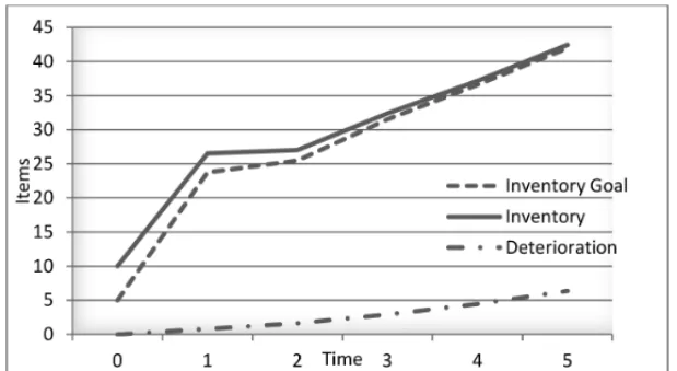
Figure 1– The inventory level, according to the optimal control model.
Figure 2– The production rate, according to the optimal control model.
Table 1– Solution of the optimal control model.
M.V. Time
0 1 2 3 4 5
Y 10.00 26.53 27.03 32.40 37.16 42.46 ˆ
y 5.00 23.75 25.49 31.51 36.58 41.95 ˆ
n 118.75 127.45 157.55 182.91 209.76 N 116.53 126.30 156.98 182.68 209.76 δY 0.00 0.80 1.62 2.92 4.46 6.37
λ –105.61 –55.61 –28.71 –14.11 –5.76 0.00
found by Sethi & Thompson (2000) and Pan & Li (2014), which means inventory level and production rates as close as to their goals over time, regardless a difference in the assumptions of the models.
The following can be deduced from Table 1:
1. Depending on the value of penalty costs, the convergence between the production rate and its goal is more than the convergence between the inventory level and its goal.
2. The production rate is equal to its goal in the fourth week, due to the terminal condition of
λ(5)=0.
3. The total cost is 264$.
3.2 Solution of the SQP model
To find the solution of the SQP problem, we use MatLab (version 8.5).
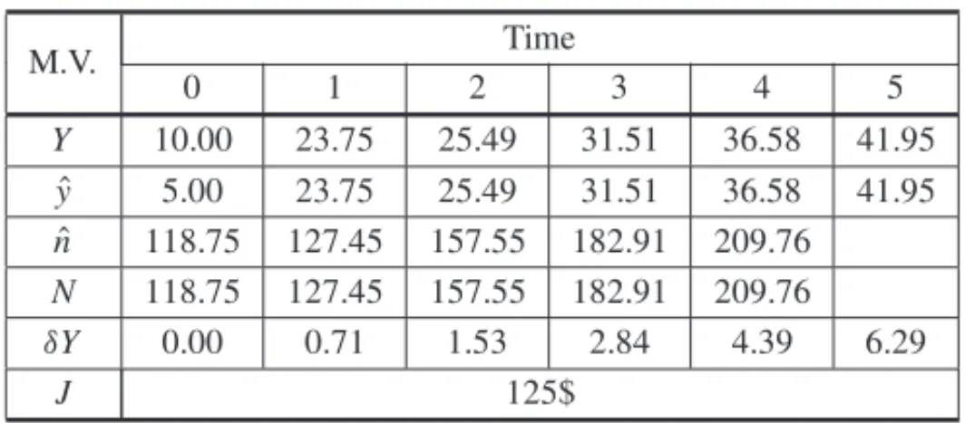
Table 2– Solution of the SQP model.
M.V. Time
0 1 2 3 4 5
Y 10.00 23.75 25.49 31.51 36.58 41.95 ˆ
y 5.00 23.75 25.49 31.51 36.58 41.95 ˆ
n 118.75 127.45 157.55 182.91 209.76 N 118.75 127.45 157.55 182.91 209.76 δY 0.00 0.71 1.53 2.84 4.39 6.29
J 125$
The following can be deduced from Table 2:
1. The inventory level and the production rate are both equal to its goal.
2. The total cost is 125$, which means that the quadratic programming model is better than the optimal control model.
3. The deterioration rate in the quadratic programming is less than in the optimal control model due to its reliance on the inventory levels.
4. The production rate is similar in two models at the end of the planning period.
3.3 Inventory level according to the two models
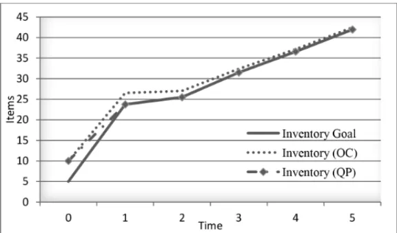
Figure 3– The inventory level, according to the optimal control and quadratic programming.
In the quadratic programming model, the convergence between inventory level and its goal is better than an optimal control model. This means the total cost of quadratic programming is less than the total cost of optimal control.
3.4 The effect of the stochastic demand on the results
This section presents the effect of the three cases of stochastic demand on the production rate and inventory level.
Figure 4 shows the demand rate becoming higher when the case of stochastic constraint is greater than or equal, (see Eq. 7), and vice versa.
Figure 5 shows the production rate become higher in the case of stochastic constraint is greater than or equal, due to the increase in the demand rate.
Figure 5– The production rate, according to the three cases of stochastic demand constraint.
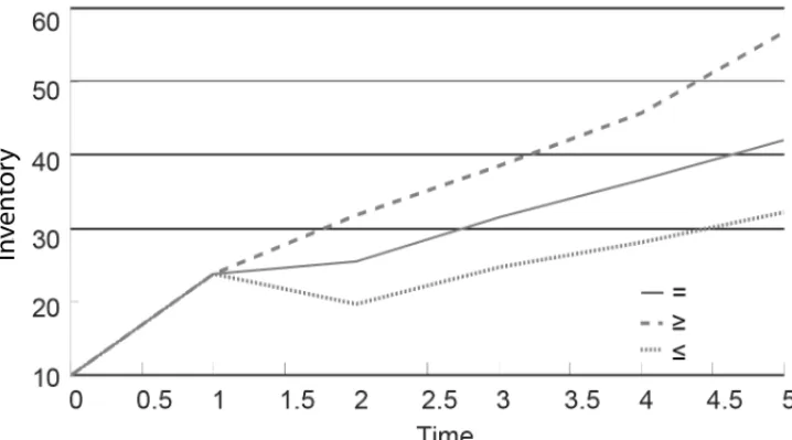
Figure 6 shows the inventory level becoming higher when stochastic constraint is greater than or equal, due to the production rate. The inventory levels at time (1) are similar in all cases, because the inventory, demand, and production at time (0) are similar in all cases (see Figs. 4, 5 and 6).
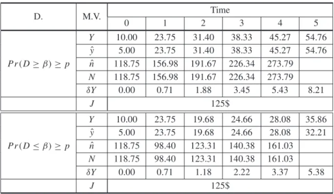
The total cost of three cases of demand is equal despite a difference in the production rates and inventory levels. This is due to realizing production goal rates and inventory goal levels in all of the cases.
Table 3– Solution of the SQP model with inequality stochastic demand constraint.
D. M.V. Time
0 1 2 3 4 5
Pr(D≥β)≥p
Y 10.00 23.75 31.40 38.33 45.27 54.76 ˆ
y 5.00 23.75 31.40 38.33 45.27 54.76 ˆ
n 118.75 156.98 191.67 226.34 273.79 N 118.75 156.98 191.67 226.34 273.79 δY 0.00 0.71 1.88 3.45 5.43 8.21
J 125$
Pr(D≤β)≥p
Y 10.00 23.75 19.68 24.66 28.08 35.86 ˆ
y 5.00 23.75 19.68 24.66 28.08 32.21 ˆ
n 118.75 98.40 123.31 140.38 161.03 N 118.75 98.40 123.31 140.38 161.03 δY 0.00 0.71 1.18 2.22 3.37 5.38
J 125$
4 CONCLUSION AND RECOMMENDATIONS
In this paper, two production-inventory system models; optimal control and SQP, were devel-oped. The models took into account stochastic demand, without shortage, and deteriorating items, to achieve the administration goals in the inventory level and hedge demand. Optimal conditions were derived for the optimal control model, along with an explicit solution to the production-inventory model under the periodic-review policy. Furthermore, a comparison between the op-timal control model and the SQP model results, in addition to a comparison between all three SQP models, were illustrated.
The SQP model was found to be better than the optimal control model when reaching optimality. At the end of the planning period, the production rate was found to be similar to the other two models. For the SQP model, production rate and inventory level were seen to increase in the case of the stochastic constraint, being greater than or equal. Total cost was controlled for all three SQP models, despite a difference in production rates and inventory levels. These models were found to be economically efficient for inventory control, with stochastic demand and deteriorat-ing items. This study could be extended to include the stochastic holddeteriorat-ing cost with and without shortage and inventory goal level as a function of demand.
ACKNOWLEDGEMENT
REFERENCES
[1] BANERJEES. 2011. Solution of Stochastic Inventory Models with Chance-Constraints by Intuition-istic Fuzzy Optimization Technique.International Journal of Business and Information Technology, 1(2): 137–150.
[2] BHOWMICKJ & SAMANTAGP. 2012. Optimal inventory policies for imperfect inventory with price dependent stochastic demand and partially backlogged shortages.Yugoslav Journal of Operations Research,22(2): 199–223.
[3] CASTELLANOD. 2015. Stochastic Reorder Point-Lot Size(r,Q)Inventory Model under Maximum Entropy Principle.Entropy,18(1): 1–18.
[4] CHOTAYAKULS & PUNYANGARMV. 2016. The Chance-Constrained Programming for the Lot-Sizing Problem with Stochastic Demand on Parallel Machines.International Journal of Modeling and Optimization,6(1): 56–60.
[5] DOGRUMK, REIMANMI & WANGQ. 2010. A stochastic programming based inventory policy for assemble-to-order systems with application to the W model.Operations research,58(4-part-1): 849–864.
[6] DOSTAL´ Z. 2009. Optimal quadratic programming algorithms: with applications to variational in-equalities Vol. 23. Springer Science & Business Media.
[7] FENGH, WUQ, MUTHURAMANK & DESHPANDEV. 2015. Replenishment Policies for Multi-Product Stochastic Inventory Systems with Correlated Demand and Joint-Replenishment Costs. Production and Operations Management,24(4): 647–664.
[8] GERMSR &VANFOREESTND. 2013. Optimal control of production-inventory systems with con-stant and compound poisson demand. University of Groningen, Faculty of Economics and Busisness. [9] HUM & YANGY. 2014. Modified echelon(r,Q)policies with guaranteed performance bounds for
stochastic serial inventory systems.Operations Research,62(4): 812–828.
[10] HURLEYG, JACKSONP, LEVIR, ROUNDYRO & SHMOYSDB. 2007. New policies for stochastic inventory control models – theoretical and computational results. Working paper, Cornell University, Ithaca, NY.
[11] KARKIR, BILLINTONR & VERMAAK. (Eds.). 2014. Reliability Modeling and Analysis of Smart Power Systems. Springer.
[12] KAZEMIZANJANIM, NOURELFATHM & AIT-KADID. 2010. A multi-stage stochastic program-ming approach for production planning with uncertainty in the quality of raw materials and demand. International Journal of Production Research,48(16): 4701–4723.
[13] KIESMULLER¨ GP. 2003. Optimal control of a one product recovery system with lead times. Interna-tional Journal of Production Economics,81-82(1): 333–340.
[14] KIMJS & JEONGWC. 2012. A Coordination Model Under an Order-Up-To Policy.Informatica, 23(2): 225–246.
[15] KLEYWEGTAJ, NORIVS & SAVELSBERGHMW. 2004. Dynamic programming approximations for a stochastic inventory routing problem.Transportation Science,38(1): 42–70.
[16] KUMARM, CHAUHANA & KUMARP. 2011. Economic production lot size model with stochastic demand and shortage partial backlogging rate under imperfect quality items.International Journal of Advanced Science and Technology (IJAST),31(1): 1–22.
[18] LEVI R, P ´ALM, ROUNDYRO & SHMOYSDB. 2007. Approximation algorithms for stochastic inventory control models.Mathematics of Operations Research,32(2): 284–302.
[19] MUBIRUK. 2014. Optimal Ordering Policies for Inventory Problems in Supermarkets under Stochas-tic Demand: A Case Study of Milk Powder Product.Proceedings of the 2014 International Confer-ence on Industrial Engineering and Operations Management, Bali, Indonesia: 245–253.
[20] MUBIRUK. 2015. Optimal Replenishment Policies for Two-Echelon Inventory Problems with Sta-tionary Price and Stochastic Demand.International Journal of Innovation and Scientific Research, 13(1): 98–106.
[21] OUARETS, KENNE´ JP & GHARBI, A. 2011. Hierarchical control of production with stochastic demand in manufacturing systems.AMO – Advanced Modeling and Optimization,13(3): 419–443. [22] PANX & LI, S. 2015. Optimal control of a stochastic production – inventory system under
dete-riorating items and environmental constraints.International Journal of Production Research,53(2): 607–628.
[23] PREKOPA´ A. 2013. Stochastic programming. Vol. 324. Springer Science & Business Media. [24] RAUPPF, DEANGELIK, ALZAMORAG & MACULANN. 2015. Mrp optimization model for a
production system with remanufacturing.Pesquisa Operacional,35(2): 311–328.
[25] REIMAN MI & WANGQ. 2015. Asymptotically optimal inventory control for assemble-to-order systems with identical lead times.Operations Research,63(3): 716–732.
[26] ROSSIR, TARIMSA, HNICHB & PRESTWICHS. 2007. Replenishment planning for stochastic inventory systems with shortage cost. InInternational Conference on Integration of Artificial Intelli-gence (AI) and Operations Research (OR) Techniques in Constraint Programming. 229–243. [27] SETHISP & THOMPSONGL. 2000. Optimal Control Theory Application to Management Science
and Economics, 2nd ed. USA: Springer.
[28] SHAPIROA & DENTCHEVAD. 2014. Lectures on stochastic programming: modeling and theory. Vol. 16. SIAM.
[29] SILVAFILHOOS. 2014. Optimal Aggregate Production Plans via a Constrained LQG Model. Engi-neering,6(12): 773–788.
[30] SOYSALMA. 2016. Research on Non-Stationary Stochastic Demand Inventory Systems. Interna-tional Journal of Business and Social Science,7(3): 153–158.
[31] TARIMSA, MANANDHARS & WALSHT. 2006. Stochastic constraint programming: A scenario-based approach.Constraints,11(1): 53–80.
[32] WANKE P. 2010. The impact of different demand allocation rules on total stock levels.Pesquisa Operacional,30(1): 33–52.
[33] WIERSEMAUF. 2008. Brownian motion calculus. John Wiley & Sons.
[34] YIF, BAOJUNB & JIZHOUZ. 2013. The optimal control of production-inventory system. In25th Chinese Control and Decision Conference (CCDC). China, 4571–4576.
[35] YOU F & GROSSMANNIE. 2011. Stochastic inventory management for tactical process planning under uncertainties: MINLP models and algorithms.AIChE Journal,57(5): 1250–1277.