Licenciado
Control in Distribution Networks with
Demand Side Management
Dissertação para obtenção do Grau de Doutor em Engenharia Electrotécnica e de Computadores
Orientador:
Prof. Doutor Rui Alexandre Nunes Neves da
Silva, Professor Auxiliar, Faculdade de
Ciências e Tecnologias da Universidade Nova
de Lisboa
Júri:
Presidente: Prof. Doutor Jorge Joaquim Pamies Teixeira
Arguente(s): Prof. Doutora Teresa Maria de Gouveia Torres Feio Mendonça
Prof. Doutor João Francisco Alves Martins
Vogais: Prof. Doutor José Manuel Prista do Valle Cardoso Igreja
Prof. Doutor Miguel José Simões Barão
Control in Distribution Networks with Demand Side Management
Copyright © Filipe André Barata, Faculdade de Ciências e Tecnologia, Universidade Nova de Lisboa.
The Faculdade de Ciências e Tecnologia and the Universidade Nova de Lisboa have the perpetual right, without geographical limits, to archive and publish this dissertation either in print or digital form, or any other medium that is still to be invented, and distribute it through scientific repositories, admitting its copy and distribution for educational or research purposes, as well as for non-commercial purposes, as long as the author and the editor are credited for their work.
I wish to express my gratitude to my Supervisor Professor Rui Neves-Silva for the opportunity he gave me and for the confidence he deposited in me, accepting this project inspired by him. I also like to thank his support and understanding in the most difficult periods of this journey, and by all his collaboration and advices which guided me until this moment.
Similarly, I would like to reserve a special acknowledgment to Professor José Manuel Igreja, for his priceless academic, professional, personal guidance and encouragement.
For this work I would like also to thank my CAT committee member Dr. João Martins, for is time, interest, and helpful comments.
I wish to personally thank my colleagues and friends from ISEL: Carla Viveiros, José Ribeiro, Luís Encarnação, Nuno Domingues, Nuno Guedes, Pedro Fonte, Ricardo Luís e Rita Pereira. These are fantastic people that provide me priceless moments and with whom I have the privilege to share a considerable part of my days since I have started my academic life.
Finally, and most importantly, I am thankful for the emotional support of my family. To Manuel Abreu Rodrigues, a tremendous friend that recently passed away, all my gratitude for his contagious joy that had provided me and my family unforgettable moments. His unexpected passing left me emotionally wounded, but allowed me to rethink better about my life. He will be sorely missed. To my Mother and Grandmother; two super women, an example of strength and determination. Despite all the drawbacks life brought them, they rose up and continued.
The way in which electricity networks operate is going through a period of significant change. Renewable generation technologies are having a growing presence and increasing penetrations of generation that are being connected at distribution level. Unfortunately, a renewable energy source is most of the time intermittent and needs to be forecasted.
Current trends in Smart grids foresee the accommodation of a variety of distributed generation sources including intermittent renewable sources. It is also expected that smart grids will include demand management resources, widespread communications and control technologies required to use demand response are needed to help the maintenance in supply-demand balance in electricity systems. Consequently, smart household appliances with controllable loads will be likely a common presence in our homes. Thus, new control techniques are requested to manage the loads and achieve all the potential energy present in intermittent energy sources.
This thesis is focused on the development of a demand side management control method in a distributed network, aiming the creation of greater flexibility in demand and better ease the integration of renewable technologies. In particular, this work presents a novel multi-agent model-based predictive control method to manage distributed energy systems from the demand side, in presence of limited energy sources with fluctuating output and with energy storage in house-hold or car batteries. Specifically, here is presented a solution for thermal comfort which manages a limited shared energy resource via a demand side management perspective, using an integrated approach which also involves a power price auction and an appliance loads allocation scheme.
The control is applied individually to a set of Thermal Control Areas, demand units, where the objective is to minimize the energy usage and not exceed the limited and shared energy resource, while simultaneously indoor temperatures are maintained within a comfort frame. Thermal Control Areas are overall thermodynamically connected in the distributed environment and also coupled by energy related constraints. The energy split is performed based on a fixed sequential order established from a previous completed auction wherein the bids are made by each Thermal Control Area, acting as demand side management agents, based on the daily energy price. The developed solutions are explained with algorithms and are applied to different scenarios, being the results explanatory of the benefits of the proposed approaches.
A forma como as redes elétricas operam está a atravessar um período de transformação significativa. As tecnologias de geração renováveis possuem uma presença crescente e a penetração desta geração ao nível da distribuição está a aumentar. Infelizmente, uma fonte de energia renovável é na maioria do tempo intermitente e necessita de algum tipo de previsão e antecipação de comportamento.
As têndencia actuais redes elétricas inteligentes preveêm que estas irão acomodar de uma forma integrada, formas de armazenamento de energia e uma variedade de fontes de geração distribuídas incluindo fontes renováveis intermitentes. É também expectável que as redes inteligentes irão incluir sistemas de gestão da procura e a difusão da comunicações e tecnologias de controlo necessários para que a resposta à procura auxilie no equilíbrio entre oferta e demanda em sistemas de energia elétrica. Eletrodomésticos inteligentes serão provavelmente uma presença comum nos nossos lares.
Desta forma, são necessárias novas técnicas de controlo para gerir as cargas por forma a aproveitar todo o potencial energético existente em fontes de energia intermitentes.
Esta tese foca uma metodologia de controlo para gestão da procura em redes distribuídas, para criar maior flexibilidade do lado da procura e facilitar a integração de tecnologias renováveis. Em particular, o trabalho apresenta um novo método de controlo predictivo multi-agente para gestão sistemas de redes de energia distribuídas do lado da procura, quando na presença de recursos energéticos limitados e flutuantes, e com armazenamento de energia em baterias domésticas ou de veículos. Especificamente, é aqui apresentada uma solução para conforto térmico que gere um recurso energético limitado e partilhado numa perspetiva de gestão da procura, utilizando uma abordagem integrada que envolve um leilão de preço de energia e um esquema de alocação de cargas domésticas.
O controlo é aplicado individualmente a um conjunto de Áreas de Controlo Térmico, unidades de demanda (consumidores), onde o objetivo é minimizar a utilização de energia sem exceder o
benefícios da abordagem proposta.
Acknowledgements ... iii
Abstract ... v
Resumo ... vii
Table of Contents ... ix
List of Figures ... xiii
List of Tables ... xix
List of Acronyms and Abbreviations ... xxi
1
Introduction ... 1
1.1 Introduction ... 1
1.2 Background ... 2
1.3 Motivation ... 3
1.4 Research Questions ... 5
1.5 Aimed Contributions... 5
1.6 Outline ... 7
2
Literature Review and Model Based Predictive Control ... 11
2.1 Introduction ... 11
2.2 Demand Side Management for Distribution Networks... 13
2.3 Model Based Predictive Control ... 18
2.3.1 Linear Plant Model ... 22
2.3.2 Nonlinear Plant Model ... 28
2.3.3 Generalized Predictive Control ... 29
2.3.4 Stability and Feasibility ... 33
2.3.7 Distributed Model Predictive Control ... 39
2.4 Multi-Agents systems (MAS) ... 44
2.4.1 MAS architectures ... 45
3
Dynamical Models and Scenarios Description ... 51
3.1 Introduction ... 51
3.2 Scenarios overview ... 52
3.3 Demand side management approach ... 56
3.4 TCA Dynamical Models ... 57
4
MPC and PI control in thermal comfort systems ... 65
4.1 Introduction ... 65
4.2 System description ... 66
4.3 Results ... 74
4.3.1 PI versus MPC. ... 76
4.3.2 MPC with “comfort zone” ... 77
4.3.3 MPC with “comfort zone” and constrained available power ... 79
4.3.4 Conclusions ... 80
5
Thermal Comfort with Demand Side Management Using
Distributed MPC ... 81
5.1 Introduction ... 81
5.2 Implemented global scenario ... 82
5.3 MPC formalization ... 84
5.3.1 Algorithm I - Implemented sequential scheme ... 90
6
DMPC for Thermal House Comfort with Sequential Access
Auction ... 91
6.1 Introduction ... 91
6.3 Access order with variable hourly sequence ... 110
6.3.1 Algorithm II - Implemented sequential scheme with variable hourly sequence ... 111
6.3.2 Results ... 112
6.4 Conclusions ... 119
7
DMPC for Thermal House Comfort with Sliding Load ... 121
7.1 Introduction ... 121
7.2 Algorithm III – Implemented shifting and loads allocation scheme ... 123
7.3 Results ... 126
7.3.1 One house scenario ... 127
7.3.2 Distributed scenario ... 131
7.4 Conclusions ... 139
8
Conclusions and Future Work Directions ... 141
8.1 Conclusion and Summary of Achievements ... 141
8.2 Recommendations for Future Work Directions ... 143
Figure 2.1. Smart Grid Roadmap (Bsria, 2014) ... 12
Figure 2.2. Venn diagram with implemented technologies. ... 12
Figure 2.3. Basic block diagram of MPC ... 20
Figure 2.4. Conceptual picture of the moving horizon in predictive control (Boom & Stoorvogel, 2010). ... 21
Figure 2.5. Hard constraint representation (Adapted from Froisy, 1994). ... 25
Figure 2.6. Soft constraint representation (Adapted from Froisy, 1994). ... 25
Figure 2.7. GPC control structure. ... 31
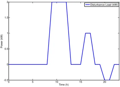
Figure 2.8. Disturbance load profile in the several prediction horizons. ... 34
Figure 2.9. Indoor temperature profile for the several prediction horizons. ... 34
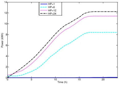
Figure 2.10. Power profile for the several prediction horizons. ... 34
Figure 2.11. Consumption profile for several prediction horizons. ... 35
Figure 2.12. Centralized MPC architecture (Scattolini, 2009). ... 36
Figure 2.13. Decentralized MPC architecture (Scattolini, 2009). ... 38
Figure 2.14. Distributed MPC architecture (Scattolini, 2009). ... 40
Figure 2.15. Single-agent control structure. (Adapted from Negenborn 2007). ... 46
Figure 2.16. Multi-agent single layer control structure. (Adapted from Negenborn 2007). ... 47
Figure 2.17. Multi-layer control structure. (Adapted from Negenborn 2007). ... 47
Figure 3.1. Typical smart grid architecture. ... 51
Figure 3.2. Typical energy distribution communication architecture for smart grids (Adapted from Siemens, 2014). ... 52
Figure 3.3. Implemented scheme. ... 53
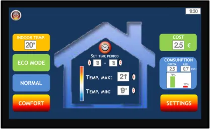
Figure 3.4. Thermal Control Area (TCA) smart thermostat controller vision. ... 54
Figure 3.5. Thermal Control Area concept... 54
Figure 3.6. Example of a TCA conceptual framework. ... 55
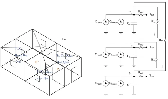
Figure 3.9. Generic schematic representation of thermal-electrical modular analogy for several
divisions (Barata et al., 2014b). ... 60
Figure 3.10. TCA divisions interaction simplified scheme; ... 62
Figure 3.11. Generalized house/TCA scheme example. ... 63
Figure 4.1. Block diagram of the implemented system. ... 67
Figure 4.2. MPC with constraints, system block diagram ... 72
Figure 4.3. Outdoor temperature. ... 75
Figure 4.4. Indoor temperature. ... 76
Figure 4.5. Power and energy consumption. ... 77
Figure 4.6. Temperature error with and without (MPC). ... 77
Figure 4.7. Case 1 - Indoor temperature with “comfort zone”. ... 78
Figure 4.8. Case 2 - Indoor temperature with “comfort zone”. ... 78
Figure 4.9. Power and energy consumption with “comfort zone”. ... 79
Figure 4.10. Indoor temperature evolution with limited power. ... 79
Figure 4.11. Power and energy consumption with limited power. ... 80
Figure 5.1. Implemented sequential architecture scheme. ... 83
Figure 5.2. Daily consumer profile. ... 86
Figure 5.3. Thermally coupled TCA’s. ... 86
Figure 6.1: Heat transfer between divisions example. ... 92
Figure 6.2: System implementation scheme block diagram. ... 93
Figure 6.3. Outdoor temperature forecasting ... 93
Figure 6.4. Scenario I - Disturbance forecasting and indoor temperature A1. ... 94
Figure 6.5. Scenario I - Disturbance forecasting and indoor temperature A2. ... 95
Figure 6.6. Scenario I - Disturbance forecasting and indoor temperature A3. ... 95
Figure 6.7. Scenario I - A1 power profile. ... 95
Figure 6.8. Scenario I - A2 power profile. ... 96
Figure 6.11. Scenario I - Power profile. ... 97
Figure 6.12. Scenario I - Heating/cooling total cost. ... 97
Figure 6.13. Scenario II - Disturbance forecasting and indoor temperature A1. ... 98
Figure 6.14. Scenario II - Disturbance forecasting and indoor temperature A2. ... 98
Figure 6.15. Scenario II - Disturbance forecasting and indoor temperature A3. ... 99
Figure 6.16. Scenario II –A1 power profile. ... 99
Figure 6.17. Scenario II –A2 power profile. ... 99
Figure 6.18. Scenario II –A3 power profile. ... 100
Figure 6.19. Scenario II -Global consumption characterization... 100
Figure 6.20. Scenario II -Power profile. ... 101
Figure 6.21. Scenario II -Heating/cooling total cost. ... 101
Figure 6.22. Scenario II -Batteries profile. ... 101
Figure 6.23. Scenario III - Disturbance forecasting and indoor temperature A1. ... 102
Figure 6.24. Scenario III - Disturbance forecasting and indoor temperature A2. ... 103
Figure 6.25. Scenario III - Disturbance forecasting and indoor temperature A3. ... 103
Figure 6.26. Scenario III –A1 power profile. ... 103
Figure 6.27. Scenario III –A2 power profile. ... 104
Figure 6.28. Scenario III –A3 power profile. ... 104
Figure 6.29. Scenario III - Global consumption characterization. ... 104
Figure 6.30. Scenario III - Power profile. ... 105
Figure 6.31. Scenario III - Heating/cooling total cost. ... 105
Figure 6.32. Scenario IV - Disturbance forecasting and indoor temperature A1. ... 106
Figure 6.33. Scenario IV - Disturbance forecasting and indoor temperature A2 ... 107
Figure 6.34. Scenario IV - Disturbance forecasting and indoor temperature A3 ... 107
Figure 6.35. Scenario IV –A1 power profile. ... 107
Figure 6.36. Scenario IV -A2 power profile... 108
Figure 6.39. Scenario IV - Power profile. ... 109
Figure 6.40. Scenario IV - Heating/cooling total cost. ... 109
Figure 6.41. Daily heating/cooling total cost. ... 110
Figure 6.42. Outdoor temperature forecasting (Toa). ... 113
Figure 6.43. Fixed consumption profile 𝐶𝑤11, and priority level of TCA1. ... 113
Figure 6.44. Fixed consumption profile 𝐶𝑤12, and priority level of TCA2. ... 113
Figure 6.45. Fixed consumption profile 𝐶𝑤13, and priority level of TCA3. ... 114
Figure 6.46. Implemented system. ... 114
Figure 6.47. Access order. ... 116
Figure 6.48. Disturbance forecasting and indoor temperature A1. ... 116
Figure 6.49. Disturbance forecasting and indoor temperature A2. ... 116
Figure 6.50. Disturbance forecasting and indoor temperature A3. ... 117
Figure 6.51. Consumption and constraints to heat/cool A1. ... 117
Figure 6.52. Consumption and constraints to heat/cool A2. ... 118
Figure 6.53. Consumption and constraints to heat/cool A3. ... 118
Figure 6.54. Global consumption. ... 118
Figure 6.55. Heating/cooling total cost. ... 119
Figure 7.1. Shifting load communication infrastructure. ... 122
Figure 7.2. Implemented shifting load scheme. ... 122
Figure 7.3. Total consumption characterization. ... 123
Figure 7.4. Implemented power distribution scheme starting in the Optimization Problem 1 (OPi) to OPNS. ... 124
Figure 7.5.Outdoor temperature forecasting (Toa). ... 127
Figure 7.6. Thermal disturbance forecasting. ... 127
Figure 7.7. Possible loads schedule combinations (PLSCs). ... 128
Figure 7.8. Total energy costs of FLSCS. ... 129
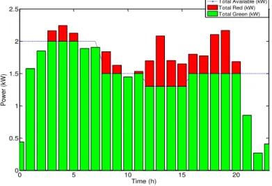
Figure 7.11. Used power to heat/cool the space and the maximum green resource available for
comfort. ... 131
Figure 7.12. Fixed consumption profile 𝐶𝑤11, and priority level of TCA1. ... 132
Figure 7.13. Fixed consumption profile 𝐶𝑤12, and priority level of TCA2. ... 133
Figure 7.14. Fixed consumption profile 𝐶𝑤13, and priority level of TCA3. ... 133
Figure 7.15. Access order. ... 133
Figure 7.16. Disturbance forecasting and indoor temperature A1. ... 134
Figure 7.17. Disturbance forecasting and indoor temperature A2. ... 134
Figure 7.18. Disturbance forecasting and indoor temperature A3. ... 135
Figure 7.19. Power profile A1. ... 135
Figure 7.20. Control input profile A1 ... 136
Figure 7.21. Power profile A2. ... 136
Figure 7.22. Control input profile A2. ... 137
Figure 7.23. Power profile A3. ... 137
Figure 7.24. Control input profile A3. ... 138
Figure 7.25. Batteries profile... 138
Table 2.1. Simulation parameters for the several prediction horizons ... 33
Table 2.2. Computational efforts under several prediction horizons ... 35
Table 4.1.Simulation parameters for PIvsMPC ... 76
Table 4.2. Simplified algorithm for MPC with “comfort zone”... 78
Table 6.1. Distributed parameters ... 94
Table 6.2. Scenario I - Penalty values ... 94
Table 6.3. Scenario III - Penalty values ... 102
Table 6.4. Scenario III - Cost comparisons ... 105
Table 6.5. Scenario IV - Penalty values ... 106
Table 6.6. Example of hourly access order sequence to green energy ... 111
Table 6.7. Bid value for each consumption level by agent. ... 114
Table 6.8. Scenario parameters. ... 115
Table 7.1.Scenario parameters ... 127
Table 7.2. Shifted loads characteristics ... 128
Table 7.3. Feasible Loads Sequence Combinations ... 129
Table 7.4. Distributed scenario parameters ... 131
Table 7.5. Bid value for each consumption level by TCA ... 132
Table 7.6. Shifted loads characteristics for distributed scenario ... 132
AMI Advanced Metering Infrastructure
ARMAX Autoregressive–Moving-Average Model with exogenous
inputs model
CPP Critical Peak Pricing
DER Distributed Energy Resources
DG Distributed Generation
DMS Distribution Management System
DR Demand Response
DMPC Distributed Model Predictive Control
DSM Demand Side Management
EMS Energy Management System
FLSC Feasible Loads Schedule Combinations
GPC Generalized Predictive Control
HVAC Heating Ventilation and Air Conditioning
I&C Interruptible and Curtailable Load
IL Interruptible Load
LQPC Linear-Quadratic predictive control
LTI Linear Time Invariant
MAS Multi Agent System
MBPC Model Based Predictive Control
MIMO Multiple-Input Multiple-Output
MO Market operator
MPC Model Predictive Control
MUSMAR Multistep Multivariable Adaptive Regulator
OCGT Open Cycle Gas Turbine
PLSC Possible Loads Schedule Combinations
PTR Peak Time Rebate
RES Renewable Energy Sources
RHC Receding Horizon Control
RTP Real Time Pricing
SGPC Stable Generalised Predictive Control
SISO Single-Input Single-Output
TCA Thermal Control Area
TCL Thermostatically Controlled Loads
TOU Time Of Use
Chapter 1
1
Introduction
1.1
Introduction
Traditional electric power systems consist of large power generating plants, interconnected via a high-voltage transmission lines, loading serving entities which deliver power to end users at lower voltages using local distribution networks.
Importance of distributed generators (DGs) has increased significantly over the past few years due to its potential for increasing reliability and lowering the cost of power through the use of on-site generation. Development of small modular generation technologies, such as photovoltaic, wind turbines and fuel cells has also contributed to this trend. However, novel operational and control concepts are needed to make a proper integration into the power grid system. Control strategies must be further developed to achieve the targeted benefits while avoiding negative effects on system reliability and safety. The current power distribution system was not designed to support distribution generation and storage devices at the distribution level; compatibility, reliability, power quality, system protection and many other issues must also be considered before the benefits of DGs can be fully obtained (Al-Hinai & Feliachi 2009).
A new emerging type of grid will soon be a reality. Smart Grids (SGs) are planned to include decentralized generation, active network management for generation and storage, where the actions of all connected agents to the electricity system can be intelligently integrated aiming for a sustainable, efficient and secure energy supply system. Future SGs are anticipated to support a variety of DG, including intermittent renewable sources (James & Jones, 2010).
electrical grid. Smart Grid is also positioned to take advantage of new technologies, such as hybrid plug-in electric vehicles (PEV), various forms of distributed generation, solar energy, smart metering, lighting management systems, distribution automation and many more.
In a scenario with strong presence of intermittent renewable energy sources (RES) that supply a set of houses, the new techniques must developed to deal with smart devices, energy management systems (EMS) such as programmable controllable thermostats and/or PEV charge, and be capable of making intelligent decisions based on smart prices and users comfort. Therefore, it is crucial to take into account a global solution that is able to take advantage of these features.
1.2
Background
Since the beginning of electricity grids, demand has fluctuated and supply has been provided to follow along. The intermittency of RES, such as wind or solar generation, stills nowadays the major challenge for the integration of these resources. The present trend in power systems is to connect more and more RES increasing significantly the security and the quality of supply. One of the most common solutions to mitigate the problem is operating energy sources, such as gas turbines or hydro power plants, balancing the variations. But, when the variations are significant and change rapidly, the backup source needs to be higher and faster, leading to increased carbon emissions. Also, widely used the frequency regulation is the direct measure of the balance between generation and system demand at any one instant, and must be maintained continuously within narrow statutory limits.
Another solution is the energy storage (Ribeiro et al. 2001; Koeppel & Korpas, 2006), if there is
decrease, reduction in the need for new power plants, transmission and distribution, reduction in air pollution and with a significantly increased in energy efficiency. With the growing interest in intermittent RES use, new opportunities and challenges are triggering and obliging these efforts to come true. Because of technology barriers and lack of automation, the traditional way of implementing DSM is via price incentives, i.e. by lowering tariffs at times when the aggregated demand is expected to be below average, so as to encourage the end user to shift flexible loads towards these periods (Saffre, 2010). But, with the new technologic advances and world trends around the SGs concept (Chebbo, 2007; Commission, 2006), and requiring this kind of grid intelligent control and management based on advanced communication, monitoring solutions, automation and metering, novel opportunities and challenges to DSM are emerging.
In the smart world, simple household appliances like dishwashers, clothes dryers, simple electric heaters or heating ventilation or air conditioning (HVAC) systems are planned to be fully controllable to achieve the network maximum efficiency. Renewable energy sources are expected to be a common presence and all kWh provided by these technologies should be efficiently applied. Active demand side management provide solutions to control the loads, adapting them to the current RES.
Being an actual theme, and despite the present trends and R&D efforts, SGs are still in the
“implementation phase”. More research is needed to provide solid solutions to overcome all the
constraints and turn into reality this ambitious vision. Smart Grids involve a mix of concepts: distributed generation, DSM, intelligent control, energy efficiency, intermittent RES, thermal comfort, load control and energy saving are some of them which are interconnected and should be integrated into solutions. Smart Grids are, therefore, the most efficient approach to integrate DG and RES in a coordinated way with demand management in a sustainable system (Blanquet et al., 2009). To take advantage from the innovative technology characteristics provided by
future smart grid, it is necessary the development of new models and control techniques which can support and manage all the mentioned concepts and, at the same time, deal with the network complexity and its distributed nature (Werbos, 2011).
1.3
Motivation
Currently buildings account for 40% of the world’s energy consumption and almost half of the
today’s greenhouse gas emissions. This means buildings contribute to more greenhouse gases
emissions than traffic; which is estimated at 31%. Industry is estimated at 28%. When we breakdown and analyse building’s energy consumptions, the most worrying aspect is that most
In Europe, the energy use in buildings has overall seen a rising trend over the past 20 years. For example, in 2009, households were responsible for 68% of the total final energy use in buildings, mainly due to space heating responsible for around 70% (Nolte, 2011). This increasing energy consumption is mainly to fulfil the demand for thermal comfort, being presently the HVAC systems the principal energy end use in buildings (Korolija et al., 2011). By these facts, it is socially, environmentally and economically imperative to decrease the energy consumption by increasing the buildings efficiency. A viable choice to achieve the reduction of energy consumption in the building sector is the application of demand response (DR) mechanisms. Demand Response program, is an efficient load management strategy for customer side, it is nowadays mostly used with the encouragement of customers to shift their habits wisely according to electricity price variation during daytime (Siano et al., 2014). The DR potential it is not sufficiently explored, being the two key challenges to work with diverse heterogeneous loads and with the distributed nature of renewable sources. New technology advances in communication are providing solutions to overcome the current electricity demand requirements. This new development has accelerated devising various industrial programs for scheduling utilization of residential appliances (Wang et al., 2015). This DR mechanisms combined with DSM methodologies will be relevant in the future distributed SGs (Mahmood et al., 2014), and provide solutions that allow buildings to be fully integrated and prepared to efficiently coexist in an dynamic and inconstant environment typically supported by renewable resources (Figueiredo et al, 2010). Nowadays the production of electricity system follows the load. However, the renewable sources of electricity are essentially intermittent and it is vital to provide flexibility to the grid to absorb the variations from these sources. In the intelligent energy system (Smart Grid) the production controls the consumption. For example, when the wind blows or the sun shines, buildings consumption must be automatically adjusted and consumers will go from being passive participants to be active players in the electricity system. Several solutions are emerging to deal with the variability, flexibility and poor controllability of the green sources and consequently on the ability to maintain the balance between demand and supply. Remark that, DSM strategies must have into account the control of many kinds of appliances, for instance, HVAC systems, lighting or electric vehicles charging.
1.4
Research Questions
With SGs, domestic customers will pass from static consumers into active participants in the production process. Final user’s participation can be achieved due to the development of new domestic appliances with controllable load. Shifting their electricity consumption in time or, by changing their work conditions, these devices can be controllable, adjusting the demand to the desired intermittent source without decreased the comfort of the residents. In distributed networks, aggregated to an intermittent source, an unlimited number of this kind of loads can exist, representing a control problem to achieve the network efficiencies, involving
stakeholder’s satisfaction. To incorporate this in system design and analysis, demand response
needs to be supported by scientific methodology based on analysis and models verifiable by experiment. How to improve energy efficiency using this domestic potential is still not well studied and needs to be a research topic.
Considering the mentioned above, this work aims providing solutions to answer the following research questions:
Q.1How, in a distributed network, can the demand be adjusted to an intermittent source to
maximize the energy efficiency?
Q.2How to improve energy efficiency using the domestic potential in a distributed network?
Q.3 Which control methods should be applied in a distributed network with demand side
management to obtain all the existing energy potential from intermittent energy sources?
The adopted work hypothesis to address the research question is defined below:
Using an integrated approach, that in a distributed environment, considers multi-agent
control scheme and an optimization MPC multi-objective approach with anticipative effect,
capable to deal in a DSM perspective, with fluctuating energy sources, smart load control,
thermal comfort and real-time price negotiation.
1.5
Aimed Contributions
Distributed Model Predictive Control (DMPC) to manage networks that is able to efficiently adapt the consumption to an intermittent renewable source. It provides news developments in DSM with renewable energy sources and backup fossil energy using an hourly auction mechanism access and a load allocation scheme that allows managing the loads in order to balance demand and supply. The proposed sequential multi-agent DMPC scheme for thermal house comfort and energy savings provides robustness, adjustment and flexibility to the global system. Also the work presents an energy usage optimization scheme with DSM in which the consumer as the flexibility to choose by the hour between comfort or energy savings.
The proposed integrated solution provides several scientific contributions that have been developed under the framework of this thesis:
C.1 New developments in DSM, for different thermal areas, exploit an integrated optimization approach able to cope with intermittent renewable energy sources and backup fossil energy using an hourly auction mechanism access - the obtained solution allows managing the loads in order to balance demand and supply. The DSM optimization process uses a routine that finds a constrained minimum of a quadratic cost function that penalizes the sum of several objectives, which based on energy forecasts and several other inputs, is able to adjust the energy consumption to an intermittent renewable resource or even restrict it to this type of resource in detriment of fossil sources. An auction mechanism allows stablishing an access order to the renewable source based on an hourly energy bid. Sequentially, the controllers transmit between them the information about the available energy;
C.2 TCA dynamic model with multi-zone dynamically coupled areas is developed - the developed model is built for infrastructures composed by several adjacent areas that may thermally interact among them. The dynamical model allows each room to be treated independently, with its own construction features, thermal disturbances, comfort requirements, energy costs and consumption needs. When distinct divisions thermally interact the information about the predicted indoor temperature is transmitted between them. This change of information allows to each controller a greater understanding about the surrounding environment and consequently improving the decision-making ability;
sequence is established and the energy price depends from the offered bid, amount and type (renewable or grid) of energy consumed;
C.4 Shifting load algorithm for loads allocation - customer sets features of flexible loads and the algorithm fits them in the most favourable time interval gap. Each customer select for each division, the characteristics of the loads, the load value, its
duration, the turned on time and the “sliding level” of the “shifted loads”. With this information the algorithm finds all the possible load combinations and from these selects only the feasible ones. The feasibility of the loads is related to the predicted hourly available power, so, at each instant the look forward and tries fitting the loads in gaps that privileges the consumption of renewable energy. Thus, in a distributed environment with energy and comfort constraints, the algorithm is able to find the best hour to turn on the loads;
C.5 Energy usage optimization scheme with DSM adjustable parameters - with the developed optimization scheme the consumer has the flexibility to choose hourly between comfort or energy savings. Each controller provides to the consumer a set of parameterizations which according to his consumption perspective, space occupancy schedule, indoor temperature preferences and energy cost, provides to the user the ability to be hourly in his most convenient state.
1.6
Outline
This dissertation is structured as follows:
Chapter 1– Introduction, here is performing a brief introduction with a background analysis,
followed by the research problem. The chapter also states the main original contributions of the work and in the end the outline of the thesis is presented.
Chapter 2–Literature Review and Model Based Predictive Control, the focus of this chapter
is to perform a background analysis on the main topics of the thesis, Demand Side Management, Multi-Agent-Systems and Model Based Predictive Control. The chapter also includes general review on distributed model predictive control formalization for complex large-scale dynamical systems.
Chapter 3 – Dynamic Models and Scenarios Description, the main ideas and models that
The elaboration of this chapter provided relevant matter that was originally included in part in the following publications (Barata et al., 2014a; Barata et al., 2014b).
Chapter 4–MPC and PI control in thermal comfort systems chapter presents the fundamental
approach towards the final developed structure. Is the first seed which allowed us to understand the problem, its dynamics and to verify that the MPC control strategy is suitable for the objective that is intended to be achieved. The methodologies are based on a predictive control structure associated to a PI controller and applied to the thermal house comfort in an environment with limited energy sources. The predictive control is compared with the traditional control methods used in thermal systems. Also, it was created a temperature “comfort zone” to weight only the temperatures outside the gap, instead of traditional system were all deviations are weight. Simulation results and analysis also complement two distinct situations where the system reacts differently if the indoor temperature is inside or outside the “comfort
zone”.
The elaboration of this chapter provided relevant matter that was originally included in part in the following publications (Barata et al., 2012a).
Chapter 5–Thermal Comfort with Demand Side Management Using Distributed MPC, this
chapter presents a DMPC methodology for indoor thermal comfort which simultaneously optimizes the consumption of a limited shared energy resource. Firstly, the global scenario and all the made assumptions that support the thesis are described. Also, the implemented sequential architecture scheme is pictured. Secondly, the control objective is defined and the tailored DMPC optimization problem is detailed, formalized and exemplified.
The Algorithm I which describe implemented sequential scheme is presented. This algorithm
represents the basic structure for more complex schemes.
Chapter 6–DMPC for Thermal House Comfort with Sequential Access Auction, this chapter
presents the obtained results achieved with the developed integrative methodology to manage energy networks from the demand side with strong presence of intermittent energy sources and with energy storage in house-hold or car batteries.
The results are pictured with and without batteries support and two different approaches are considered, the energy split based on a fixed sequential order, and with the energy split varying hourly based on a bid value directly related with the consumption profile behaviour. The
Algorithm II, which describes implemented sequential scheme with variable hourly sequence
and energy storage, is also presented.
Chapter 7–DMPC for Thermal House Comfort with Sliding Load chapter presents the
developed DMPC integrative solution which is able to, in a distributed network with multiple TCAs, adjust the demand to an intermittent limited energy source, using load shift and maintaining the indoor comfort. The Algorithm III which describes the implemented shifting
and loads allocation scheme is presented followed by the results and its analysis. The elaboration of this chapter provided relevant information that was included in the following publications (Barata et al., 2013c) and more detailed in (Barata et al., 2014c).
Chapter 8–Conclusions and Future Work Directions,in this last chapter, discusses the main
Chapter 2
2
Literature Review and Model Based
Predictive Control
2.1
Introduction
Future SGs are expected to include distributed generation, demand side management, intelligent control, energy efficiency, intermittent RES, thermal comfort, load control, real-time price negotiation and energy saving (IEA, 2011). These concepts are the smart grid bases, where the actions of all agents connected to the electricity system can be intelligently integrated aiming for a sustainable, efficient and secure energy supply system.
Being an actual theme, and despite the present trends and R&D efforts, SGs are now giving the firsts steps in the implementation phase, Figure 2.1, with small projects and grid prototypes all over the world (EcoGrid, 2014; DOE, 2014). More research is needed to offer solid solutions to overcome all the constraints and turn real this ambitious vision.
In a scenario with strong presence of intermittent RES that supply a set of houses, it is possible to manage several loads in each house in order to: 1) adjust the demand to the supply; 2) maintain indoor thermal comfort; 3) achieve lower energy costs 4) reduce CO2 emissions. Using
Figure 2.1. Smart Grid Roadmap (Bsria, 2014)
The method uses the match results between demand and supply to decide the control actions to be implemented on the demand side. It is considered environmental and pre-establish variables as a decision-making factor. By using this active DSM control, the optimal control strategies for various appliances can be generated whilst maximum utilisation of energy supplied from intermittent systems is guaranteed. In a distributed network, with several loads at different locations control actions applied for solving a local energy problem can create lack of energy at a different location in the network. Therefore, coordination control strategies are required to make sure that all available control actions serve the same objective. To support the idea, it is consider multi-agent control schemes in which each agent will employ a model-based predictive control approach. The agents communicate and negotiate in a distributed network environment, to improve decision making, and, by adjusting the demand to the source, the maximum energy potential existent in the intermittent source can be achieved.
Figure 2.2. Venn diagram with implemented technologies.
MBPC
At the same time, as referred, is also desirable no or negligible impact on end users/occupiers. Thus, this literature review intend to show what are the main research trends related with the three main support ideas that interact in this work, DSM, Multi-Agent Systems (MAS) and Model Based Predictive Control (MBPC), Figure 2.2.
2.2
Demand Side Management for Distribution Networks
To reach important reduction in CO2 emissions, the RES will be the main contributors to the
electricity generation systems. Presently, the solar and wind power, are the renewable energy technologies that are commercially available with sufficient scalable. Although the expected growth of these sources through to 2020 target is envisioned, there are real concerns about the variability, flexibility and poor controllability of the sources and consequently on the ability to maintain the balance between demand and supply. The growing uncertainty in power systems coupled with the introduction of power markets calls for the development of new tools for planning, operations and market-based decision-making. To deal with this uncertainty due to the dissemination of renewables, the systems will need, for example, to apply bigger amounts of reserve that is generally provided by a combination of synchronised and standing reserve. Besides to synchronise reserve provided by part-loaded plant, the balancing task will also be supported by standing reserve, which is supplied by a plant with higher fuel and environmental costs, such as Open Cycle Gas Turbine (OCGT), or through more desirable techniques such as storage facilities or DSM.
Energy efficiency, the user decreases the demand for energy without sacrificing the benefits received from energy (e.g. installing building insulation, purchasing more efficient appliances);
Conservation, the consumer decreases his energy demand by reducing their energy usage (e.g. adequate thermostat temperatures, turning off lights);
Load management, the energy demand is reduced during periods of peak demand when capacity is limited and the cost of energy provision is high;
Public information, which encourages customer participation in energy efficiency, conservation, and/or load management activities through public campaigns, direct to customer communication, or increasing customer access to information about their consumption of energy services.
DSM directly benefits utilities in the following ways:
Distribution - only utilities avoid having to purchase additional peaking and base-load energy resources. From the volatile wholesale energy market;
Electricity generating utilities avoid the cost of securing fuel and pollution abatement for peaking and base-load power plants, while deferring expensive investments in new power plants and their associated compliance costs;
Both kinds of utilities avoid costly investments in new transmission and distribution infrastructure.
Utilities may in turn pass these savings on to consumers, resulting in lower utility bills. In addition, DSM directly benefits utility customers in the following ways:
Many DSM programs provide financial incentives (such as rebates, bill credits, lower rates, or low interest financing) to encourage customers to make choices that reduce their energy consumption overall or during periods of peak demand;
By encouraging customers to reduce their energy usage or to consume energy during times when energy services are less costly, DSM programs help customers to reduce their monthly utility bill.
Demand response is a class of DSM programs in which electricity companies offer incentives to clients to reduce their demand for electricity during periods of critical system conditions or periods of high market power costs. DR programs are normally classified according to the
customer motivation method and the criteria with which load reduction “events” are triggered or
initiated. So, when the utility offers customers payments for reduction of demand during specified periods, the program is called load response. But, when customers voluntarily reduce
their demand in response to forward market prices, the program is called price response.
generate or buy the energy. In this context, brief descriptions of these DR techniques that are presently worldwide being applied and studied are now described.
Load-Response Programs
In load-response programs, utilities offer customers payments for reducing their electricity demand for specified periods of time.
Direct load control
Direct load control is applied to domestic appliances that can be switched on and off during periods of time using remote appliance controllers. The most common applications are the ones that account for the most significant portion of energy demand, HVAC systems and water heaters;
Load limiters
Load limiters have the intent to limit the power that can be used by consumers. This approach temporarily disconnects parts of the installation, most often the HVAC or electrical heating during power peaks. This scheme can also provide some flexibility to users to decide which appliances to use now and what can be delayed;
Interruptible and Curtailable Load (I&C)
Interruptible and Curtailable-load programs are relatively simple to implement, the customers agree to decrease or turn off pre-established loads for a period of time when notified by the utility. Clients can switch off loads or adjust settings. Utilities must notify customers before an interruptible/curtailable load event. As reward, participants receive lower electricity bills during normal operation, as well as additional incentives for each event;
Frequency regulation
System frequency is the direct measure of the balance between generation and system demand at any one instant and must be maintained continuously within narrow statutory limits. Recently, there have been initiatives to investigate a technology that can be incorporated into electrical appliances to provide frequency regulation (Dynamic Demand, 2014);
Scheduled Load
Price-Response Programs
These programs allow customers to voluntarily reduce their demand in response to economic signals.
Time of use pricing
Time of use (TOU) tariffs are designed to more closely reflect the production and investment cost structure, where rates are higher during peak periods and lower during off-peak periods. Basically, instead of a single flat tariff for energy use, TOU tariffs are plan to be higher when electric demand is higher, meaning that when you use energy is as important as how much you use. These programmes are commonly practiced in a large number of countries, particularly for households with electric heating;
Dynamic/Real Time Pricing (RTP)
The dynamic imposed by the existing deregulated market is based on real time system of supply and demand. Prices change time to time and hour to hour depending upon these two factors. By exposing customers to RTP i.e. time-varying prices, they can have a better view of the prevailing market and the information and incentive to reduce their demand at peak times or critical peak prices (CPP) and by this way provide a financial incentive for participants to shift optional activities, such as clothes washing and drying and dishwashing, to times other than critical peak periods;
Demand bidding
Demand bidding programmes are available when the customer is willing to negotiate is consumption needs in detriment of cost reductions. So, the client is disposed to decrease or sacrifice his consumption of electricity at a certain predetermined price. For example, this
technology can be applied to a smart thermostat which controls the indoor comfort equipment’s. So, depending from real time electricity price levels, the thermostat can be programed to allow different sceneries in different schedules.
In buildings, novel solutions that integrate occupant behaviour within the building in relation to energy consumption are emerging (Virote & Neves-Silva, 2012).
As showed, DSM will have an important role in the future smart grids architecture (Chen et al.,
2010; Luo et al., 2010) and by this reason many studies are being performed involving the mentioned DSM techniques to provide future implementation solutions.
Callaway (2009), with the goal of delivering services such as regulation and load following, developed new methods to model and control the aggregated power demand from a population of thermostatically controlled loads (TCLs). The researcher manipulates the temperature set point in order to control the demand curve and adapt it to a wind plant power source. The work showed that it is possible the demand to follow the source with small changes in the nominal thermostat temperature set point. With similar objective, Jun (2009), developed an algorithm capable of controlling loads based on the available supply at certain time. The objective of the algorithm is to minimize the impact on users and at the same time maximize the match between demand and supply through identifying the best combinations of different demand side control options such as load shifting, load control (on/off control and proportional control) and load recover for various demand loads.
A potential application for controllable domestic heat loads, and flexible distributed generation in power systems with significant capacities of uncertain wind generation is described in (Savage et al, 2008). Heat load is effectively controlled by remote adjustment of thermostat set points. The system transmit a signal to reduce heating load set points when net demand is greater than the forecast value and a reserve shortfall was imminent. Zaidi et al., (2010) follows a DSM approach, where unessential loads get selectively disconnected from the grid in an under-generation scenario. In order to automatically detect unessential loads, load recognition on the basis of measured consumption data can be performed. With the same objective of peak shaving and balance between demand and supply, (Molderink et al., 2010), shows that with the use of good predictions, in advance planning and real-time control of domestic appliances, better matching of demand and supply can be achieved. With a similar approach, several other studies can be found (James & Jones, 2010; Krishnappa, 2008).
As presented, several methods are focus in the development of load control manipulation models, however, DSM is also been studied via models that use electricity incentive prices to promote load management (Yang et al., 2006; Hamidi et al., 2008; Aalami et al., 2008; Yu & Yu 2006; Shaikh & Dharme, 2009).
costs. New models and control techniques must be developed to be capable of not only to manage loads based on the available supply at a certain time, but also by negotiating in real time the energy price and the consumer comfort (without significantly compromising the user satisfaction) in order to guarantee the balance between demand and the intermittent source. In a scenario with strong presence of intermittent RES that supply a set of houses, the new solution must include smart devices, energy management systems (EMS) such as programmable controllable thermostats and/or PEV charge, capable of making intelligent decisions based on smart prices and users comfort.
2.3
Model Based Predictive Control
The firsts predictive controllers concepts were born from optimal control methodologies, such as the Linear Quadratic (LQ) or the Linear Quadratic Gaussian (LQG) controllers in the
early’70s (Anderson and Moore, 1971). Only in late 70's that the first two truly MPC control laws arise, the Identification-command (IDCOM) and the Dynamic Matrix Control (DMC), which are acknowledged as the roots of MPC. These two methods share some common features which established the basis of MPC.
The predictive control based on model MBPC is nowadays as one of the most popular and efficient control strategies in industry. So, during the last two decades a growing interest has been granted to model predictive control (MPC) due to its ability to handle constraints in an optimal control environment (Moroşan et al., 2010; Mosca, 1995). It is expected that soon MPC may substitute the majority of the classic controllers that are becoming inefficient in complex environments.
MPC is a form of control in which the current control action is obtained by solving on-line, at each sampling instant, a finite horizon open-loop optimal control problem, using the current state of the plant as the initial state, the optimization yields an optimal control sequence and the first control in this sequence is applied to the plant. The major advantages that have contributed for the success of this method are (Orukpe 2005; Jimenez 2000):
It handles multivariable control problems naturally, Single-Input/Single-Output SISO) and Multiple-input/Multiple-Output (MIMO) formulations are similar;
Difficult dynamics such as dead-times, unstable or non-minimum phase systems can be easily handled;
It can take account of actuator limitations The incorporation of constraints in the manipulated and controlled variables and/or states is a simple task. Constraints can be considered at the controller design stage and the resulting optimisation problem can often be solved using standard Linear Programming (LP) or Quadratic Programming (QP) tools. It also allows operation closer to constraints, hence increased profit;
MPC controllers have been developed either for linear or non-linear models;
Methods which guarantee the stability of the closed-loop system are available;
Robustness features can be enhanced through tuning parameters or optimisation methods. Constraint handling is, indeed, one of the most appealing properties of MPC, since limits of several kinds always occur in practice.
Constraints can be used to describe several security limits, physical restrictions, technological requirements and so on. These requirements must be handled at the controller design stage to avoid undesirable performance. Constraints have two main objectives. They can be used to increase the accuracy of the model, incorporating on it the actuator and plant limits and also be used as tuning knobs to describe control requirements or specifications. Typically, optimal operating point lies close to (or on) one or several limits and therefore, representing an advantage from an economical point of view when it operate as close to the constraint boundary as possible. Constraints can be classified according to different criteria. The following classification of constraints, according to practical considerations, is due to Álvarez and de Prada (1997):
Physical constraints. These limits, which must never be surpassed, are determined by the physical limitations of the system;
Operating constraints. These bounds are fixed by the plant operators to specify the optimal operating region. The operation constraints are more restrictive than he physical limits;
Optimization or set point conditioning constraints. These limits, more restrictive than the operating constraints, are used only if the set point conditioning technique is applied;
Working constraints. These are the actual constraints considered by the controller to determine the feasible region. The working constraints are obtained by choosing the most restrictive among the physical, the operating and the optimization limits. Apart from constraint handling, the relevant issues of stability and robustness have been successfully tackled in the last decade.
Reference Trajectory - represents the desire signal to future outputs. The previous knowledge of this trajectory provides the anticipative effect of this controller;
Model - the mathematical model, linear or nonlinear, that represents the process must be capable to describe its dynamic behavior with sufficient accuracy;
Predictor- trough the mathematical model provides the future outputs based on the actual plant information;
Optimizer- minimizes the cost function at every time sample to obtain the control action that guaranties the system performance. When linear models are used and the problem is unconstraint, the quadratic cost function presents a analytical solution, otherwise, some numeric optimization methods must be used.
As can be seen, the presence of the plant model is a necessary condition for the development of the predictive control. The success of MPC depends on the degree of accuracy of the plant model (Zheng 2010).
Figure 2.3. Basic block diagram of MPC
Predictive control uses the receding horizon principle. This means that after computation of the optimal control sequence, only the first control sample will be implemented, subsequently the horizon is shifted one sample and the optimization is restarted with new information of the measurements. The prediction horizon remains the same length despite the repetition of the optimization at future instants. Since the state prediction x and hence the optimal sequence u* depend on the current state measurements 𝑥(𝑘), this procedure introduces feedback into the MPC law, providing a degree of robustness to modelling errors and uncertainty. Figure 2.4 explains the idea of receding horizon.
OPTMIZER
MODEL
(ESTIMATOR)
PROCESS
PREDICTOR
control Predicted
error
Predicted output
output
+
–
REFERENCE
TRAJECTORY
COST
FUNCTION CONSTRAINTS
u(k)
𝑦 (𝑘 + 1) r(k)
y(k)
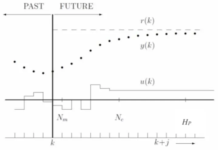
Figure 2.4. Conceptual picture of the moving horizon in predictive control (Boom & Stoorvogel, 2010).
In Figure 2.4 Nm, NC and HP represents is the minimum cost horizon, the control horizon and
prediction horizon respectively. At time k the future control sequence {𝑢(𝑘|𝑘), . . . , 𝑢(𝑘 + 𝑁𝑐 −
1|𝑘)} is optimized such that the performance-index J(u, k) is minimized subject to constraints.
At time k the first element of the optimal sequence (𝑢(𝑘) = 𝑢(𝑘|𝑘)) is applied to the real
process. At the next time instant the horizon is shifted and a new optimization at time k+1 is
solved.
The goal of MPC is to minimize a cost function over a given prediction horizon period. This cost function should give an indication for the performance of the system. The control signal contains the setting for the control measures that are able to influence the system, and the constraints may contain the upper and lower bounds on the control signal, but also linear or non-linear equality and inequality constraints on the control inputs and the states of the system. In MPC, control decisions, system inputs, u(k) are made at discrete time instants k = 0,1,2,...,
which usually represent equally spaced time intervals. At decision instant k, the controller
samples the state of the system x(k) and then solves an linear optimization problem of the
following form to find the control action:
𝑚𝑖𝑛𝑢 𝐽(𝑥, 𝑢; 𝑥(𝑘)), (2.1)
𝑠. 𝑡. 𝑥(𝑘 + 1) = 𝐴𝑥(𝑘) + 𝐵𝑢(𝑘), (2.2)
𝑢 ∈ 𝒰,
where x(k) ℝn and u(k) ℝm, and A ℝn×n, B ℝn×m, are known matrices with constant
entries of corresponding entries. The cost function J(k) is linear quadratic, Linear Quadratic
Predictive Control (LQPC), with symmetric weighting matrices Q and R, where Q ≥ 0, R > 0,
and 𝒰 is an admissible control set.
𝑚𝑖𝑛
𝑢0,…,𝑢𝐻𝑃−1= ∑ 𝑥(𝑘)
𝑇𝑄𝑥(𝑘) + 𝑢(𝑘)𝑇𝑅𝑢(𝑘) 𝐻𝑃−1
𝑘=0
, (2.3)
𝑠. 𝑡. 𝑥(𝑘 + 1) = 𝐴𝑥(𝑘) + 𝐵𝑢(𝑘), 𝑘 = 0, … 𝐻𝑃− 1, (2.4)
𝑢(𝑘) ∈ 𝒰, 𝑥(𝑘 + 1) ∈ 𝒳, 𝑘 = 0, … , 𝐻𝑃− 1,
𝑥0= 𝑥(𝑡) ≡ 𝑥(𝑘).
The future states are described as,
𝑋̂(k) = 𝐺𝛥𝑈(𝑘) + 𝛤𝑥(𝑘), (2.5)
𝑋̂(𝑘) = [𝑥 (𝑘 + 1)⋮ 𝑥 (𝑘 + 𝐻𝑃)
] = [𝐴⋮ 𝐴𝐻𝑃
] ⏟
𝛤
𝑥(𝑘) + [𝐵⋮ ⋯ 0⋱ ⋮ 𝐴𝐻𝑃−1𝐵 ⋯ 𝐵
] ⏟
𝐺
[𝛥𝑢(𝑘)⋮
𝛥𝑢(𝑘 + 𝐻𝑃− 1)
] ⏟
𝛥𝑈
,
(2.6)
𝑋̂0= 𝛤𝑥 (𝑘). (2.7)
For regulation proposes, and considering the general case which intent to lead the state to zero, the linear MPC without constraints solution of (2.3) is given by:
𝛥𝑈∗= −𝐾
𝑐𝑥 (𝑘) = −(𝐺𝑇𝑄𝐺 + 𝑅)−1𝐺𝑇𝑄𝑋̂0 (2.8)
and implementing the first element of the optimal prediction at each sampling instant k defines a
receding horizon control law
𝑢(𝑘) = 𝛥𝑈∗(1).
(2.9) Remark that if 𝒰 and 𝒳 are polyhedral (a finite intersection of half-space), this is a Quadratic Program, that can be can be solve fast, efficiently and reliably, using modern solver tools.
2.3.1
Linear Plant Model
For linear systems, the dependence of predictions x(k) on u(k) is linear. A quadratic
minimization cost function as (2.3) is therefore a quadratic function of the input sequence vector
u. Thus J(k) can be expressed as a function of u in the form,
𝐽(𝑘) = 𝒖𝑇(𝑘)𝐻𝒖(𝑘) + 2𝑓𝑇𝒖(𝑘) + 𝑔, (2.10)
where H is a constant positive definite (or possibly positive semi-definite) matrix, and f, g are
respectively a vector and scalar which depend on x(k). The online MPC optimization therefore
𝑚𝑖𝑛
𝑢 𝒖
𝑇(𝑘)𝐻𝒖(𝑘) + 2𝑓𝑇𝒖(𝑘).
(2.11) In the absence of constraints, unconstrained MPC, the optimization u*(k) = 𝑚𝑖𝑛
𝐮 𝐽(𝑘) has a
closed-form solution which can be derived by considering the gradient of J with respect to u:
𝛻𝑢𝐽 = 2𝐻𝒖 + 2𝐹𝑥(𝑘). (2.12)
Clearly 𝛻u𝐽 = 0 must be satisfied at a minimum point of J, and since H is positive definite (or
positive semidefinite), any u such that 𝛻u𝐽 = 0 is necessarily a minimum point. Therefore the
optimal u* is unique only if H is non-singular and is then given by,
𝒖∗(𝑘) = −𝐻−1𝐹𝑥(𝑘). (2.13)
Remark that, sufficient conditions for H to be non-singular are for example that R > 0 or Q, 𝑄̅ >
0 and the pair (A,B) is controllable.
If H is singular (i.e. positive semi-definite rather than positive definite), then the optimal u* is non-unique, and a particular solution of 𝛻u𝐽 = 0 has to be defined as,
𝑢(𝑘) = −𝐻†𝐹𝑥(𝑘), (2.14)
where H† is a left inverse of H (so that H†H = I).
Implementing the first element of the optimal prediction u*(k) at each sampling instant k defines
a receding horizon control law. Since H and F are constant, this is a linear time-invariant
feedback controller u(k) = KC x(k), where the gain matrix KC is the first row of −H−1F for the
single-input case (or the first nu rows for the case that u has dimension nu), i.e.
𝑢(𝑘) = 𝑢∗(𝑘|𝑘) = 𝐾
𝐶𝑥(𝑘), (2.15)
𝐾𝐶 = −[𝐼𝑛𝑢 0 … 0]𝐻−1𝐹. (2.16)
Constrained MPC is used when structural limitations of the system to be controlled usually leads to control restrictions and avoiding such limitations may cause harmful effects as unstable cycle. However, for performance purpose, the control system should try to use the system as close to those limits as possible, without crossing them. Therefore, MPC uses a more direct approach by finding the optimal control in such a way that constraints are not violated.
Most typically, linear input and state constraints likewise imply linear constraints on u(k) which
can be expressed