Adversarial machine learning: denial of services recognition

(1)

F

ACULDADE DE

E

NGENHARIA DA

U

NIVERSIDADE DO

P

ORTO

Adversarial Machine Learning on

Denial of Service Recognition

Nuno Jorge Dias Carneiro Martins

M

ASTER

’

S

D

ISSERTATION

Mestrado Integrado em Engenharia Informática e Computação Supervisor: José Magalhães Cruz

Co-Supervisor: Pedro Henriques Abreu

(2)

(3)

Adversarial Machine Learning on

Denial of Service Recognition

Nuno Jorge Dias Carneiro Martins

Mestrado Integrado em Engenharia Informática e Computação

(4)

(5)

Abstract

Online services have seen a rise on popularity over the last two decades. Social networks, banking applications, blogs and many other services are increasingly being embedded in the daily lives of every citizen, but many of them are targeted by intruders with malicious intent. Attackers often disrupt these services, or use them to obtain personal information, send spam or spread malware, using a high variety of techniques.

Cybersecurity is the area that studies protection against cyber-attacks, offering many defen-sive measures. With the growing pace at which new attacks are created, conventional detection methodologies based on anomaly detection or attack knowledge are often not enough, and machine learning is adopted.

The usage of machine learning has grown in recent years, mainly due to advances in computing power, and has successfully been applied to a high variety of areas, such as intrusion detection. Although the machine learning classifiers can successfully identify attacks in many cases, they are often themselves a target, by attackers that create specific samples that aim to deceive the classifiers, which are called "adversarial examples".

Adversarial machine learning is an area of study that examines both the generation and de-tection of adversarial examples, and has been extensively researched specifically in the area of image recognition, where small modifications are performed on images that cause a classifier to be deceived.

The goal of this dissertation was to perform an analysis on the behaviour of adversarial ma-chine learning techniques on Denial of Service attacks, where an attacker aims to disrupt an online service to its intended users by flooding it with seemingly valid requests. To achieve this goal, we first studied different adversarial attack and defense strategies which were initially applied to im-age recognition, and explored their applications to Denial of Service attack contexts, by analyzing multiple works on adversarial malware and intrusion detection, which are the most similar applica-tion scenarios in literature. To the best of the authors knowledge, no adversarial defense strategies were ever explored for these scenarios.

We then proposed multiple experiments on two Denial of Service datasets, where we initially trained multiple state of the art classifiers on the original datasets, and then inserted perturbations on the datasets using four adversarial attack strategies. The results showed that there was a sig-nificant deterioration on the performance of all classifiers on both datasets, with the Denoising Autoencoder being the most resilient classifier for attacks with larger pertubations. We then tested four different adversarial defense strategies, and all strategies showed an improvement in resisting adversarial examples compared to the baseline classifiers against adversarial attacks, with defense strategies that revolve around including adversarial examples in the training set being the most effective ones.

(6)

(7)

Resumo

Serviços online têm visto um aumento na popularidade nas últimas duas décadas. Redes sociais, aplicações bancárias, blogs e muitos outros serviços estão cada vez mais presentes no quotidiano de cada cidadão, mas muitos deles são alvos de intrusos com intenções maliciosas. Os atacantes geralmente interrompem esses serviços ou utilizam-nos para obter informações pessoais, enviar spam ou espalhar malware, usando uma grande variedade de técnicas.

Cibersegurança é uma área que estuda proteção contra ciberataques, oferecendo diversas me-didas defensivas. Com o crescente ritmo com que novos ataques são criados, métodos conven-cionais de deteção baseadas em deteção de anomalias ou conhecimento prévio dos ataques são muitas vezes insuficientes, sendo machine learning usado.

A utilização de machine learning tem aumentado nos últimos anos, principalmente devido aos avanços no poder computacional de dispositivos, e tem sido aplicado com sucesso numa grande variedade de áreas, como detecção de intrusões. Embora os classificadores machine learning possam identificar com sucesso os ataques em muitos casos, eles também podem ser um alvo por invasores que criam amostras específicas cujo objetivo é enganar os classificadores, que são chamados de amostras adversárias.

Adversarial machine learning é uma área de estudo que examina tanto a geração como a de-tecção de amostras adversárias, e tem sido vastamente pesquisada na área de reconhecimento de imagem, onde pequenas alterações são realizadas em imagens que fazem com que um classificador realize previsões incorretas.

O objetivo principal desta dissertação foi realizar uma análise do comportamento de diferentes técnicas de adversarial machine learning em ataques de negação de serviço, onde um atacante tenta afetar a disponibilidade de um serviço online, ao inundá-lo com pedidos aparentemente váli-dos. Para alcançar este objetivo, começamos por estudar diferentes estratégias de ataque e defesa com adversários que foram inicialmente aplicadas a reconhecimento de imagem, e exploramos as suas aplicaçoes a ataques de negação de serviço ao analisar multiplos trabalhos sobre deteção de intrusões e malware com adversários, já que é o cenário de aplicação mais semelhante na literatura existente. Pelo conhecimento dos autores, a aplicação de defesas adversárias nunca foi explorada nestes contextos.

Assim, nós propusemos múltiplas experiências a realizar em dois datasets de negação de serviço, onde inicialmente treinamos multiplos classificadores estado da arte nos datasets origi-nais, e depois inserímos perturbações nos datasets usando quatro estratégias de ataque adversário. Os resultados mostraram que houve uma perda significativa no desempenho de todos os classifi-cadores em ambos os datasets, com o Denoising Autoencoder sendo o classificador mais resistente contra ataques com maiores perturbaçoes. De seguida testamos quatro estratégias de defesa contra adversários, e todas mostraram uma melhoria no desempenho relativamente aos classificadores base usados contra os ataques adversários, com estratégias que envolvem a inclusão de amostras adversárias no conjunto de treino sendo as mais eficazes.

(8)

(9)

Acknowledgements

Firstly, I would like to thank my supervisors, José Magalhães Cruz and Pedro Henriques Abreu, for their continuous guidance and availability throughout this dissertation, and for always proposing new ideas to explore. I would also like to thank Professor Tiago Cruz from the University of Coimbra for providing constant feedback on the work developed.

Secondly, I am also grateful to my family, especially my parents, for providing constant sup-port for all these years.

(10)

(11)

“Computers are like humans -they do everything except think.”

(12)

(13)

2.3.2 Adversarial Attacks . . . 14 2.3.3 Adversarial Defenses . . . 19 2.4 Conclusions . . . 24 3 Literature Review 27 4 Proposed Arquitecture 35 4.1 Datasets Description . . . 35 4.2 Datasets Preprocessing . . . 36 4.2.1 Samples Selection . . . 36 4.2.2 One-Hot Enconding . . . 37 4.2.3 Min-Max Normalization . . . 37 4.2.4 Feature Selection . . . 37

4.3 Machine Learning Algorithms . . . 37

4.4 Adversarial Example Generation . . . 38

4.5 Adversarial Defenses . . . 39

4.6 Pipeline . . . 40

4.7 Technologies . . . 40

5 Experimental Results 41 5.1 Original Data Results . . . 41

(14)

CONTENTS

5.2.1 Approaches Comparison . . . 42

5.2.2 Feature Perturbation Analysis . . . 44

5.3 Adversarial Defenses . . . 46

5.3.1 Adversarial Training . . . 46

5.3.2 Separate Binary Classifier . . . 48

5.3.3 Defensive Distillation . . . 49

5.3.4 MagNet . . . 50

5.3.5 Approaches Comparison . . . 51

6 Conclusions and Future Work 55

References 57

A Datasets feature list 63

B Feature selection 67

(15)

List of Figures

1.1 Simple scheme of a Distributed Denial of Service attack. The attacker controls multiple zombies which flood the target server making its services unavailable to regular users. . . 2 2.1 Scheme of a basic autoencoder. . . 7 2.2 Scheme of a denoising autoencoder. . . 8 2.3 The general flow of a GAN. Only one loss function is used, which is be used to

train both the generator and the discriminator. . . 9 2.4 Distillation: Softmax temperature illustrated. . . 10 2.5 FGSM - By using a ε of 0.007, which only allows at most 1 bit to be changed

in a 8 bit representation of each channel of a pixel, the perturbation can lead to a misclassification. . . 16 2.6 JSMA on MNIST dataset. The original samples are found in the diagonal, with all

other elements being adversarial examples. . . 17 2.7 Deepfool - a sample x0 is added a perturbation r in the direction of the hyperplane

that separates the original class and the target class. . . 17 2.8 Structure of an AdvGAN. The loss function used to train the generator is the

com-bination of the loss of the discriminator and the loss of the target classifier. . . 18 2.9 Overview of defensive distillation technique. A neural network F was initially

trained and performed predictions under a certain temperature T. The predicted labels distribution is then used to train a second neural network with the same , which is theorized to be more resilient to adversaries. . . 21 2.10 Framework of feature squeezing. When the difference of predictions on different

models using different/no squeezers exceeds a threshold, the input is considered adversarial. . . 22 2.11 Transferability defense: instead of assigning a larger credebility to the target class

during training, the network is trained to assign it to the NULL label, proportion-ally to the magnitude of the perturbations. . . 22 2.12 MagNet defense strategy. Using an ensemble of detectors, if any considers a

sam-ple to be adversarial, it is considered to be adversarial, removing samsam-ples with high magnitude perturbations. Regular samples and adversarial samples with small per-turbations are then directed to the reformer, which denoises the data and directs it to a classifier that performs predictions. . . 23 4.1 Pipeline of the experiments. . . 35 B.1 Feature selection process using Recursive Feature Elimination on both datasets. . 67

(16)

(17)

List of Tables

2.1 Confusion Matrix . . . 10

2.2 Datasets used in literature review. . . 15

3.1 Summary of works on adversarial machine learning applied to intrusion and mal-ware scenarios. . . 32

4.1 Optimized parameters for each algorithm. . . 38

4.2 Tweaked parameters and distance metrics for each attack. . . 38

5.1 Baseline results on the NSL-KDD dataset (ROC-AUC: left, F1-score: right). . . . 41

5.2 Baseline results on the CICIDS 2017 dataset (ROC-AUC: left, F1-score: right). . 42

5.3 Parameters used by the attacks (10 attacks in total). . . 42

5.4 Adversarial attacks on the NSL-KDD dataset (AUC). . . 43

5.5 Adversarial attacks on the NSL-KDD dataset (F1-score). . . 43

5.6 Adversarial attacks on the CICIDS 2017 dataset (AUC). . . 43

5.7 Adversarial attacks on the CICIDS 2017 dataset (F1-score). . . 43

5.8 Analysis on modified features by JSMA attack with θ=0.3. . . 45

5.9 Analysis on modified features by Deepfool attack with Overshoot=1. . . 45

5.10 Analysis on modified features by C&W attack. . . 45

5.11 Adversarial training on the NSL-KDD dataset (AUC). . . 46

5.12 Adversarial training on the NSL-KDD dataset (F1-score). . . 47

5.13 Adversarial training on the CICIDS 2017 dataset (AUC). . . 47

5.14 Adversarial training on the CICIDS 2017 dataset (F1-score). . . 47

5.15 Separate Binary Classifier on the NSL-KDD dataset (AUC). . . 48

5.16 Separate Binary Classifier on the NSL-KDD dataset (F1). . . 48

5.17 Separate Binary Classifier on the CICIDS 2017 dataset (AUC). . . 48

5.18 Separate Binary Classifier on the CICIDS 2017 dataset (F1). . . 49

5.19 Distillation on the NSL-KDD dataset (AUC). . . 49

5.20 Distillation on the NSL-KDD dataset (F1). . . 49

5.21 Distillation on the CICIDS 2017 dataset (AUC). . . 50

5.22 Distillation on the CICIDS 2017 dataset (F1). . . 50

5.23 MagNet on the NSL-KDD dataset (AUC). . . 50

5.24 MagNet on the NSL-KDD dataset (F1). . . 51

5.25 MagNet on the CICIDS 2017 dataset (AUC). . . 51

5.26 MagNet on the CICIDS 2017 dataset (F1). . . 51

5.27 Defense strategies comparison on NSL-KDD dataset (AUC). . . 52

5.28 Defense strategies comparison on NSL-KDD dataset (F1). . . 52

5.29 Defense strategies comparison on CICIDS dataset (AUC). . . 52

(18)

LIST OF TABLES

A.1 Complete list of features on the NSL-KDD dataset. . . 64 A.2 List of features on the CIC-IDS 2017 dataset. Some features were supressed due

to being statistical information about a certain property (identified with (s)) . . . 65 B.1 List of features after the selection step (NSL-KDD: left, CICIDS 2017: right) . . 68 C.1 Optimal parameters for classifiers on original NSL-KDD dataset. . . 69 C.2 Optimal parameters for classifiers on original CICIDS 2017 dataset. . . 69

(19)

Abbreviations

AUC Area Under Curve

AE Autoencoder

CNN Convolutional Neural Network C&W Carlini & Wagner

DAE Denoising Autoencoder

DoS Denial of Service

DDoS Distributed Denial of Service

Dfool Deepfool

DNN Deep Neural Network

DT Decision Tree

ENS Ensembles

FGSM Fast Gradient Sign Method

FNR False Negative Rate

FPR False Positive Rate

GAN Generative Adversarial Network IDS Intrusion Detection System IoT Internet of things

IP Internet Protocol address

JSMA Jacobian based Saliency Map Attack

KNN K-Nearest-Neighbours

L-BFGS Limited-memory Broyden–Fletcher–Goldfarb–Shanno

LR Linear Regression

MITM Man-in-the-Middle

MLP Multilayer Perceptron

MNIST Modified National Institute of Standards and Technology database

NB Naive-Bayes

RBF Radial Basis Function

RF Random Forest

RNN Recurrent Neural Network

ROC Receiver Operating Characteristics

SVM Support Vector Machine

(20)

(21)

Chapter 1

Introduction

Cyber-security is the practice of protecting computing systems and networks from digital attacks, and a rising concern in the Information Age[71].

Although most systems today are built with increasing security, there is still a vast amount of vulnerabilities, mainly due to outdated software, non-secure protocols and systems and human error. Cyber-attacks can target any infrastructure, from cloud systems to IoT devices, in the most various forms[71].

In 2016, the Internet service Yahoo! announced that in 2014, it was victim of one of the biggest data breaches in history [9], with 3 billion accounts’ personal information being compromised. In 2018, the American multinational hospitality company Marriot International reported a breach of 500 million customers’ personal information [8]. All of this indicates that information security is far from perfect.

1.1 Context

There is a wide variety of cyber-attacks that take very different approaches.

Denial of Service (DoS) attacks consist of an attempt to prevent regular users from using a service, by exhausting it either with a large amount of regular requests, or maliciously built ones. The attacker typically controls a large network of nodes which it uses to flood the target with data (figure1.1). Since most of these ’zombie’ nodes are making seemingly valid requests, the target can’t distinguish regular users and attackers, leading to a forced shutdown, or even a crash of the systems[61]. These are one of the most common types of cyber attacks, being easy to implement and highly destructive [44].

To perform the detection of cyber-attacks, Intrusion Detection Systems (IDS) are used. Con-trary to regular firewalls, which normally only analyze superficial information of connections, such as IPs, ports and packet headers, IDSs perform a deeper analysis on the packets information [58].

(22)

Introduction

Figure 1.1: Simple scheme of a Distributed Denial of Service attack. The attacker controls multi-ple zombies which flood the target server making its services unavailable to regular users.

IDSs typically use signature based detection by searching for known attack patterns to iden-tify them, or anomaly based detection, by modeling normal activity and flagging behaviours that deviate from the norm.

With the growth of the diversity of attacks in recent years, machine learning approaches are being widely used. A survey by Hanan Hindy et al. [17] showed that over 80% of studies on intru-sion detection take machine learning approaches over statistical and knowledge based approaches. The usage of machine learning has seen a rise in popularity mainly due to advances in com-puting power. Its use covers various areas, such as speech and image recognition, search engines, healthcare, finance, and cyber-security[68], specifically in IDSs[60]. A downside of using ma-chine learning techniques to perform classifications is the possibility of existence of adversaries that try to circumvent the classifiers, by searching for "holes" in the classification process of the models. The area that studies these types of attacks is called Adversarial Machine Learning, and has been extensively explored in some areas such as image classification and spam detection; its exploration is still small in other areas though, such as intrusion detection[39].

When a machine learning model is trained, it finds patterns in the data which it later uses to perform predictions. By carefully modifying data samples, it is possible to exploit these patterns and cause the model to misclassify samples [67]. These modified samples are called Adversarial Examples.

The source of the data can also be an open target, as an adversary can temper the data being used to train the classifier, deteriorating the training process and opening possibilities for adver-sarial examples.

We performed a thorough study on multiple applications of adversarial machine learning to intrusion and malware detection scenarios, since these have similarities to denial of service sce-narios, and we found that a wide variety of adversarial attacks were tested and proven effective at deteriorating the performance of classifiers. However, the variety of datasets in intrusion detec-tion is very small, with only one dataset being used, and the effectiveness of adversarial defense strategies was never tested to the best of the authors knowledge.

(23)

Introduction

1.2 Goals

In this dissertation, we aim to extend a work produced by Ivo Frazão et al. [15], [16] on the detection of denial of service attacks with machine learning classifiers, by performing a study on the behaviour of different machine learning algorithms on adversarial DoS datasets, which are generated using adversarial attacks on regular DoS datasets. Furthermore, we also aim to study different adversarial defense strategies, by analyzing their performance on the previously generated attacks.

To achieve these goals, several experiments were prepared, which are described in more detail in chapter4, with the objective of answering the following questions:

1. Can the generation of adversarial Denial of Service datasets deteriorate the perfor-mance of classifiers?

• We selected two denial of service datasets and trained different classifiers on them. We then tested these models on both normal and perturbed versions of the dataset using cross validation.

2. Which classifiers offered higher resilience to adversarial attacks?

• We used six different machine learning algorithms to perform classification on the datasets.

3. Which attack strategies are the most effective in each scenario?

• We tested four deep learning based adversarial attack strategies to perturb the datasets in order to cause models to misclassify.

4. Can adversarial defense techniques be effective in a Denial-of-Service context? • We tested the effectiveness of adversarial defense strategies, which are certain

archi-tectures of classifiers or techniques that offer resilience to adversarial attacks. 5. Which defense techniques are the most effective in each scenario?

• In total, we tested four different adversarial defense strategies against the adversarial datasets.

1.3 Contributions

During the development of this dissertation, the following contributions were produced:

• Nuno Martins, José M. Cruz, Tiago Cruz, Pedro H. Abreu. "Analyzing the Footprint of Classifiers in Adversarial Denial of Service Contexts". EPIA 2019 Conference on Artificial Intelligence (Accepted).

(24)

Introduction

• Nuno Martins, José M. Cruz, Tiago Cruz, Pedro H. Abreu. "Adversarial Machine Learning applied to Intrusion and Malware Scenarios: a systematic review" (Submitted).

1.4 Document Structure

The structure that this document follows is:

• Chapter2- background knowledge of conventional terms and techniques used in machine learning and adversarial machine learning;

• Chapter3- review on applications of adversarial machine learning concepts to intrusion and malware detection scenarios;

• Chapter4- the proposed arquitecture for the experiments;

• Chapter5- analysis on the results obtained from the experiments proposed; • Chapter6- conclusions of the dissertation and future work proposal.

(25)

Chapter 2

Background knowledge

In this section, various concepts will be presented on the area of machine learning and cyber-security that will be used throughout this dissertation. We first explore state of the art machine learning algorithms, along with special neural network arquitectures, and some performance met-rics used to evaluate the performance of classifiers. We then explore adversarial machine learning, by first showing a taxonomy that was proposed to distinguish different types of adversarial attacks and attackers, and then show different attack and defense techniques.

2.1 Machine Learning Fundamentals

Machine learning, a narrower field of Artificial Intelligence, comprises the study of algorithms that computer systems mainly use toperform classification tasks without external instructions, by means of trained classifiers.

2.1.1 Machine Learning Tribes

Pedro Domingos distinguishes five tribes of algorithms [13]:

• Symbolists - These algorithms essentially focus on inverse deduction. Instead of starting with the premise and looking for conclusions, symbolists start with some premises and conclusions, and try to fill the gaps in between. Among the symbolists, the most notorious are Decision Trees and Random Forests.

A decision tree is a tree-structure resembling a flowchart where every node represents a test to an attribute, each branch represents the possible outcomes of that test, and the leaves represent the class labels. The paths from root to leaves represent the decision rules. A random forest is an ensemble learning method that builds a large group of independent decision trees, and outputs the mode of the label predictions of all the trees. This method has higher computing costs, but tends to reduce overfitting of the data, which happens when

(26)

Background knowledge

a model adapts too strictly to a particular set of data, having poor capabilities for general-ization.

• Connectionist - This tribe focuses on reverse engineering the human brain. This approach involves creating artificial neurons and connecting them in neural networks. All connec-tionist algorithms revolve around the usage of neural networks.

Neural networks (NN) are a learning framework that aims to mimic animals brains. The main concept is that a group of neurons are organized among layers, with each layer con-nected to surrounding layers. The training process consists of adjusting the weights of the connections among layers, until the output of the final layer represents the correct labels. The process of adjusting weights is typically backpropagation, a method that, given an ob-jective function in the last layer, adjusts the weights of the entire network given the gradient of this function in respect to every weight.

• Evolutionaries - The evolutionaries focus on applying the idea of genomes and DNA in the process of data. The survival and offspring of units is essentially considered the performance data.

Genetic algorithms are a set of evolutionary algorithms which take inspiration from genetic evolution observed in living beings. The algorithms typically start with a set of individuals (data), and through processes of mutation and reproduction between multiple individuals, new populations are generated. With the progress of the algorithms, the most fit individuals have a higher chance of reproducing, leading to a more fitting population on each iteration. • Bayesians - Focused on applying probabilistic inference, such as the Bayes Theorem, apply-ing "a priori" thinkapply-ing, with the belief that different outcomes have different probabilities. Naive Bayes (NB) is a machine learning algorithm that consists of applying the Bayes the-orem in order to find a distribution of conditional probabilities among class labels, with the assumption of independence between features. It has the advantage of being highly scalable. • Analogizers - Focuses of the idea that close elements are more strongly related, essentially matching related pieces of data. Among the analogizers, the most popular ones are K-Nearest-Neighbours (KNN) and Support Vector Machines (SVM).

KNN is a classification algorithm that uses a distance function (e.g. Euclidean distance) in order to find the K closest elements in the feature space. The final label will depend on the mode of the distribution of classes in those neighbours.

SVM is a binary classification algorithm which creates an hyper plane that separates the data. On each side of the hyper plane are the classes used for classification, and the objective is to maximize the gap perpendicular to the plane, allowing better generalization. Through the usage of kernel functions (e.g. Gaussian), it is possible to generate hyper planes in higher dimensions, when the classes are not linearly separable.

(27)

2.1.2 Neural Network Architectures

In this section we’ll explore some specific types neural networks that are used either in the litera-ture review or in this dissertation’s experiments.

2.1.2.1 Autoencoders

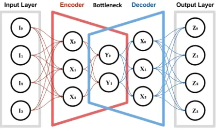
Autoencoders (AE) are a type of neural network that aims to reconstruct data from the input layer into the output layer with a minimal amount of distortion [62]. Since the objective function is calculated with a comparison between the input and output, autoencoders are an unsupervised learning algorithm, since they don’t require class labels to be trained.

An AE is composed of an encoder, a decoder and a bottleneck layer. The function of the en-coder is to compress the input to a more compact representation, which is present in the bottleneck layer, and the function of the decoder is to reverse this compact representation back to the original one. The bottleneck layer connects the encoder and the decoder (figure2.1), and possesses less neurons than the input and output layers. This prevents the network from perfectly copying the input layer to the output layer, and forces it to generalize. The compact representation of the data in the bottleneck layer is also often more robust to signal noise [62].

Figure 2.1: Scheme of a basic autoencoder.

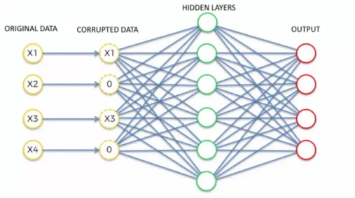
2.1.2.2 Denoising Autoencoders

Denoising autoencoders (DAE) are an extension of regular autoencoders, which are used mainly to remove noise from the input, instead of obtaining a simpler representation, as do normal AEs [69]. This is achieved is by initially corrupting the data before feeding it to the input layer during training process. This corruption can be done through a multitude of ways, such as setting random features to 0, or applying gaussian noise (noise following a normal distribution). After the network makes its prediction, the loss function is calculated in respect to the original data (not to the corrupted sample), which trains the network to reconstruct the original input. Since the network is thus

(28)

often incapable of perfectly reconstructing the inputs because of the noise, a larger hidden layer can be used(figure2.2), which allows the capture of noise robust features, representing the joint distribution of the inputs for a more precise reconstruction.

Figure 2.2: Scheme of a denoising autoencoder.

On this dissertation, denoising autoencoders were used to perform detection of adversarial examples, as these are many times considered normal samples with noise added, and DAEs have the potential to partially remove this noise.

2.1.2.3 Generative Adversarial Networks

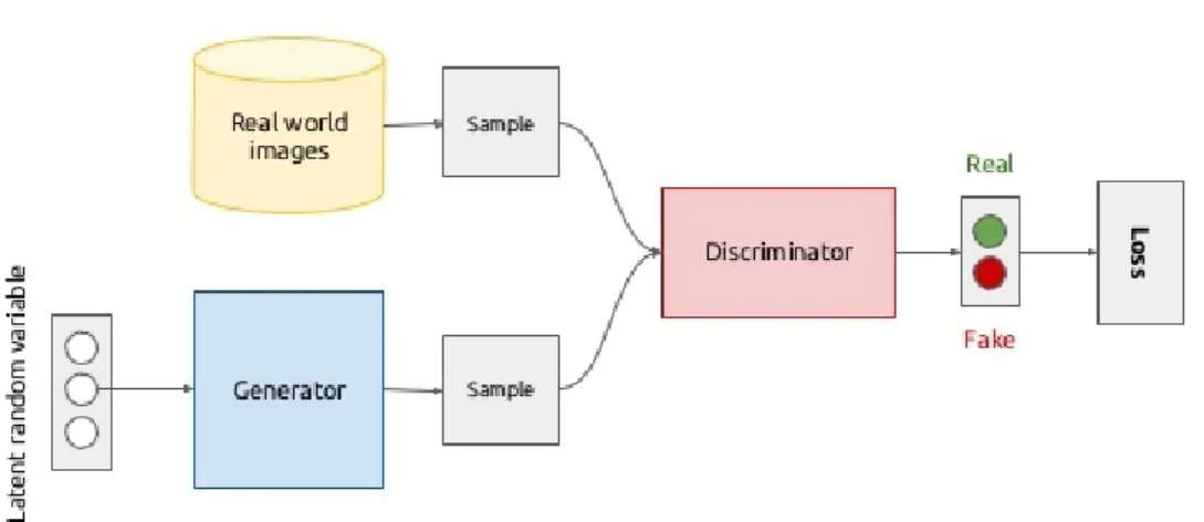
Generative adversarial networks consist of two neural networks that are matched against each other [57]. One of the networks, called the Generator, produces samples by multiple possible means, such as by introducing noise to valid samples, or producing them from scratch using only a random latent variable as seed. The other network, called the Discriminator, receives real samples and adversarial samples created by the Generator, and tries to distinguish them. A loss function is then calculated based on the predictions of the Discriminator, which is then used to adjust the weights of both the Discriminator and the Generator (figure2.3).

In essence, the two networks are playing a game, by improving each other through competi-tion: the Generator tries to create samples that will deceive the Discriminator, and the Discrimina-tor tries to correctly classify the samples, and a single loss function is used to train both models.

One of the biggest problems with regular GANs is that using exclusively gradient descent to train the networks often leads to mode collapse to a parameter setting, always emmitting the same point [50]. So, the optimization becomes highly unstable [28]. Wesserstein GANs were introduced as a means to solve this problem. Instead of using the gradient of the loss function of the neural networks to train the models, they used the Wesserstein distance, also known as the Earth-mover

(29)

Figure 2.3: The general flow of a GAN. Only one loss function is used, which is be used to train both the generator and the discriminator.

distance, which measures the distance between two distributions [28]. This technique was shown to eliminate many of the shortcomings of vanilla GANs, providing a smoother training [28].

2.1.3 Transfer Learning

Transfer learning is an area of machine learning which focuses on the transfer of knowledge be-tween models. This range of techniques is especially useful in computer vision, where training a new neural network from scratch can prove a very expensive task, and by reusing networks pre-viously trained in other tasks, a lot of time and computing power is saved, with minimal loss in the final performance. This takes advantage of the sequenciality in the abstraction of features that occurs in neural networks. The first layers represent simpler features, such as edges and simple shapes, and the last layers represent more complex forms. When both tasks are similar in nature (e.g. image recognition), the first layers can be re-utilized.

Distillation is a technique initially designed to train a neural network with knowledge extracted from another neural network, with the intent of reducing the computational complexity of the classifier in order to deploy it in more constrained devices, such as smartphones, or other devices without fitting hardware [53].

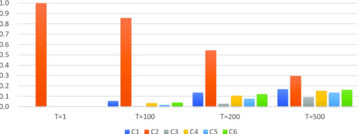
The process of Distillation consists of creating a new simpler network that mimics a teacher network, by approximating its output to the output of the teacher network (the loss function of the learning network is a comparison between its output and the output of the teacher). The problem is that, on a vastly trained teacher network, the class distribution will be very uneven, and the correct classes will have very high values, while the wrong ones will be close to 0, which results in an output that exclusively represents the ground truth labels. A new concept is then introduced called Softmax Temperature, that softens the output of the teacher model, distributing it more

(30)

evenly throughout other classes, facilitating the training process for the learning network (figure 2.4), since it facilitates learning the classes distributions for inputs.

Figure 2.4: Distillation: Softmax temperature illustrated.

Distillation can be used to create more robust classifiers to adversarial examples, as will be later explored.

2.2 Performance Metrics

Evaluating the performance of a classifier is an essential factor on any project. Several metrics have been proposed to evaluate the performance of models, with each having its advantages and disadvantages [54].

2.2.1 Classification Metrics

Classification is the process of identifying the set categories to which a certain sample belongs to, such as identifying if a connection is malicious or not. There are a wide variety of metrics that can be used to evaluate the performance of a classifier, each with its advantages and disadvantages.

Confusion matrixes can be used on binary classification problems, and give us numerical val-ues of the predictions of the classifier, with the diagonal containing the correct predictions, and other cells containing failed predictions (table2.1).

Table 2.1: Confusion Matrix

Predicted Positive Predicted Negative Actual Positive Number of True Positives Number of False Negatives Actual Negative Number of False Positives Number of True Negatives

Accuracy is the simplest form of evaluation, and consists of the ratio of correct and total predictions.

(31)

Accuracy=Correct predictions Total Predictions

Its result is easy to interpret, but it can often be misleading when the ratios between different classes are very different.

For example, if there are 98 samples of one class, and 2 of another class, and the classifier predicts all 100 at being from the first class, we will achieve an accuracy of 98%, which can be misleading because it doesn’t indicate that the model is effective, since all it did was predict the first class for every sample.

Error rate is similar to accuracy, but instead measures the ratio of incorrect and total predici-tons.

Error rate=Incorrect predictions Total Predictions

Sensitivity, also known as True Positive Rate, refers to the fraction of positive samples that are correctly classified. Specificity, also known as True Negative Rate, measures the fraction of negative samples that are correctly classified.

Sensitivity= True Positives

True Positives+ False Negatives

Speci f icity= True Negatives

True Negatives+ False Positives

Precision indicates the fraction of positive samples from all the samples predicted as positive by the model. Recall indicates the fraction of positive samples that are correctly classified from all the correclty classified samples.

Precision= True Positives

True Positives+ False Positives

Recall= True Positives

True Positives+ True Negatives

F1 represents the a weighted average between Precision and Recall, and is calculated with the harmonic mean between Precision and Recall.

F1 = 2 ∗ ₁ 1

Precision+ 1 Recall

(32)

Area Under Curve (AUC) is a popular evaluation metric which combines TPR (also known as Sensitivity) and FPR into one value.

The value of AUC is obtained by plotting the TPR against FPR, producing the Receiver Operat-ing Characteristics (ROC) curve, and calculatOperat-ing the area under the curve, and the main advantage over accuracy is that it is scale invariant.

2.2.2 Performances Comparison

There have been proposed several techniques to compare the performance of two or more algo-rithms across different datasets [70]. For this dissertation, we chose to use the Friedman Test, since its non-parametric.

The test consists of ranking each algorithm for every testing dataset, followed by averaging out the ranks for each algorithm. The Nemenyi Test can be performed afterwards to test if we reject the null hypothesis which states that two algorithms have similar performance. This can be performed by computing the critical difference (CD):

CD= qk(k + 1) 6N

Here, q is a pre-computed critical value for a certain confidence level (we used 95%), k is the number of classifiers, and N is the number of testing sets. If the difference between the average ranks of two classifiers is above the critical difference, we can reject the null hypothesis for that pair.

2.3 Adversarial Machine Learning

Adversarial machine learning comprises a group of techniques that aim to produce malicious in-puts that cause models to misclassify them.

In this section we will explore theory and taxonomies on adversarial machine learning, along with adversarial attack and defense strategies.

2.3.1 Fundamentals of Adversarial Machine Learning

Huang. proposed a formal taxonomy in order to model an attack in adversarial environments [64], introduced models for the adversaries knowledge about the system, and analyzed application-specific factors.

According to the taxonomy proposed, an attack can be classified by the following properties: • Influence - refers to the influence the attack has over the training data. It can either be

a Causative attack if it can influence the training data of the classifier (Poison attacks), or Exploratory, if the attack only aims to probe the training data in order to obtain information that can prove useful in the process of the attack.

(33)

• Security Violation - refers to the violation that the attack aims to achieve. These can be Integrity attacks when the aim is for the attack to be classified as normal (False Negative), Availability attacks, when the aim is to cause classification errors of any type (False Nega-tive or False PosiNega-tive) , rendering the model useless, or Privacy attacks, when the aim is to obtain information from the learner, violating the users privacy.

• Specificity - refers to target of misclassification. These can be Targeted attacks when the intent is for the attacks to be misclassified into a certain class/group of classes, or Indis-criminate when there is no specific class to be targeted, and the objective is only to cause any False Negative.

Furthermore, an analysis of the knowledge the attacker can have over the system is also im-portant for the detection system. Knowledge of the underlying model can provide the adversary with means to exploit the system and make informed decisions. The knowledge of the underlying system can be formalized into:

• Machine learning algorithms - refers to the knowledge of the algorithm(s) used by the detection system.

• Data source - the knowledge of the source of the training data used to prepare the classi-fier(s).

• Data - knowledge of the exact data used to train the classifier(s). • Feature Selection - choice of features for the models.

• Output - refers to the knowledge the attacker has over the output by the classifier over certain inputs.

Overall, the attacks can be classified has white-box attacks or black-box attacks, depending on the knowledge the attacker has over the system. This can be an important information, as lack of knowledge of the system imposes restrictions on the techniques an attacker can use to generate adversarial attacks.

Another limitation that must also be considered when preparing a detection system are the limitations of the application and the environment. These limitations are expressed in the features used in the classifiers. Features are the variables that represent the world space and can be used by the classifier to perform evaluations. Several limitations can arise when an adversary attempts to manipulate features in order to deceive the classifier. These can be organized as:

• Domain Limitations - refers to the limitations an attacker faces when interacting with an application domain, which includes how the user can interact with the application, and what features can realistically be changed by the attacker. For example, when a classifier is used exclusively by an individual to detect spam email, an assumption can be made that the user will not willing-fully corrupt the data in order to deteriorate the classifier.

(34)

• Contrasting Feature Spaces - these refer to the limitations an attacker faces when altering features. Depending on the domain, there are different limitations to how an attacker can alter the features. The attacker might be able to alter a wide variety of features (e.g. in-cluding or not a word in an email), while being limited in altering others (e.g. faking spam email addresses as real ones). There is also a limitation on how much the attacker can alter a certain feature. For example, during a Denial of Service attack, if the time between packets is too long, the attack might prove ineffective.

• Contrasting Data Distributions - refers to the limitation that appears in the conflict be-tween the distributions of data from an adversarial input and a regular input. Certain fea-tures regularly follow certain distributions, and when the adversarial input doesn’t fit them, it is more easily flagged. For example, in the detection of spam emails, the distribution of words of regular emails follows the same pattern as the most used words globally. When an attacker forges adversarial emails, he is limited in the choice of words, by not being able to use many unconventional ones, as they are more easily flagged.

2.3.2 Adversarial Attacks

Several adversatial attack techniques have been proposed, with a trade-off on performance, com-plexity, computational efficiency and application scenario (black-box and white-box).

In white-box attacks, the attacker has knowledge over the training data, model parameters, and other useful information about the classifier. In black-box scenarios, the attacker has little to no knowledge of the classifier, and thus is severely limited.

Most of the attack methods presented were only tested on image domains, but most can equally be applied to tabular data, such as an intrusion dataset, since they are not data dependant attacks, and a feature normalization step can squeeze features to a certain interval, much like the range of available values of each pixel on an image, creating a similar scenario to images. This poses a security threat if an attacker can manipulate multiple features used by the classifiers, allowing the application of adversarial attacks to manipulate intrusions or malware to go undetected by the classifiers.

Gradient based attacks typically introduce perturbations optimized for certain distance metrics between the original and perturbed samples. The three mainly used distance metrics in literature are:

• L∞- minimize the maximum amount of perturbation introduced to any feature of the sample;

• L0- minimize the amount of features perturbed of the sample;

• L2- minimize the Euclidean distance between original and adversarial samples.

(35)

Table 2.2: Datasets used in literature review.

Name Type

MNIST [7] Handwritten numbers

GTSRB [4] Traffic Signs

CIFAR10 [2] Object recognition

NSL-KDD [51] Instrusion dataset

Kaggle Microsoft Malware Classification Challenge [6] Malware dataset

2.3.2.1 Limited-memory Broyden–Fletcher–Goldfarb–Shanno Attack

Szegedy et al. proposed one of the first gradient methods to generate adversarial examples using box constrained Limited-memory Broyden–Fletcher–Goldfarb–Shanno (L-BFGS) optimiza-tion [59]. Given an input image, this method searches for a different image that is similar to the first, under L2distance, that is mislabeled by the classifier. By adding noise to the original image,

the problem can be represented as a minimization problem, where the objective is to minimize the distance between the original image and the adversarial one:

min||r||2sub ject to: f(x + r) = l

Here, x is the original image, r is the perturbation, f is the loss function of the classifier and l the incorrect prediction/label. Since this is a non-trivial problem, the authors approximate it by using L-BFGS optimization algorithm to solve it (the box constraint is needed to limit the possible values of the variables, which are pixels in image scenarios). Although this method is effective at producing adversarial examples, it is impractical, since it uses a computationally expensive algorithm to search for an optimal solution.

2.3.2.2 Fast Gradient Sign Method Attack

Goodfellow et al. proposed a simple and fast gradient based method to generate adversarial exam-ples called Fast Gradient Sign method (FGSM) [52], with the aim of minimizing the maximum amount of perturbation added to any pixel (L∞distance metric) of the image to cause

misclassifi-cation. The rationale of this technique is to compute the gradient of the loss function with respect to the input (e.g. using backpropagation), and alter the existing data by adding a perturbation ε with the sign of the gradient. The formula for the attack is the following:

η = ε ∗ sign(∇x J(θ , x, y))

where η is the perturbation, ε is a hyper-parameter controlling the magnitude of the attack, J is the cost function, ∇x is the parameters of the model, x the input and y the target label (Figure

(36)

2.5). By increasing the value of ε , the magnitude of the attack becomes greater, but the image will become more noticeably distorted.

Figure 2.5: FGSM - By using a ε of 0.007, which only allows at most 1 bit to be changed in a 8 bit representation of each channel of a pixel, the perturbation can lead to a misclassification.

Although this method is less effective than other state of the art techniques for generating adversarial attacks and is noticeable to humans, it is one of the most efficient at computing time, allowing fast generation of adversarial examples.

2.3.2.3 Jacobian Based Saliency Map Attack

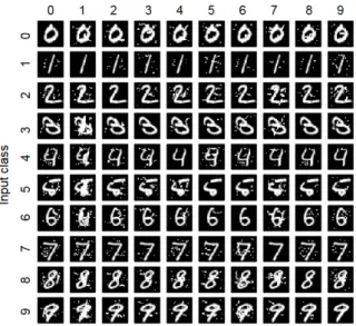
Papernot et al. proposed a new adversarial sample generation technique called Jacobian based Saliency Map Attack (JSMA) [56], that uses feature selection, unlike the previous methods, with the aim of minimizing the number of pixels modified (L0distance metric) while causing

misclassification.

This method revolves around the computation of saliency maps for an input sample, which contain the saliency values for each input feature. These value indicates how much the modifi-cation of that feature will perturb the classifimodifi-cation process, and is different for each target class. The features are then selected in decreasing order of saliency value, and each is modified accord-ingly by θ. The process finishes when misclassification occurs, or a threshold number of modified features is reached (figure2.6).

We can conclude that, compared to FGSM, this method is able to generate adversarial inputs with similar success rate, but vastly less feature modification, at the expense of higher computing cost.

2.3.2.4 Deepfool

Moosavi-Dezfooli et al. proposed an untargeted adversarial sample generation technique called DeepFool [55], with the aim of minimizing the euclidean distance between perturbed samples and original samples (L2 distance metric).

(37)

Figure 2.6: JSMA on MNIST dataset. The original samples are found in the diagonal, with all other elements being adversarial examples.

The generation of the attack consists of the analytical calculation of a linear decision boundary that separates samples from different classes, followed by the addition of a perturbation perpen-dicular to that decision boundary (figure2.7).

Figure 2.7: Deepfool - a sample x0 is added a perturbation r in the direction of the hyperplane that separates the original class and the target class.

In neural networks, these decision boundaries are almost always not linear, so they add the perturbations iteratively by performing the attack multiple times, finishing when an adversary is found . The overshoot parameter is used as a termination criterion to prevent vanishing updates. Although this method allows the generation of adversarial samples with less perturbations than

(38)

FGSM and JSMA, and with higher misclassification rate, it is more computationally intensive than both.

2.3.2.5 Carlini & Wagner Attack

Carlini and Wagner created a new attack based on the L-BFGS attack, called Carlini & Wagner attack (C&W) [30], by representing the attack as an optimization problem. Instead of directly using the loss function in the optimization process, the authors propose other objective functions, study different distance functions for each of the three distance metrics, and test other optimizers that don’t use box constraints by using the hyperbolic tangent (tanh) to find the optimal pertur-bations in the specified ranges. The authors observed that the attack was able to defeat multiple adversarial defense techniques, such as defensive distillation.

2.3.2.6 Generative Adversarial Networks

Generative Adversarial Networks (GAN) have also been used to generate adversarial attacks. Chaowei Xiao et al. created a modified version of GANs called AdvGAN[23], and were able to successfully generate adversarial examples. Instead of only having a generator and a discriminator, the authors also included the target classifier, or an approximated version of it using transfer learning, on the GAN. They then used the sum of the loss functions of the discriminator and the classifier to create one loss to be used to train the generator. Both losses are used because the loss of the discriminator indicates how far the generated samples are from the real samples, forcing the generator to add smaller perturbations, while the target classifier loss is used to evaluate the success of the misclassification of those samples (figure2.8).

Figure 2.8: Structure of an AdvGAN. The loss function used to train the generator is the combi-nation of the loss of the discriminator and the loss of the target classifier.

Although the generation of adversarial samples with GANs is effective, the distribution of the perturbations is more unpredictable than the previously mentioned gradient based methods, which all introduce perturbations under a certain distance metric, and the generation can also be highly unstable, even for Wesserstein GANs [12].

(39)

2.3.2.7 Zeroth Order Optimization Attack

Zeroth-order Optimization attack (ZOO) was proposed by Chen et al. [32], and allows the esti-mation of the gradient of the classifiers without access to the classifier, which is ideal for a black box attack. The method consists of iteratively adding perturbations to each feature of the samples and querying the classifier to estimate its gradient and Hessian of these different features. This makes it an oracle based technique, not requiring the training of substitute models, and the at-tacker doesn’t require information on the classifier. Although this method was proven effective at estimating the gradient, it can require a large amount of queries to the oracle, which can be used to detect the attacker.

2.3.2.8 Transferability of Adversarial Attacks

Goodfellow et al. explored an interesting property of adversarial inputs, which is transferability across models [52]. The authors observed that, when an adversarial input is successfully misclas-sified by a model, it will often be misclasmisclas-sified by other models, even when they have different arquitectures or were trained in different datasets. It was also observed that they often agree on the predicted class. This allows an attacker to perform black-box attacks by training their own substitute model, either by using transfer learning techniques or training on the same dataset, and using that model to generate adversarial samples that can target that classifier [49].

2.3.3 Adversarial Defenses

There are a wide variety of approaches that can be taken to make classifiers more resilient to adversarial attacks. These countermeasures can follow two approaches [42]:

• Reactive Defenses: focus on detecting adversarial examples separately from an already trained classifier;

• Proactive Defenses: focus on building classifiers that are robust to adversarial examples. 2.3.3.1 Adversarial Training

Goodfellow et al. proposed Adversarial Training [52], the first proactive defense method to improve resilience to adversaries which consists of including adversarial examples in the training set. Instead of directly including adversarial examples in the training set, the authors propose the usage of an adversarial objective function, which replicates the same effect. The formula used by the authors is the following:

˜

J(θ , x, y) = α ∗ J(θ , x, y) + (1 − α) ∗ J(θ , x + sign(∇xJ(θ , x, y)))

Here, ˜J is the final objective function, which is the sum of the loss on the normal sample and the loss on an adversarial sample using FGSM, with αcontrolling the influence of each loss function on the final loss.

(40)

The authors concluded that this technique was effective at regularizing the classifier, although misclassifications still occured. The main disadvantage of this method is that it needs to be trained against specific types of attacks to be resilient to them, being mostly effective against Linfattacks,

such as FGSM [37]. The authors were able to reduce the error rate from 89.4% to 17.9% using adversarial training against FGSM on the MNIST dataset [52]. Swami et al. further explored this technique by showing superior effectiveness when introducing perturbations on intermediate layers of deep neural networks instead of the input layers [40].

2.3.3.2 Gradient Masking

Gradient Masking comprises a group of proactive defensive techniques which assume that "if the model is non-differentiable or if the model’s gradient is zero at data points, then gradient based attacks are ineffective"[14].

One form of gradient masking is Gradient Hiding, which consists on using non differentiable models to perform classification, such as Decision Trees. This prevents the adversary from esti-mating the gradient and using it to generate adversaries.

Gradient Smoothing comprises a range of techniques that smooth out the model’s gradient, causing numerical instabilities which make the estimation of gradient more difficult.

Although the objective of preventing the adversary of estimating the gradient was achieved, Papernot et al. concluded that, both under black-box and white-box scenarios, the training of sub-stitute classifiers to estimate the gradient is an effective technique to generate adversaries because of the transferability property, making gradient masking a ineffective defense technique [47], [48].

2.3.3.3 Defensive Distillation

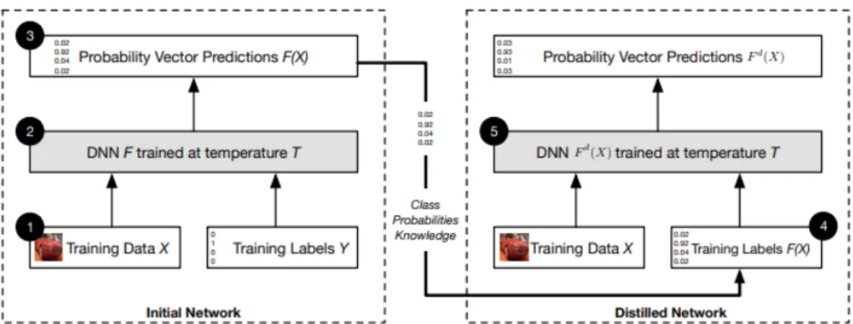
Another proactive defense technique was proposed by Papernot et al. called Defensive Distilla-tion [46]. The authors propose the usage of distillation as a means to improve the robustness of a classifier to adversarial inputs. Instead of using distillation in the conventional way to train a different, simpler model from a teacher model to allow deployment on resource constrained de-vices, it is proposed to use the knowledge extracted during the distillation process to improve the classifier itself at detecting adversarial samples. By increasing the temperature at which a network is trained on the softmax layer, the teaching network outputs have less confidence on the ground truth label and show a higher distribution across classes. It is then proposed to use this output to train a second network with the same structure as the first. The structure is not changed since the objective is to make the network more resilient, and not more computationally efficient. The au-thors observe that, by using the entropy generated in the softmax layer to train the same network, it will become more resilient to adversarial samples, as it prevents the network from fitting too tightly to the ground truth class labels. An overview on the proposed technique is in figure2.9.

To test the proposed method, the authors used MNIST and CIFAR10 datasets, and the results showed that distillation reduces the success of adversarial samples from 95.89% to 0.45% on the

(41)

Figure 2.9: Overview of defensive distillation technique. A neural network F was initially trained and performed predictions under a certain temperature T. The predicted labels distribution is then used to train a second neural network with the same , which is theorized to be more resilient to adversaries.

MNIST dataset, and 78.9% to 5.11% on the CIFAR10, with variations of accuracy in the detection of normal samples in the range of -2% and 2%.

2.3.3.4 Feature Squeezing

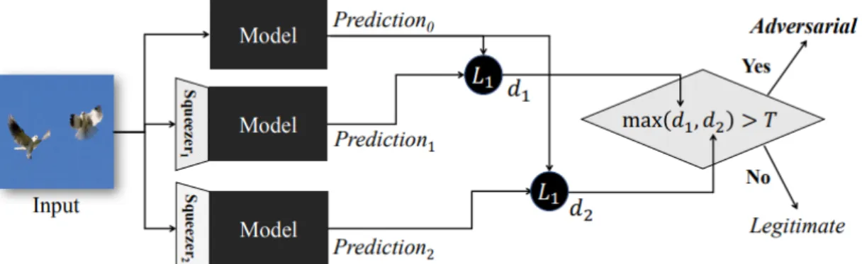
Weilin Xu et al. proposed Feature Squeezing [41] as a means to combat adversarial examples. The intuition behind this technique is to compress the features of the sample (the pixels of the image in their case) and perform classification on the compressed sample. If the prediction by the classifier on the compressed sample is substantially different from the prediction of the original sample, it is considered an adversarial example. The authors tested several compression methods, namely Bit depth compression, Median Smoothing and Non local means, but found that the best method was largely dependent on the dataset. An overview of the feature squeezing framework can be seen in figure2.10.

This technique was proven effective on MNIST, CIFAR10 and ImageNet datasets against many state of the art adversarial attacks, such as FGSM, JSMA, Deepfool and C&W under different distance metrics, showing an improvement between 20% and 70% on the detection rate for all datasets, with Bit Depth squeezing being the most effective on the MNIST dataset and Median Smoothing the most effective in CIFAR10 and ImageNet.

2.3.3.5 Transferability Block

Hossein Hosseini et al. proposed a new proactive technique to block the transferability of adver-sarial examples across different models on black-box environments[35].

It was previously shown that adversarial examples crafted to target a specific classifier often work on different classifiers, even if their training data or architecture are different. Instead of

(42)

Figure 2.10: Framework of feature squeezing. When the difference of predictions on different models using different/no squeezers exceeds a threshold, the input is considered adversarial.

trying to create a defense mechanism that assigns adversarial examples to their original label, the authors propose discarding adversarial examples, by creating a new class called NULL, which indicates if the input is suspicious.

The authors start by training a classifier exclusively with clean data. After the initial training, they compute a function that outputs the NULL probabilities, which represent the probability of a sample being adversarial based on the amount of perturbations present. They introduce per-turbations using a brute-force method, which iteratively modifies certain features, and repeat this process for multiple number of features perturbed. The third and final step is to perform adversarial training, and deciding the label based on the NULL probabilities (figure2.11).

Figure 2.11: Transferability defense: instead of assigning a larger credebility to the target class during training, the network is trained to assign it to the NULL label, proportionally to the magni-tude of the perturbations.

(43)

Although this method is not intended to identify the true label of a certain adversarial sample, it is one of the most effective techniques in literature at identifying adversarial examples.

The results show the transferability rate of different attacks on the MNIST and GTSRB datasets reduced from over 55% to less than 6%.

2.3.3.6 Universal Perturbation Defense Method

Naveed Akhtar and Jian Liu proposed the Universal Perturbation defense method as a defense method against adversaries [25]. The method consists of placing a Perturbation Rectifying Net-work(PRN) before the input layer of the target classifier. This network is trained using images with and without perturbations, and the layers of the classifying network frozen. This process creates a network that is effectively denoising the inputs and, by evaluating the difference on the inputs and the outputs of the PRN, extracts discriminative features, which are used to train a binary classifier that is able to identify an adversarial sample. The results on the GoogleNet dataset show that the detection rate of adversarial attacks was between 91.6% and 97.5%, both against Linfand

L2 attacks.

2.3.3.7 MagNet

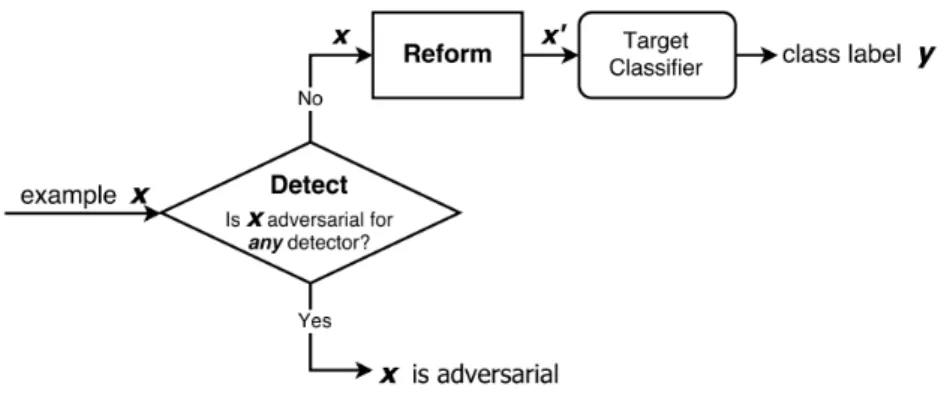
Dongyu Meng and Hao Chen proposed a defensive framework called MagNet [38]. The frame-work consists of two main modules: a detector and a reformer.

The authors consider that a classifier misclassifies an adversarial attack for two reasons: the example is distant from the boundary of the manifold of the normal examples, or the example is close to the manifold of normal examples, but the classifier doesn’t generalize well.

Figure 2.12: MagNet defense strategy. Using an ensemble of detectors, if any considers a sample to be adversarial, it is considered to be adversarial, removing samples with high magnitude per-turbations. Regular samples and adversarial samples with small perturbations are then directed to the reformer, which denoises the data and directs it to a classifier that performs predictions.

The purpose of the detector is to defend against the first case (adversarial examples distant from the manifold), and it is built using an autoencoder. The autoencoder is trained on normal

(44)

samples, and during deployment, it rejects samples that deviate substantially from the manifold. It does this by verifying the loss function, which is the mean squared error, and rejects samples with an error above a threshold, which was in this case the maximum loss observed during training.

The reformer then receives samples that were classified as normal by the detector, and "de-noises" the inputs, to remove small perturbations that were not caught by the detector, and approx-imate the adversarial samples to normal samples. The output of the reformer is then input on a classifier, which will perform classification among the normal classes.

The authors tested the proposed technique on the MNIST and CIFAR datasets, using FGSM, IGSM (an iterative variation of FGSM), DeepFool and C&W. All attacks were effective at de-creasing the performance of the classifiers, with C&W being the most effective by reducing the accuracy to 0%, and DeepFool to 19.1%. After deploying the defense, all accuracies improved, with all being above 92% on the MNIST dataset, and above 77.5% on the CIFAR dataset.

2.3.3.8 Separate Binary Classifier

Zhitao Gong et al. proposed an alternative to adversarial training which consists of training a sep-arate classifier to exclusively detect adversarial examples [33]. Since the authors didn’t formally name the proposed defense, we use the term "Separate Binary Classifier" to identify it. Instead of including adversarial examples on the training set, and training the classifiers to detect the orig-inal label of the adversarial examples, the authors propose training a separate binary classifier to detect if a sample is adversarial or not. Samples that are considered adversarial are ignored, while samples considered clean are passed on to a classifier trained on normal samples. The main ad-vantage of this technique over adversarial training is that it serves as a pre-processing step, not requiring modifications on an already trained model, making it easy to deploy.

After testing the technique on MNIST and CIFAR datasets, while attacking them with FGSM attack, the authors achieved over 99% accuracy on both datasets, although when they tested on perturbations with smaller magnitude than the ones present in the training set, the accuracy dras-tically dropped to 0.003%, meaning that there is a limitation on the generalization of the model, which the authors argued is also a problem in adversarial training and distillation.

2.4 Conclusions

The initial part of our experiments is to use regular classifiers to perform classification on normal and adversarial data. To do this, we chose to use at least one classifier from each tribe according to Pedro Domingos [13]: Decision Tree, Random Forest, Naive Bayes, Support Vector Machine, Neural Network and a Denoising Autoencoder combined with a Neural Network. We didn’t include evolutionary algorithms since those are not optimal to perform classifications.

To generate adversarial attacks, we decided to use at least one attack for each distance metric: Fast Gradient Sign Method, Jacobian Based Saliency Map Attack, Deepfool and Carlini & Wagner Attack. We included C&W to test its effectiveness against distillation defense, since it was claimed by the authors that this attack could defeat it.

(45)

Finally, we decided to use four defense strategies: Adversarial Training, Separate Binary Classifier, MagNet and Defensive Distillation. In this selection we were more constrained, since most other defenses, such as Feature Squeezing, are more specific to image scenarios.

(46)

(47)

Chapter 3

Literature Review

In this chapter, we explore different works that have applied adversarial machine learning to intru-sion and malware detection scenarios. We didn’t specify our search to Denial of Service contexts, since there are very few works that apply adversarial machine learning specially to this case, and because these scenarios are very similar in application of the strategies. The search was performed on multiple science databases, such as IEEE Xplore, Springer, arXiv, ScienceDirect and Re-search Gate, as well as regular Re-search engines such as Google, using the keywords "Intrusion Detection", "Malware Detection" and "Adversarial Machine Learning". We selected all articles found on intrusion detection, and selected the most cited on malware detection.

Maria Rigaki and Ahmed Elragal first tested the effectiveness of adversarial attacks in an intrusion detection scenario [39]. The authors performed tests on the NSL-KDD dataset [51], by using FGSM and JSMA to generate Targeted attacks, and used 5 models to perform classification: Decision Tree, Random Forest, Linear Support Vector Machine, Voting ensembles of the previous three classifiers and a Multilayer Perceptron. The results on JSMA showed that all classifiers accuracy was affected, with Linear SVM being the most substantial one with a drop of 27%. The drop on F1-score and AUC was also notable, especially on the Linear SVM and Voting ensemble. Overall, the most resilient classifier was Random Forest, which suffered smaller performance drops across all metrics, with a drop of 18% on the accuracy and 6% on the F1 score and AUC. The authors made an important remark on the percentage of features modified by the attacks: FGSM modifies 100% of the features on every sample, while JSMA only modified on average 6% of the features. This makes JSMA a more realistic attack, since in the field of intrusion detection, there are domain specific limitations to the attacker relating to what features he can modify, which is coherent with the taxonomy of Huang et al. [64]. It was also noted that, although the explored attacks proved their effectiveness against unknown classifiers, they still required knowledge about the preprocessing of the data, such as the features used for classification, and the effectiveness of attacks under other circumstances was not tested.

Zheng Wang also tested the performance of adversarial attacks on the NSL-KDD dataset [51], using four different adversarial attack techniques to attack a Multi Layer Perceptron classifier