Hedging of barrier options

Diogo Monteiro da Costa Soares Justino

Master in Finance

Thesis Supervisor:

Prof. João Pedro Nunes, Associate Professor, ISCTE Business School, Department of Finance

As opções com barreira são opções exóticas cuja gestão do risco pode ser difícil de executar devido à possibilidade de o delta e gamma serem muito elevados nas imediações da barreira. Esta tese procura investigar alternativas para a gestão do risco deste tipo de opções que minimizem os ganhos e perdas da estratégia dinâmica conhecida por delta hedging.

Investigamos duas metodologias propostas por Carr (1994) e Derman (1994) que constroiem portfolios estáticos com várias opções vanilla. A primeira envolve uma relação designada por simetria put-call e usa opções com a mesma maturidade e diferentes preços de exercício. A segunda divide o tempo em vários intervalos e procura replicar o valor da opção na barreira através de outras opções com diferentes maturidades.

As estratégias são avaliadas num ambiente de movimento Browniano geométrico e em dados reais do índice S&P 500.

Palavras-chave: Black-Scholes-Merton, Opções com Barreira, Delta Hedging, Static Hedging Classificação JEL: G12, G13

Barrier options are exotic options that can be difficult to hedge due to the possibility of the delta and gamma values being very large close to the barrier. This thesis investigates methods to hedge barrier options that can minimize the profits and losses that arise when using a dynamic technique known as delta hedging.

We present two methods by Carr (1994) and Derman (1994) that create a static portfolio of vanilla options. The first method uses the put-call symmetry relationship and builds a portfolio of different options with the same maturity and different strikes. The second method divides time into intervals and tries to match the barrier option payoff at each of theses intervals with other vanilla options. The techniques are evaluated in the geometric Brownian motion environment where they were deduced and in real market conditions with time series of the S&P 500 index.

Keywords: Black-Scholes-Merton, Barrier Options, Delta Hedging, Static Hedging JEL Classification: G12, G13

To my family. Mom, dad, grandma, grandpa, and those living in our hearts. To Sara, for your support.

S – asset price K – exercise price H – barrier price R – rebate

r – risk-free interest rate q – asset yield

t – time instant T – ending time

Resumo...I Abstract...II Acknowledgements...III Notation...IV 1 Introduction...1 2 Theoretical Background...3 2.1 Options...3 2.2 Black-Scholes-Merton Model...3 2.3 Barrier Options...6 2.4 Relationships...7 2.5 Restricted Distribution...8 2.6 Pricing formulas...10 2.6.1 Down-and-in Call...12 2.6.2 Up-and-in Call...12 2.6.3 Down-and-in Put...13 2.6.4 Up-and-in Put...13 2.6.5 Down-and-out Call...14 2.6.6 Up-and-out Call...14 2.6.7 Down-and-out Put...15 2.6.8 Up-and-out Put...15 2.7 Greeks...16 2.7.1 Delta...16 2.7.2 Gamma...18 2.7.3 Theta...19 2.7.4 Vega...20 2.7.5 Rho...20 3 Hedging...21 3.1 Delta Hedging...21 3.2 Put-Call Symmetry...25 3.3 Boundary Replication...30 4 Experimental Results...40

4.1 Geometric Brownian Motion...40

4.1.1 Delta Hedging...41 4.1.2 Put-Call Symmetry...42 4.1.3 Boundary Replication...44 4.2 Market Data...46 4.2.1 Delta Hedging...47 4.2.2 Put-Call Symmetry...49 4.2.3 Boundary Replication...50 5 Conclusions...53 6 Bibliography...54

1 Introduction

In recent years, the use and importance of derivatives, financial instruments whose value depends on the value of other underlying variables, has grown enormously as mathematical models to value them appear and more research is devoted to their study. Derivative contracts are widely traded on many exchanges throughout the world and in the over-the-counter market where financial institutions trade between them and some of their biggest clients. Many of this institutions now employ mathematicians, statisticians, physics and engineers to handle the complex mathematics behind many derivatives. Their job is to trade, value and analyse the risk to the financial institution of trading derivatives.

Options are one type of derivative contract that provide their buyer a right and their seller an obligation. They can be categorized as non-linear derivatives, as their value is a non-linear function of the underlying asset price, and further divided between standard, also termed vanilla, and exotic options. Exotic options appear as the development of mathematical finance provided financial institutions with the tools to meet different market views of clients apart from the typical upside and downside exposition to a financial asset provided by standard options. Barrier options are one type of exotic options where the payoff depends on whether or not the barrier was breached during the life of the option.

Financial institutions that trade options are often only interested in providing a service to their clients and are not expressing a particular view on some underlying asset. They are left with the task of hedging the risk of the positions assumed which can be a complex procedure because of the non-linear characteristics of options.

One of this procedures follows directly from the derivation of the Black-Scholes-Merton model in Black and Scholes (1973) and Merton (1973) and builds a riskless portfolio of the underlying asset and risk-free securities that is continuously rebalanced. This dynamic hedging technique can be applied to barrier options but is subject to substantial error when the portfolio cannot be continuously rebalanced as is often the case.

To overcome the difficulties of dynamic hedging, static hedging techniques were proposed. In Carr (1994), Carr (1997) and Carr (1998) the authors use a relationship between options of different strikes to create a static portfolio that can be used to hedge barrier options. Derman

(1994) took a slightly different approach by constructing a portfolio with many different maturities that replicates a target option boundary payoff.

An evaluation of this techniques is carried out in this paper. The rest of the thesis is organized as follows:

Chapter 2 provides the theoretical background of options and their mathematics. The Black-Scholes-Merton model is introduced and the eight barrier options are valued under the assumptions of this model. We also introduce the risk measures of barrier options, or greeks, and compare them to the greeks of vanilla options.

Chapter 3 introduces methods to hedge barrier options. The process of dynamic hedging is described and two techniques for static hedging, the put-call symmetry and the option boundary replication, are explained.

Chapter 4 tests the hedging models under computer generated data and real market data. Chapter 5 concludes.

2 Theoretical Background

2.1 Options

Options are contracts where the holder has a right and the seller a liability. A call option gives its holder the right to buy an asset by a certain date at a certain price. A put option gives its holder the right to sell an asset by a certain date at a certain price. The price at which the holder of the option can buy (sell) the asset and at which the seller has to sell (buy) is called the exercise price or strike. The date at which the option rights expire is called the expiration or maturity date. If the holder can only exercise his right at the maturity of the option contract then the option is of the European type. If, on the contrary, the holder can exercise his right at any time before or at maturity, the option it of the American type.

The call option payoff is defined mathematically as

c=max S− K ,0 (1)

where S is the asset price at expiration and K is the exercise price. Similarly, the payoff of the put option is defined as

p=max K −S ,0 (2)

2.2 Black-Scholes-Merton Model

In 1973 a major breakthrough in the pricing of options was achieved. Fischer Black and Myron Scholes in Black and Scholes (1973) and Robert Merton in Merton (1973) were able to model and develop a closed pricing formula for European options. Their work was later recognized with the Nobel prize for economics award.

The Black-Scholes-Merton model develops on the assumption that an asset price follows a geometric Brownian motion with constant drift and volatility, a time, continuous-variable stochastic process also called a generalized Wiener process that satisfies the equation

dS

S =r −q dt dz (3)

where S is the asset price, r is the continuously compounded risk-free interest rate, q is the continuously compounded asset yield, σ is the standard deviation of the return of the asset or annualized volatility and dz is a Wiener process. By definition, dz follows a normal distribution with mean zero and variance rate equal to the time instant dt

With this model for the asset price and using a well known result from stochastic calculus called Itô's lemma, we arrive at the stochastic process followed by a function of the asset price from the stochastic process followed by the asset price itself. From Itô's lemma, the process followed by a function G of S and t when S follows the process defined by (3) is

dG=





Taking into account expression (4) it follows that the process followed by ln S is

d ln S=



2

2



Therefore, the change in ln S between time zero and some future time T is normally distributed lnST S0 ~

[





]

where ϕ(m,v) is a normal distribution with mean m and variance v. Integrating both sides of equation (5) between t and T we have that

S_T=S_texp

[



2



∫

dz

]

Knowing that ln S follows a normal distribution, the price of an asset at future time T given its price today follows a log-normal distribution. The only source of uncertainty is the Wiener

process which is the same for both S and ln S.

We now construct a portfolio of the asset and a derivative f and try to eliminate this source of uncertainty keeping in mind that the derivative f must satisfy equation (4). Defining Π as the portfolio value

=−f ∂ f

∂S S (8)

And taking the discrete versions of equations (3) and (4) results in

 =





which does not involve the source of uncertainty dz. Therefore, the portfolio must be riskless for the period of time Δt and, according to risk neutral valuation, must earn the same as other short-term risk-free securities or an arbitrage opportunity would arise

 =r−q   t (10)

When we substitute equations (8) and (9) into equation (10) we obtain the Black-Scholes-Merton partial differential equation

∂ f ∂t r−q S ∂ f ∂t  1 2 2 S2∂ 2 f ∂S2=rf (11)

This equation has many solutions corresponding to the different derivatives that can be defined on S. If we define the following boundary conditions

{

(12)

and solve the Black-Scholes-Merton partial differential equation we arrive at the following formula for the time zero price of an European option

c=Se−qT_{N  d} 1−Ke−rTN  d2 (13) where d1= ln























and N(x) is the cumulative probability distribution function of the standard normal distribution.

From the put-call parity given by

cK e−rT

=pS e−qT ₍₁₆₎

we obtain the pricing formula for an European put option

p=Ke−rT_{N −d}

2−Se−qTN −d1 (17)

The following assumptions apart from the geometric Brownian motion were made while deriving the pricing formulas for European call and put options:

• It is possible to short-sell the asset with full use of the proceeds; • There are no transaction costs or taxes;

• Securities are perfectly divisible and trading is continuous; • There are no riskless arbitrage opportunities;

• The risk-free interest rate is constant for all maturities and one can borrow and lend at this rate.

2.3 Barrier Options

While the payoff of standard call and put options only depends on the price of the underlying at maturity, barrier options are path-dependent exotic derivatives whose value depends on the

underlying having breached a given level, the barrier, during a certain period of time. The market for barrier options has grown strongly because they are cheaper then corresponding standard options and provide a tool for risk managers to better express their market views without paying for outcomes that they may find unlikely.

We can divide barrier options into knock-in and knock-out options. An European knock-in option is an option whose holder is entitled to receive a standard European option if a given level is breached before expiration date or a rebate otherwise. An European knock-out option is a standard European option that ceases to exist if the barrier is touched, giving its holder the right to receive a rebate. In both cases the rebate can be zero.

The way in which the barrier is breached is important in the pricing of barrier options and, therefore, we can define down-and-in, up-and-in, down-and-out and up-and-out options for both calls and puts, giving us a total of eight different barrier options. There are more complex types of barrier options like double barrier options but we will not cover them in this text.

2.4 Relationships

Suppose that we have a portfolio composed of a down-and-in call and a down-and-out call with identical characteristics and no rebate. If the barrier is never hit the down-and-out call provides us a standard call. If the barrier is hit then the down-and-out call expires worthless but the down-and-in call emerges as a standard call. Either way we end up with a vanilla call so the following relationship between barrier options and vanilla options must hold when the rebate is zero

c=cdicdo (18)

With a similar reasoning we can reach the same relationships for the other barrier options

c=c_uic_uo (19)

p= p_dip_do (20)

2.5 Restricted Distribution

To price standard options in the Black-Scholes-Merton model we used the density function

f  x = 1 



[

]

which results directly from expression (7) and the probability density function of the standard normal distribution. The distribution (22) is the unrestricted distribution of the underlying asset return because no condition on the path of S is imposed.

On the other hand, barrier options are claims conditional on the path of S and, therefore, the distribution of the underlying asset return is restricted. This restriction raises the need for a new density function conditioned on the barrier being breached and leads us to the study of absorbing and reflecting barriers.

An absorbing barrier is a barrier which upon touching all particles vanish thus resembling knock-out barrier options. A reflecting barrier is one in which, as stated by the reflection principle, for every sample path that hits level y before time t but finishes below level x at time t, there is another equally probable path that hits y before time t and then travels upwards at least (y-x) units to finish above level (2y-x).

The variables y and Y will be defined as the, respectively, minimum and maximum rate of return of the underlying asset from time t to time T

y_=min





S_t









S_t





an upper barrier U never being touched is given by 









{





















which is the same as the solution to a Brownian motion with an absorbing barrier. Making use of the identity that expresses the probability that the barrier is never touched and the probability that the barrier is indeed touched







U

S









U

S





we can easily find that the density function of the return of the asset conditional on a upper barrier U being touched is given by











{





















Also in Harrison (1985) the density function of the return of an asset conditional on a lower barrier L never being touched is shown to be given by











{





















and using an expression similar to (27)







S









L

we find that the density function of the return of the asset conditional on a lower barrier L being touched is given by











{





















Looking closer at the density functions we see that we can replace both U and L for a general barrier H without changing the meaning of the formulas.

When pricing rebates for knock-in barrier options we are interested in the density function of the return of an asset conditional on the barrier never being hit. We can only know if this condition holds at the expiration of the option. Thus we can use the previously developed density functions to price the rebate.

In the presence of a knock-out barrier option the rebate is priced differently because the barrier can be breached at any time until maturity. We need a new density function that takes into account the distribution of the first passage time at a particular point which can be shown to be given by 















[









]

This density function works for both up-and-out and down-and-out barrier options as long as we change the sign of the expression.

2.6 Pricing formulas

Merton (1973) and Rubinstein (1991a) derived the following closed formulas for the pricing of European barrier options. They make use of the restricted, unrestricted and first passage time density functions developed in the previous section and the remaining Black-Scholes-Merton model assumptions.

A=Se−qT_{N  x}

B=Se−qT N  x2−Ke −rT N  x2− 























[









]

[









_

]































































where ϕ and η are variables that can be set to 1 or -1.

Note that we can merge expressions (13) and (17) for the Black-Scholes-Merton price of a call and put option respectively to obtain a general vanilla option pricing formula. If ϕ is set to

1 then expression (33) becomes the call option pricing formula from (13). If ϕ is set to -1 the same expression is equal to the put option pricing formula (17).

2.6.1 Down-and-in Call

The down-and-in call option gives its holder the right to receive a vanilla call option if the barrier H is hit or a rebate R otherwise. At inception the underlying price S is higher than the barrier H and has to move down before the regular option becomes active. Expressed mathematically, the payoff function is

c_di=

{

R ∀t≤T : S_tH (45)

When K≥H we value the option using the restricted density function in the interval [K; +∞[. If

K≤H we need to split the integration region and use the unrestricted density function in the

interval [K; H] and the restricted density function in the interval [H; +∞[. The price of a down-and-in call is then given by

cdi=

{

A−BDE K≤ H ;=1 ;=1 (46)

2.6.2 Up-and-in Call

Like the down-and-in, the up-and-in call option gives its holder the right to receive a regular call option if the barrier H is breached or a rebate R otherwise, but the underlying price S starts below the barrier H and has to move up for the regular option to be activated. The payoff function is defined as

c_ui=

{

R ∀t≤T : S_tH (47)

If K≥H the value of the option is simply the value of a standard call option. If, instead, K≤H we use the restricted density function in the interval [K; H] and the unrestricted density function in the interval [H; +∞[. The price of a up-and-in call is then given by

cui=

{

B−C DE K ≤H ;=−1 ;=1 (48)

2.6.3 Down-and-in Put

A down-and-in put option gives its holder the right to receive a standard put option if the barrier H is hit or a rebate R otherwise. The underlying price S starts above the barrier H and has to move down before the vanilla put is born. The payoff function is expressed mathematically by

p_di=

{

R ∀t≤T : S_tH (49)

If K≥H we value the option with restricted density function in the interval [H; K] and the unrestricted density function in the region ]-∞; H]. When K≤H the value of the down-and-in put is the value of a vanilla put option. The price of a down-and-in put is given by

pdi=

{

AE K ≤H ;=1 ;=−1 (50)

2.6.4 Up-and-in Put

The up-and-in put option gives its holder the right to receive a regular put option if the barrier

H is hit or a rebate R otherwise. At inception the underlying price S is lower than the barrier H

and has to move up for the regular put option to become activated. Expressed mathematically, the payoff function is

p_ui=

{

R ∀t≤T : S_tH (51)

When K≥H the standard option is born in the money and valued as the sum of the unrestricted density function in the region [H; K] and the restricted density function in the region ]-∞;H]. If K≤H we simply use the restricted density function in the interval ]-∞;K]. The price of a up-and-in put is then given by

pui=

{

C E K≤ H ;=−1 ;=−1 (52)

2.6.5 Down-and-out Call

A down-and-out call option is a regular call option that expires worthless or paying rebate R as soon as the barrier H is hit. At inception the underlying price S is higher than the barrier H. The payoff function is expressed as

c_do=

{

R ∃t≤T :S_t≤H (53)

It is easy to price the down-and-out call by making use of the relationship between barrier and standard options. Substituting expression (46) into expression (18) gives the following result:

cdo=

{

B−D F K ≤H ;=1 ;=1 (54)

2.6.6 Up-and-out Call

The up-and-out call option is a regular call option that expires and pays rebate R if the barrier

H, above the underlying price S at inception, is breached. Expressed mathematically, the

payoff function is

c_uo=

{

R ∃t≤T : S_t≥H (55)

When K≥H the value of the option is the rebate because the option is knocked out before getting in the money. Making use of relationship (19) and expression (48) the price of the up-and-out call is given by

cuo=

{

2.6.7 Down-and-out Put

A down-and-out put option is a regular put option while the barrier H is not hit. If the barrier is breached then a rebate R is payed. In the beginning the underlying price S is higher than the barrier. The payoff function is given by

p_do=

{

R ∃t≤T : S_t≤H (57)

When K≤H the value of the option is the rebate because the option is knocked out before getting in the money. Substituting expression (50) into expression (20) gives the following result: for the value of the down-and-out put

pdo=

{

F K ≤H ;=1 ;=−1 (58)

2.6.8 Up-and-out Put

The up-and-out put option is a vanilla put option that expires paying a rebate R as soon as the barrier H, above the underlying price S at inception, is hit. Expressed mathematically, the payoff function is

p_uo=

{

R ∃t≤T : St≥H (59)

Again, we make use of the relationship between vanilla and barrier options. Substituting expression (52) into (21) gives the value of the up-and-out put as

puo=

{

2.7 Greeks

Options are non-linear derivatives whose value depends on the price of an underlying asset. The greeks measure the sensitivities of the option value to changes in the parameters that are used to price the option. They provide crucial information to the risk manager who wishes to protect his portfolio from adverse market movements.

Closed formulas for the greeks of European options are widely known. While not providing closed formulas for the greeks of European barrier options, we can use numeric procedures to study the behaviour of delta, gamma, theta, vega and rho and point out the differences relative to standard options that make their hedging riskier.

As an example in the study of the greeks, consider an up-and-out call and a down-and-in put option with the following characteristics:

Exercise price – 100 Interest rate – 5% Asset yield – 3% Volatility – 20%

Up-and-out call barrier – 110 Down-and-in put barrier – 90 Rebate – 0

2.7.1 Delta

The delta of an option measures the rate of change of the option value relative to changes in the underlying asset price. Defined mathematically, the delta is given by

=∂ f

∂S (61)

where f is the price of the option and S is the asset price. This means that when the asset price changes one unit, the price of the option on the asset will change by Δ units. When deducing the Black-Scholes-Merton model, delta was used to find the quantity of the underlying that the portfolio should have to be riskless. It is important to keep in mind that delta changes and the portfolio will be riskless only for an infinitesimal period of time.

Vanilla call options have deltas that range from 0 to 1 and standard put options have deltas that range from -1 to 0 but the delta of a barrier option does not behave in such a convenient way.

Figure 1 shows the evolution of the delta of the up-and-out call option as the expiration date approaches. It is interesting to note that the delta of the barrier option can be positive or negative depending on the underlying price and that its absolute value grows when we are near the barrier and maturity gets closer. An important characteristic of knock-out barrier options is that if the barrier is touched the delta goes immediately to zero forcing the risk

Figure 1: Delta of the up-and-out call option with different times to maturity.

85 90 95 100 105 110 115 -1,00 -0,80 -0,60 -0,40 -0,20 0,00 0,20 0,40 0,60 3 months 1 month 2 weeks Underlying Price D el ta

Figure 2: Delta of the down-and-in put option with different times to maturity.

85 90 95 100 105 110 115 -2,50 -2,00 -1,50 -1,00 -0,50 0,00 3 months 1 month 2 weeks Underlying Price D el ta

manager to buyback or sell all the underlying asset in his portfolio.

In Figure 2 we see another characteristic of barrier options that is very important to the risk manager which is the absolute value of delta possibly being much larger than one. This can have a enormous impact in the trading of the underlying asset as trading costs rise and the market may not offer appropriate liquidity for the risk manager to correctly rebalance his portfolio.

2.7.2 Gamma

The gamma of an option measures the rate of change of the delta as the underlying asset price changes. It is the second partial derivative of the price of the option relative to the asset price and is defined by

=∂

∂S =

∂2 f

∂S2 (62)

Gamma is an important measure of risk because if gamma is small then delta changes slowly and keeping a delta neutral portfolio only requires small and infrequent adjustments. If, on the contrary, the absolute value of gamma is large then delta changes quite rapidly as well as the frequency and size of adjustments and, consequently, the profit or loss arising will be much larger. It is also important to note that when gamma is positive the adjustment needed to keep a delta neutral portfolio results in a profit and when gamma is negative the adjustment results

Figure 3: Gamma of the up-and-out call option with different times to maturity.

85 90 95 100 105 110 115 -0,30 -0,25 -0,20 -0,15 -0,10 -0,05 0,00 0,05 0,10 3 months 1 month 2 weeks Underlying Price G am m a

in a loss.

Looking at Figure 3 there are two key aspects of the gamma of a barrier option to keep in mind. First, contrary to vanilla options, the gamma can change from positive to negative and vice-versa without one changing from being long or short the option. Second, the absolute value of gamma is usually larger than the gamma of a standard option and can be extremely large near the barrier. The consequence of this behaviour is the enhanced difficulty the risk manager faces when rebalancing his portfolio to keep it delta neutral.

2.7.3 Theta

The theta of an option measures how much the price of an option will change as time passes and is sometimes referred to as the time decay.

=∂f

∂t (63)

While the theta of a standard option is negative except in a few special cases, the theta of a barrier option can be positive or negative. This means that the holder of a knock-out barrier option can gain value as time passes as can be seen in Figure 4. The rationale is simple: if the option is in-the-money, as time passes, the probability of being knocked-out diminishes and, consequently, its value increases.

Figure 4: Theta of the up-and-out call option with different times to maturity.

85 90 95 100 105 110 115 -0,10 -0,05 0,00 0,05 0,10 0,15 0,20 0,25 0,30 0,35 0,40 3 months 1 month 2 weeks Underlying Price T he ta

2.7.4 Vega

The Black-Scholes-Merton assumes that the underlying asset volatility is constant. In practice this is seldom true because the implied volatility of an option will change as traders adjust their expectations for future volatility. Vega measures the change in the option price with changes in the implied volatility.

VEGA=∂ f

∂ (64)

Volatility is the single most important factor that influences the price of an option. Both vanilla calls and puts rise in value as volatility rises. In barrier options this behaviour is different. Knock-in options will rise in value as volatility rises because the probability of the vanilla option emerging rises. Knock-out barriers will decrease in value as volatility rises because the probability of expiring worthless will rise.

2.7.5 Rho

The rho of an option is the change in the option value when interest rates change

P=∂f

∂r (65)

It is usually not looked into because the value of an option is not very sensitive to interest rate changes except in extreme circumstances.

3 Hedging

A financial institution acts as a market maker to its clients by being present in the market and providing liquidity by showing willingness to buy and sell at specific bid and ask prices. The market maker is trying to profit from the difference between the price he is willing to buy and sell. When an options market maker enters into a transaction he is left with the task of hedging his market risk.

On the other hand, the arbitrageur is trying to profit from the difference between theoretical and market prices of options. Volatility is one of the parameters of an option pricing model but we can only know the realized volatility of an asset at the expiration of the option. When pricing an option we need to estimate future volatility. The arbitrageur can try to profit from the difference between implied volatility in option market prices and the volatility that he believes will be realized by the underlying asset until the maturity date of the contract. He will then take a position in the option that he believes to be miss priced and in the underlying asset to hedge his exposition to market moves.

Both market makers and arbitrageurs need a framework to hedge their risk. This section presents a method of dynamic hedging known as delta hedging that requires the continuously rebalancing of a portfolio composed by the option and the underlying asset. It is followed by two techniques of static hedging: the put-call symmetry and the boundary replication. Static hedging is an attempt to construct a fixed portfolio of vanilla options to replicate a target exotic option. The portfolio is built at the inception of the barrier option and is unwound when the barrier is breached or the option reaches maturity. The technique can be specially useful when hedging exotic options with high gamma, like barrier options, that make dynamic hedging both difficult and inaccurate.

3.1 Delta Hedging

Recall that in the Black-Scholes-Merton model deduction we set up a portfolio of a derivative, an option for example, and a quantity Δ of the underlying asset. It was shown that for an infinitesimal period of time the portfolio is riskless and must earn the risk-free interest rate, such that the gain or loss from the asset position always offsets the gain or loss from the

derivative. As the asset price changes and time passes the delta of the option changes. This requires the quantity of the underlying asset in the portfolio to be adjusted so that the portfolio remains riskless. This form of dynamic hedging is called delta hedging.

Imagine that a call option is sold with the following characteristics: Asset price – 100

Exercise price – 100 Time to maturity – 15 days Risk-free interest rate – 5% Asset yield – 3%

Volatility – 20% Rebate – 0

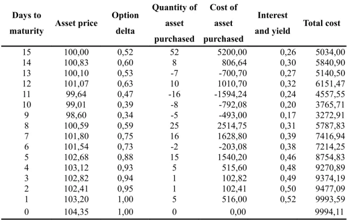
Each call option contract is on 100 units of the underlying asset. Disregard weekends and assume that the portfolio rebalancing is done once a day at the close of the market. Table 1 illustrates the delta hedging procedure for a possible sample path of the asset price.

Days to

maturity Asset price

Option delta Quantity of asset purchased Cost of asset purchased Interest

and yield Total cost

15 100,00 0,52 52 5200,00 0,26 5034,00 14 100,83 0,60 8 806,64 0,30 5840,90 13 100,10 0,53 -7 -700,70 0,27 5140,50 12 101,07 0,63 10 1010,70 0,32 6151,47 11 99,64 0,47 -16 -1594,24 0,24 4557,55 10 99,01 0,39 -8 -792,08 0,20 3765,71 9 98,60 0,34 -5 -493,00 0,17 3272,91 8 100,59 0,59 25 2514,75 0,31 5787,83 7 101,80 0,75 16 1628,80 0,39 7416,94 6 101,54 0,73 -2 -203,08 0,38 7214,25 5 102,68 0,88 15 1540,20 0,46 8754,83 4 103,12 0,93 5 515,60 0,48 9270,89 3 102,82 0,94 1 102,82 0,49 9374,19 2 102,41 0,95 1 102,41 0,50 9477,09 1 103,20 1,00 5 516,00 0,52 9993,59 0 104,35 1,00 0 0,00 9994,11

The initial Black-Scholes-Merton call option price is 1,66 and the risk manager receives 1,66 x 100 = 166 upfront. The delta of the call is initially 0,52 so the hedger buys 52 units of the underlying asset for 100 x 52 = 5200. Total cost for first day of hedging is 5200 minus the premium received from the option buyer for a total of 5034 borrowed at the risk-free interest rate to finance the asset purchase.

On the second day the asset price has moved to 100,83 and the new option delta is 0,60. The risk manager finds himself short of 8 underlying assets and buys them in the market for 100,83 x 8 = 806,64 that he borrows. At the same time, the risk manager has incurred in interest costs from the loan he took to buy the underlying asset in day 1 and received the corresponding yield from the assets in his portfolio. The result is a total cost at the end of day 2 of 5034 + 806,64 + 0,26 = 5840,90.

Next day the asset price falls to 100,10. The risk manager has 60 underlying assets, more than the new call option delta of 0,53, and sells 7 in the market realizing 100,10 x 7 = 700,70 that he uses to payback the money he borrowed after paying interest and receiving the asset yield. His total cost for the hedge is now 5840,90 – 700,70 + 0,30 = 5140,50.

The risk manager follows this procedure every day to keep a riskless portfolio. On the expiration day, the asset price is 104,35. As the option is in-the-money, the risk manager sells all the underlying asset in his portfolio realizing 104,35 x 100 = 10435 from which he uses (104,35 – 100) x 100 = 435 to fulfil his obligation to the buyer of the option and the remainder to payback the borrowed 9994,11. His net result is a profit of 5,89.

If the risk manager followed the Black-Scholes-Merton model and rebalanced his portfolio continuously as the underlying asset evolved to the expiration date, realizing the same volatility used as input to the model, he would be guaranteed by the model that the hedging cost incurred in the portfolio rebalancing would be exactly the initial value of the option, no matter the path the asset price took, resulting in profit and loss (P&L) of zero.

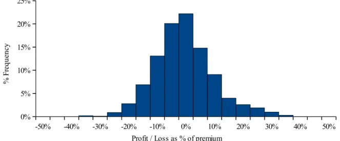
In practice it is impossible to continuously rebalance the portfolio because markets close, trading has costs, liquidity is finite and buying and selling is not always done at the desired price. The risk manager will have to choose discrete times to adjust the underlying asset position of his portfolio. As the previous example of delta hedging shows, the risk manager will end up with some P&L. In Kamal (1999) is shown that the standard deviation of the P&L, or hedging error, is directly proportional to the frequency of rebalancing but the average

result will be zero as if the hedging was carried out continuously. Figure 5 shows the P&L distribution for 1000 simulations of the delta hedging procedure for the previous call option which resulted in an average P&L around zero.

As mentioned before, the gamma of an option measures the change in delta as the underlying asset moves. As hedging cannot be carried out continuously, the gamma of the option will play a crucial role in the final P&L of the delta hedging strategy. When the absolute value of gamma is high, the risk manager will make a higher profit if long gamma and a higher loss if short gamma when the portfolio is rebalanced because the delta that needs to be adjusted is higher.

One of the inputs of the Black-Scholes-Merton model is the volatility and the model assumes that volatility is constant. In practice, volatility is seldom constant. Unlike the remaining parameters, with the exception of the asset yield that might be uncertain, volatility cannot be directly observed in the market. We can only calculate the asset return volatility realized over a period of time at the end of that time, therefore, volatility has to be estimated. The risk manager should note that the delta hedging procedure assumes that one can correctly estimate the underlying asset future realized volatility over the life of the option.

In standard call and put options, if one sells an option with implied volatility lower than the future realized volatility, a loss will be incurred as selling the option translates into a short volatility position. If an option is sold with implied volatility greater than the future realized volatility, then a gain will be made.

Figure 5: Profit and loss distribution of 1000 simulations of the delta hedging procedure.

-50% -40% -30% -20% -10% 0% 10% 20% 30% 40% 50% 0% 5% 10% 15% 20% 25%

Profit / Loss as % of premium

% F re qu en cy

The explanation is that the premium of an option is the amount the buyer of the option pays the seller to cover the expected loss made in the delta hedging procedure. If an option is sold with greater implied volatility than the future asset return volatility, the seller of the option will not lose as much money as the premium received because the expected adjustments to the replication portfolio are smaller, resulting in an expected positive difference.

When we are dealing with barrier options this behaviour is not so simple because, as we have seen before, a barrier option can have positive and negative vega over its life. If we have sold the barrier option and at a specific time the option vega is positive, money will be made if the underlying asset volatility rises. On the contrary, if vega becomes negative, the rise in volatility will lead to a loss.

3.2 Put-Call Symmetry

The put-call symmetry is a relationship between calls and puts with different strikes first studied by Bates (1988). It can be viewed as both an extension and a restriction on the put-call parity relationship between calls and puts of the same strike. Under the assumptions of the Black-Scholes-Merton model and further enforcing the drift rate of the underlying asset to be zero, the following relationship holds

C  K₁



P  K₂



where the geometric mean of the call strike K1 and the put strike K2 is the forward price F



The zero drift assumption implies that the forward price must be equal to the spot price thus requiring zero carrying cost for options written on the spot price of the underlying asset.

This relationship can be shown to hold with restrictions even if we relax the Black-Scholes-Merton model assumption that the volatility of the asset is a known constant. Carr (1998) shows that if the volatility of the forward price F is a known function of time σ(Ft, t) of the

 Ft, t=  F2/Ft, t ∀Ft≥0∧t ∈[0, T ] (68)

This means that the volatility of the forward price F at any future date is the same for any two levels with the same geometric mean thus providing support for a symmetric volatility smile. As an example consider an asset whose current forward price is 100 and the volatility is 20%. The value of a call option on the asset with strike price 125 and volatility 25% is the same as the value of 1,25 put options with strike 80 as long as the volatility at this strike is also 25%. In Carr (1994) the authors are able to use this symmetry to create a static replication portfolio for barrier options. Given the previous assumptions, the sale of a down-and-in call option when the strike K and the barrier H are equal is hedged by buying a standard put option with strike K. If the barrier is touched, put-call parity implies that, when the asset drift rate is zero, the value of the put option is equal to the value of one call option with the same strike and maturity. One can then sell the put option bought and use the proceeds to buy the call option that knocks-in without any out of pocket expenses. If the barrier is never breached the put options expire worthless as does the down-and-in call.

When the barrier H is below the strike K and the barrier is breached we need to buy an out-of-the-money call option. In this case the put in the replication portfolio is at-out-of-the-money which translates into very different values between this put option and the emerging call option. Nevertheless the same hedging strategy can be used provided that we replace the put-call parity with the put-call symmetry. The relationship ensures that by going long K/H puts with strike H2_{/K we will have the funds needed to buy the call option with strike K if the barrier is} touched. On the other hand, the puts, as the down-and-in call, will expire worthless if the barrier is not touched.

If the barrier H is above the strike K the hedging strategy has to be different because the emerging call is in-the-money and thus has intrinsic value. Define a down-and-in bond as a security that pays one monetary unit if at any time until maturity the asset price is equal to or below the strike K. We can construct a replication portfolio for the down-and-in call by buying (H − K) down-and-in bonds with strike H that provide the intrinsic value of the emerging call at the barrier and a standard put option with strike K that provides the time value.

options are valued in Rubinstein (1991b). An European binary cash-or-nothing put option pays one unit of cash if the spot is below the strike at maturity. Its present value is given by

BP=e−rT_{N −x}

1



It can also be valued and statically hedged as a portfolio constructed by a large number of long standard put options struck just above the strike and short the same number of standard puts below the strike as follows

BP  K = lim n ∞ n 2

[









]

where P(K) is a standard put with strike K and BP(K) is an European binary cash-or-nothing put option with strike K.

Given that when the forward is at the barrier each binary put has approximately 50% probability to finish in-the-money when discounting the positive skew of the price distribution, it can be shown that the value of a down-and-in bond with strike K is given by

B_diK =2BP K −1

K P  K  (71)

The down-and-out call is constructed by buying a standard call option with strike K and selling the portfolio of the down-and-in call as stated by relationship (18).

We have seen that, when the barrier is below the strike, the value of an up-and-in call is equal to the value of a standard call option and, consequently, a short position in the up-and-in call is hedged by going long a standard call option. When the barrier is above the strike, the emerging call is in-the-money and the static hedging strategy has to be split, as in the down-an-in call, into a replication of the intrinsic value and time value.

Since we are in the presence of an up barrier, we need to introduce the up-and-in bond with strike K as a security that pays one monetary unit if at any time until maturity the asset price is equal to or above the strike K. The up-and-in bond value is given by

B_uiK =2BC K  1

where C(K) is a standard call with strike K and BC(K) is an European binary cash-or-nothing call with present value given by

BC=e−rT

N  x1−



As with the European binary cash-or-nothing put, the European binary cash-or-nothing call can be statically hedged with the following portfolio of standard calls

BC  K = lim n ∞ n 2

[









]

The up-and-in call can be hedged with (H − K) up-and-in bonds that provide the intrinsic value of the emerging call at the barrier. One could think that a long position in put options would provide the time value as in the replication of the down-and-in call but this could lead to problems at expiration if the put finishes in-the-money instead of out-of-the-money. The elegant solution is to go long an up-and-in put as this security can only have value at expiration if the barrier is touched and, at that moment, it will be instantly sold. To hedge the up-and-in put we can follow the same reasoning used for the down-and-in call to see that, when the barrier H is higher then the strike K, the put-call symmetry guarantees that the value of the emerging put option is the same as the value of K/H calls struck at H2_/K.

With similar reasoning we can find the replication portfolio of the remaining barrier options. Table 2 is a summary of the hedging strategy provided by the put-call symmetry when the rebate is zero, where C(X) is a call with strike X, P(X) is a put with strike X, Bui(X) is an

up-and-in bond with strike X and Bdi(X) is a down-and-in bond with strike X. When the rebate is

not zero one can use the in bonds developed to statically hedge its risk.

As mentioned before, the put-call symmetry implies that the drift rate of the asset is zero. If this is not the case than the value of the replication portfolio is no longer ensured to be zero along the barrier, in case of knock-out options, or equal to the funds required to buy the emerging option, in case of knock-in options. The reason is that the forward value at the barrier is different from the spot which implies that call and put values with the same geometric mean are no longer equal. Even so, Carr (1994) is able to deduce tight bounds for barrier option values with static hedges when the zero drift assumption is relaxed.

Option Replication Down-and-in call cdi=

{





{





{





{





{





{





{





{





Table 2: Put-call symmetry hedging strategy for barrier options with zero rebate.

As this technique uses options to build a replication portfolio instead of dealing directly with the underlying asset, the portfolio is also somewhat protected against moves in the implied volatility of the options used in the portfolio. As long as the volatility at two levels with the same geometric mean is the same, the portfolio will always match the barrier option. This means that positive and negative shifts in the skew and in the term structure of volatility do

not impact the replication portfolio value at the barrier.

3.3 Boundary Replication

In Derman (1994) a technique of static hedging using standard options as building blocks is explained. Given a particular target option, the authors are able to construct a portfolio of vanilla options with fixed weights that will replicate the target option value for a range of future times and market levels without further adjustments and within the Black-Scholes-Merton framework.

In the model, an option can be hedged with a position in the underlying asset and its theoretical value is the discounted expected payoff at the option maturity. This payoff is subject to the predefined boundary conditions of the option. If we are able to construct a portfolio of standard options that has the same value everywhere in the boundary and the same cash flows within the boundary, the model guarantees that the replication portfolio and the target option will have the same value everywhere inside the boundary.

The principle of static replication states that it is possible to replicate a target option for all future underlying asset prices and times within some boundary by constructing a portfolio of standard options with the same net cash flows within this boundary and the same values on the boundary.

To illustrate the procedure, Figure 6 shows an example of a target option with an upper

Figure 6: Boundary conditions of a general option.

A ss et p ri ce Time to expiration t=0 t=1 t=2 t=3 t=T S U_exp L_exp U₃ L₃ U₂ L₂ L₁ L₀ U₁ U₀

boundary, a lower boundary and an expiration boundary for which we try to construct a replication portfolio with standard options. The first step is to replicate the expiration boundary t=T by matching it with a combination of options with different strikes that expire at this maturity. Moving back one time step to t=3, we compute the theoretical value at this time of the options used to match the expiration boundary condition in the upper and lower boundary, which will probably be different than the theoretical value of the target option. Then we choose a new combination of standard options that, when added to the existing replication portfolio, will match the theoretical value of the target option. For the upper boundary, we enter into a position on call options with expiration date on t=T and exercise price Uexp or more. The new calls will expire out-of-the-money below asset price Uexp and not alter the payoff already achieved for that time step. The same reasoning leads to a position on put options with maturity t=T and exercise price Lexp or lower.

Having achieved the desired payoff for time steps t=T and t=3, we move back to t=2 and add more call options with expiration t=3 and strikes above U3 and put options with strike below L3. And so on until we reach time step t=0.

The more points in time that we match the target option, the better replication we can achieve. If an infinite number of matching point were used then the replication would be perfect.

It is important to note that, if the asset price hits the boundary, the replication portfolio needs to be unwound and replaced with the security that produces the target option value on expiration.

We can use the method to replicate barrier options. Consider the following up-and-out call option:

Asset price – 100 Exercise price – 100 Barrier – 120

Time to expiration – 1 year Risk-free interest rate – 5% Asset yield – 3%

Volatility – 20% Rebate – 0

The up-and-out call is a regular call option if the barrier is never breached until maturity. This is the expiration boundary condition and can be replicated by buying a standard call option with exercise price 100 and time to expiration 1 year.

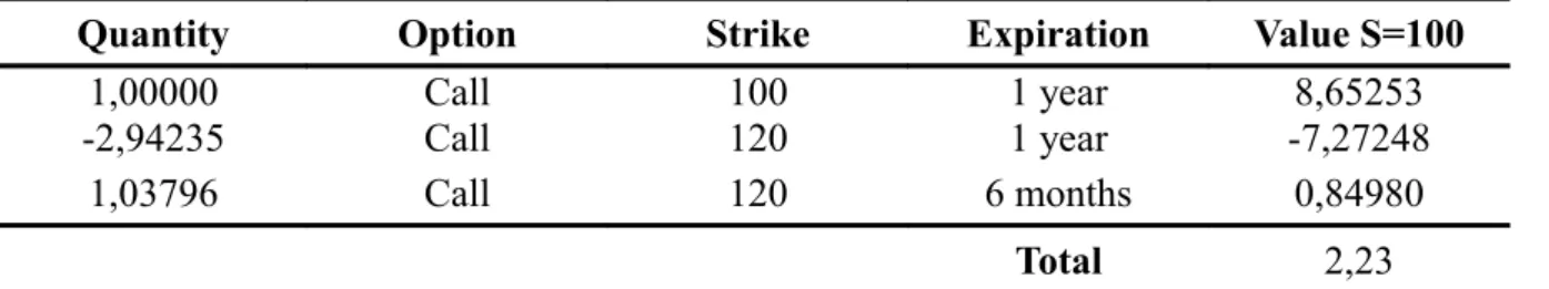
Moving back 6 months the value of this option when the asset price is at the barrier is 21,29, much higher than the theoretical value of the up-and-out call at this boundary which is zero. The solution is to eliminate this value by selling 2,94235 vanilla call options with strike 120 and one year to maturity. The quantity 2,94235 is the number of call options with strike 120 that, when the asset price is 120 and the time remaining to maturity is 6 months are valued at 7,24 each, are needed to eliminate the portfolio value of 21,29 created by the call option with strike 100. The call options sold will not alter the portfolio value already achieved for the expiration boundary because they will expire out-of-the-money inside the boundary. The sum of the values of the call options sold and the call already in the replication portfolio is now zero when we are 6 months away from maturity.

At the inception of the up-and-out call, the previous replication portfolio has a negative value of -7,51 which is lower than the up-and-out call value of zero at the barrier. To achieve the theoretical value of zero we buy 1,03796 call options struck at 120 and time to maturity 6 months so that we do not alter the replication already achieved for the final 6 months of the option life. The value of such an option is 7,24 and thus 1,03796 options are needed to void the 7,51 portfolio value.

The complete replication portfolio is given in Table 3.

Quantity Option Strike Expiration Value S=100

1,00000 Call 100 1 year 8,65253

-2,94235 Call 120 1 year -7,27248

1,03796 Call 120 6 months 0,84980

Total 2,23

Table 3: Replication portfolio of the up-and-out call with matching every 6 months.

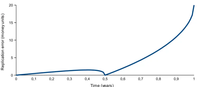
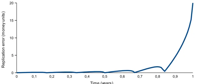
Notice that at inception the replication portfolio value is 2,23, much higher than the theoretical value of the up-and-out call option which is 1,11. Also, the portfolio suffers from substantial replication error as can be seen in Figure 7 that charts the difference between the replication portfolio value and the theoretical up-and-out call value along the barrier.

We can minimize the replication error by modelling the barrier boundary at more discrete times. Table 4 shows the replication portfolio when the boundary condition is modelled every two months. The replication portfolio value at inception is now 1,49, much closer to the 1,11 theoretical value, and the replication error is also minimized as can be seen in Figure 8.

Quantity Option Strike Expiration Value S=100

1,00000 Call 100 1 year 8,65253 -4,96280 Call 120 1 year -12,26631 2,04107 Call 120 10 months 3,90234 0,65318 Call 120 8 months 0,88475 0,30681 Call 120 6 months 0,25119 0,17626 Call 120 4 months 0,06135 0,11444 Call 120 2 months 0,00508 Total 1,49

Table 4: Replication portfolio of the up-and-out call with matching every 2 months.

If we model the barrier boundary every month, the difference between the replication portfolio value at inception and the theoretical up-and-out call value is even further minimized as shown in Table 5. At inception the value of the replication portfolio is 1,30, higher than the 1,11 theoretical value of the up-and-out call.

Figure 7: Up-and-out call replication error along the barrier, in money units, with matching every 6 months. 0 0,1 0,2 0,3 0,4 0,5 0,6 0,7 0,8 0,9 1 0 5 10 15 20 Time (years) R e p lic a tio n e rr o r (m o n e y u n its )

Quantity Option Strike Expiration Value S=100 1,00000 Call 100 1 year 8,65253 -7,04591 Call 120 1 year -17,41505 2,97941 Call 120 11 months 6,53146 1,00695 Call 120 10 months 1,92520 0,49120 Call 120 9 months 0,80168 0,28843 Call 120 8 months 0,39069 0,18953 Call 120 7 months 0,20508 0,13425 Call 120 6 months 0,10991 0,10030 Call 120 5 months 0,05725 0,07797 Call 120 4 months 0,02714 0,06249 Call 120 3 months 0,01034 0,05131 Call 120 2 months 0,00228 0,04296 Call 120 1 month 0,00007 Total 1,30

Table 5: Replication portfolio of the up-and-out call with matching every month.

Matching 2 months 1 month 2 weeks 1 week Theoretical

Value 1,49 1,30 1,20 1,15 1,11

Table 6: Comparison of the replication portfolio value with different matching intervals with the theoretical up-and-out call value.

Table 6 shows how quickly the replication portfolio value approaches the theoretical option value as the boundary matching interval is minimized. Using 26 options to match the

Figure 8: Up-and-out call replication error along the barrier, in money units, with matching every 2 months. 0 0,1 0,2 0,3 0,4 0,5 0,6 0,7 0,8 0,9 1 0 5 10 15 20 Time (years) R e p lic a tio n e rr o r (m o n e y u n its )

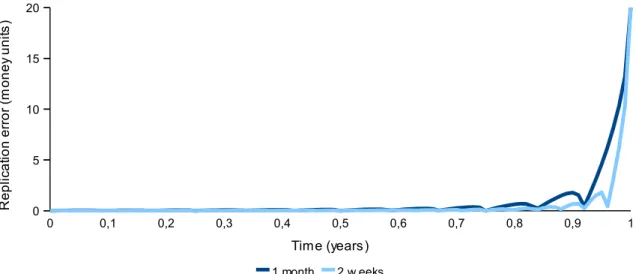
boundary the present value of the portfolio is 1,20. With 52 different options the value is 1,15. Figure 9 shows the replication portfolio error along the barrier boundary when the up-and-out call value is matched every month and every two weeks. It can be seen that the biggest problem is modelling the target barrier option close to expiration.

If at any time the barrier is hit, the portfolio is unwound and the theoretical value of zero should be realized. In practice, the value of the replication error along the barrier, which in this case is always positive, will be realized resulting in a profit to the risk manager.

Now consider an up-and-in call option with the same characteristics as the up-and-out. The up-and-in option is worth nothing at the expiration if the barrier is never breached so the replication of the expiration boundary is any empty portfolio. Working back one month we have a theoretical value of zero for the replication portfolio because there are no options in it while we should have the theoretical value of 20,12 that corresponds to the value of a call option with strike 100 and maturity in 1 month. To match the boundary value we add call options with time to expiration 1 year and strike 120 until their value at that time is 20,12. We go back another month and repeat the process until we reach the initial time and have a complete replication portfolio.

We can also recall equation (19) which states that an up-and-in call is the same as buying a standard call option and selling an up-and-out call to see that the replication portfolio shown in Table 7 is just the inverse position in the options of Table 5 without buying the call with

Figure 9: Up-and-out call replication error along the barrier, in money units, with matching every month and every two weeks.

0 0,1 0,2 0,3 0,4 0,5 0,6 0,7 0,8 0,9 1 0 5 10 15 20 1 month 2 w eeks Time (years) R e p lic a tio n e rr o r (m o n e y u n its )

strike 100 used to match the expiration boundary .

Quantity Option Strike Expiration Value S=100

7,04591 Call 120 1 year 17,41505 -2,97941 Call 120 11 months -6,53146 -1,00695 Call 120 10 months -1,92520 -0,49120 Call 120 9 months -0,80168 -0,28843 Call 120 8 months -0,39069 -0,18953 Call 120 7 months -0,20508 -0,13425 Call 120 6 months -0,10991 -0,10030 Call 120 5 months -0,05725 -0,07797 Call 120 4 months -0,02714 -0,06249 Call 120 3 months -0,01034 -0,05131 Call 120 2 months 0,00228 -0,04296 Call 120 1 month -0,00007 Total 7,35

Table 7: Replication portfolio of the up-and-in call with matching every month.

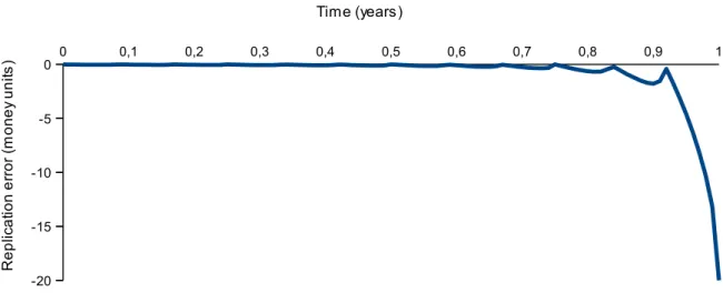
If the barrier is hit at any time until expiration the portfolio is unwound and the theoretical value needed to buy the call option with strike 100 is realized. In practice, the value realized is subject to the replication error which, in this case, is negative as shown in Figure 10. This means that the replication portfolio may not provide sufficient funds to buy the emerging option in case the barrier is breached.

Figure 10: Up-and-in call replication error along the barrier, in money units, with modelling every month. 0 0,1 0,2 0,3 0,4 0,5 0,6 0,7 0,8 0,9 1 -20 -15 -10 -5 0 Time (years) R e p lic a tio n e rr o r (m o n e y u n its )

Matching 2 months 1 month 2 weeks 1 week Theoretical

Value 7,16 7,35 7,46 7,5 7,55

Table 8: Comparison of the replication portfolio value with different matching intervals with the theoretical up-and-in call value.

Table 8 show the convergence of the replication portfolio to the theoretical option price as the number of matching times increases.

Now consider the following down-and-out call option: Asset price – 100

Exercise price – 100 Barrier – 90

Time to expiration – 1 year Risk-free interest rate – 5% Asset yield – 3%

Volatility – 20% Rebate – 0

Theoretical value – 7,08

The down-and-out call option is a regular option while the barrier is not breached so the expiration boundary is a vanilla call option with exercise price 100 and expiration in one year. The difference in the replication portfolio relative to the up-and-out call is the presence of a lower boundary which will force us to use put options with exercise price 90 or lower to match the down-and-out on the barrier. An example of a replication portfolio is shown on Table 9. The theoretical value of the portfolio at inception is 7,07, only 0,01 away from the theoretical value of the theoretical value of the down-and-out call. If the barrier is hit the portfolio is unwound for a theoretical value of zero.

Using equation (18) we can quickly find the replication portfolio for the down-and-in call by reversing the positions in the put options of Table 9 and forgetting about the call option because the expiration boundary is zero if the barrier is never touched. If, at any time until expiration, the barrier is indeed breached then the hedger ought to unwind the replication portfolio and use the realized value to buy a call option with strike 100 and expiration on the