Edilean Kleber da Silva Bejarano Aragón Marcelo Savino Portugal
Resumo
Este trabalho investiga a existência de possíveis assimetrias nos objetivos do Banco Central. Assumindo que a função perda é assimétrica em relação a desvios positivos e negativos do gap do produto e da taxa de inflação em relação à meta, nós estimamos uma função de reação não linear que permite identificar e testar a significância estatística dos parâmetros de assimetrias nas preferências da autoridade monetária. Para o período de 2000-2007, os resultados indicaram que o Banco Central brasileiro apresentou uma preferência assimétrica a favor de uma inflação acima da meta. Visto que este comportamento pode ser decorrente das decisões de política em momentos de fortes crises (tais como as de 2001 e 2002), nós delimitamos a nossa amostra para o período de 2004-2007. Para este período, nós não encontramos evidências empíricas apontando para qualquer tipo de assimetria nas preferências sobre a estabilização da inflação e do gap do produto.
Palavras-Chave
política monetária, preferências assimétricas, regras de taxa de juros não lineares, Brasil
Abstract
This paper investigates the existence of possible asymmetries in the Central Bank of Brazil’s objectives. By assuming that the loss function is asymmetric with regard to positive and negative deviations of the out-put gap and of the inflation rate from its target, we estimated a nonlinear reaction function which allows identifying and checking the statistical significance of asymmetric parameters in the monetary authority’s preferences. For years 2000 to 2007, results indicate that the Central Bank of Brazil showed asymmetric preference over an above-target inflation rate. Given that this behavior may stem from policy decisions in periods of severe crises (e.g., in 2001 and in 2002), we restricted our sample to the 2004-2007 period. We did not find any empirical evidence of any type of asymmetry in the preferences over the stabilization of inflation and of the output gap for this period.
Keywords
monetary policy, asymmetric preferences, nonlinear interest rate rules, Brazil
JEL Classiication E52, E58
The authors would like to thank the comments of two anonymous referees that helped to improve the article.
Department of Economics, Universidade Federal da Paraíba (UFPB). E-mail: [email protected].
Department of Economics, Universidade Federal do Rio Grande do Sul (UFRGS) and CNPq. E-mail:
Contact address: Universidade Federal da Paraíba – CCSA – Departamento de Economia – Cid. Universitária – João Pessoa – PB – Brasil. CEP: 58059-900.
1 Introduction
Ever since the early 1990s the economic literature dealing with the analysis of monetary policy actions by way of reaction function estimates has been gaining mo-mentum. Taylor (1993) rule is probably the most widely known specification of this reaction function in this literature. According to this rule, the monetary authority responds to deviations of output and of inflation from their targets through nomi-nal interest rate fluctuations regarded as policy instrument. Another specification that has received considerable attention is the forward-looking reaction function proposed by Clarida et al. (1997, 2000). In this type of policy rule, the policymaker adjusts the current interest rate by considering the future values expected for infla-tion and for the output gap. A common feature of these two types of interest rate rules is that they are linear functions relative to variables that describe economic conditions. This can be explained by the fact that both specifications are theoreti-cally based upon the linear-quadratic model, where the monetary authority’s loss function is assumed to be quadratic and the equations describing the economic framework are linear.
Nevertheless, two theoretical approaches were developed recently which have challenged the linear-quadratic framework behind the linear reaction function. The first approach rejects the assumption that the economic framework is linear. Orphanides and Wieland (1999) derive optimal policy rules for the case in which the monetary authority presents a quadratic loss function and is faced up with a zone-linear Phillips curve that allows for nonlinearities in the short-term trade-off between inflation and output. Nobay and Peel (2000) assessed optimal discretio-nary monetary policy under a nonlinear Phillips curve and found that the monetary authority can no longer remove the inflation bias by establishing a target for the ou-tput that equals the natural rate. Dolado et al. (2005) demonstrate that the central bank’s optimal reaction function for an economy with a nonlinear Phillips curve is a forward-looking interest rate rule that has been increased in order to include the interaction between expected inflation and the output gap.
the policymaker’s loss function. In addition, in periods during which the monetary authority is more concerned with lending credibility to its disinflationary policy, the loss due to positive deviations of the inflation rate from its target is likely larger than that one resulting from negative deviations of the same magnitude.
The consequences of including asymmetric preferences in the monetary authority’s loss function have been investigated by several authors. Cukierman (2000) de-monstrates that when the policymaker is uncertain about the economic conditions and when he is more sensitive to negative output gaps, an inflation bias arises even when the target for the actual output is the potential output of the economy. This result has been supported by empirical evidence gathered by Cukierman and Gerlach (2003) for a group of 22 OECD (Organization for Economic Cooperation and Development) countries. Gerlach (2000) and Surico (2007) found out that the Federal Reserve was more worried about negative output gaps than about posi-tive ones in the pre-1980 period. Bec et al. (2002) verified that the business cycle phase, measured by the output gap, has played an important role in the conduct of monetary policy by the central banks of Germany, USA and France. Cukierman and Muscatelli (2003, 2008) provide evidence of nonlinearities regarding inflation and output gap in reaction functions estimated for Germany, the United Kingdom and the USA. Dolado et al. (2004) observed that Federal Reserve’s preferences regarding inflation were asymmetric during the Volcker-Greespan era.
Following this line of research, the present paper seeks to estimate a nonlinear re-action function for the Central Bank of Brazil that allows testing the existence of asymmetries in their objectives regarding inflation and output during the inflation targeting regime. Taking the model proposed by Surico (2007) as our theoretical framework, we obtain an optimal monetary policy rule for the monetary authority considering that its loss function is potentially asymmetric. Given that the presence of asymmetries in objectives produces nonlinear responses of the interest rate to inflation and to the output gap, we checked whether the policymaker’s preferences are symmetric by testing the null hypothesis of linearity of the reaction function. Also, we estimated the asymmetric parameters in the Central Bank’s preferences and tested whether these coefficients are statistically significant.
interest rate during and outside the periods of exchange rate crises. Minella et al. (2003), Holland (2005), Policano and Bueno (2006), Soares and Barbosa (2006) and Teles and Brundo (2006) showed that in the inflation targeting regime the Selic interest rate strongly reacted to expected inflation. Bueno (2005) and Lima et al. (2007) estimated a Markov-switching reaction function and found evidence of diferent monetary policy regimes after the Real Plan Real. Neto and Portugal (2007) estimated the reaction functions for the chairmanships of Armínio Fraga and Henrique Meirelles and found evidence supporting the conduct of monetary policy in the inflation targeting regime. Even though some of these studies consider nonlinearities in the reaction function, none of them seeks to confirm whether the Central Bank’s preferences regarding inflation and output have been asymmetric.
This paper is organized as follows. Section 2 lays out the theoretical model and derives the optimal reaction function for the interest rate as a first-order condition for the Central Bank’s optimization problem. Section 3 presents the reduced form for the interest rate rule to be estimated in order to check the existence of asym-metries in the monetary authority’s objectives. Section 4 shows and analyzes the results. Finally, Section 5 concludes.
2
The Theoretical Model
The present paper is theoretically based upon the model proposed by Surico (2007). The model uses the new-Keynesian structure assessed by Clarida et al. (1999) and allows the monetary authority to have asymmetric preferences with regard to its objectives or targets. Specifically, the monetary authority is allowed to be more averse to negative deviations of the actual output from the potential output and to positive deviations of the inflation rate from the inflation target. The presence of these types of asymmetries constitutes the explanation for possible nonlinear res-ponses of the monetary policy interest rate to inflation and output fluctuations.
2.1 structure of the Economy
Following Clarida et al. (1999), we considered an economy whose evolutionary behavior can be described by the following equations:
1 1
( )
t t t t t t t
x = −ϕ − πi E + +E x+ +e (1)
1
t kxt Et t+ ut
where xt is the output gap (the difference between actual output and potential
output), πt is the inflation rate, Etxt+1 and Et πt+1 are the expected values for the output gap and for inflation conditional on the information available at t, it is the
nominal interest rate, et is a demand shock, ut is a cost shock and ϕ, k and θ are
positive constants.1
The IS curve, represented by equation (1), is a log-linearized version of consumption Euler equation which is derived from the optimal family decision about consump-tion/saving, after the imposition of the market clearing condition. The expected future output gap shown in this equation indicates that, since families prefer to cut down consumption over time, the expectation for a higher level of consumption in the future leads to higher consumption in the present, thus increasing the current demand for output.
Phillips curve (2) captures the characteristic of staggered nominal prices in which each firm has a probability θ of keeping the price of its product fixed in any time period (CALVO, 1983). Given that probability θ is supposedly constant and inde-pendent of the time elapsed since the last adjustment, the average time at which the price is kept fixed is given by 1/1-θ. This discrete nature of price adjustment encourages each firm to set a higher price the higher the expected future inflation. The positive effect of the output gap on inflation reflects the increase in marginal costs produced by excess demand.
Finally, shocks et and utcomply with the following autoregressive processes:
1
t e t t
e
= ρ
e
−+
ê
(3)where 0 ≤ ρe, ρu≤ 1 and, êt and ût are i.i.d random variables with zero mean and
standard deviationsσe and σu, respectively.
1
t u t t
u
= ρ
u
−+
û
(4)where 0 ≤ ρe,ρu ≤ 1 and, êt and ût are i.i.d random variables with zero mean and
standard deviations σe and σu, respectively.
1 The aggregate behavioral equations (1) and (2) are explicitly derived from the optimizing beha-vior of firms and families in an economy with currency and nominal price rigidity (CLARIDA
2.2 Monetary authority’s asymmetric objectives
Suppose that monetary policy decisions are made before shocks et and ut. Therefore,
conditional on the information available at the end of the previous period, the mo-netary authority tries to choose current interest rate it and a sequence of future
interest rates so as to minimize:
1 0
t t
E
L
∞ τ
− +τ
τ=
δ
∑
(5)subject to equations (1) and (2), where δ is the fixed discount factor. The monetary authority’s loss function at time t, Lt, is given by:
( *) *
* 2
2 2
e 1 e ( ) 1
( )
2
t t
x
t t
t t
x
L i i
γ − γ − α π −π − α π − π − µ
= λ + + −
γ α (6)
where π*is the inflation target, λ is the relative weight on the deviation of the ou-tput gap from the potential ouou-tput and µis the relative weight on the stabilization of the interest rate. The monetary authority is assumed to stabilize inflation around the constant inflation target, π*, to maintain the output gap closed at zero and to
stabilize the nominal interest rate around its target, i*.
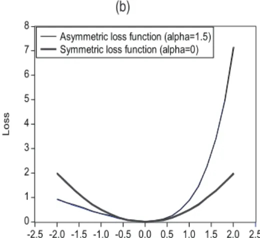
(a) (b)
Figure 1 – Symmetric and Asymmetric Loss Function Relative to Output Gap (a) and Inlation (b)
A positive value of α reveals that the monetary authority has a precautionary de-mand for price stability, i.e., the marginal loss of a positive deviation of the inflation rate from its target is larger than that of a negative deviation of the same magnitude (see Figure 1). Although this behavior is plausible, one should underscore that linex specification (6) does not prevent α from being negative, indicating that a below-target inflation rate is costlier than an above-below-target one. For the special case in whi-ch both γ and α tend towards zero, (6) is reduced to the symmetric loss function
2 * 2 * 2
1
( ) ( )
2
t t t t
L = λ + π − πx + µ −i i .
Optimization problem (5) is solved under discretion. This implies that the po-licymaker regards the expectations of future variables as given and chooses the current interest rate, reoptimizing it in each period. Since there is no endogenous persistence in inflation and in output gap, the intertemporal optimization problem can be reduced to a static optimization problem sequence. Therefore, by taking the first-order condition and solving it for it, we obtain:
( *) *
1 1 2 1
1 1
t t
x
t t t
e e
i i c E c E
γ α π −π
− −
− −
= + +
γ α
(7)
1 ; 2 k
c =λϕ c = ϕ
µ µ (8)
According to (7), the optimal nominal interest rate at time t reacts nonlinearly to inflation and to the output gap expected for time t. As c1 and c2are both positive, the monetary authority increases the nominal interest rate in response to hikes both in the expected output gap and in the expected inflation rate.
When both γ and α tend towards zero, by using the L’Hôpital’s rule, it is possible to show that equation (7) is reduced to the following reaction function:
* *
1 1 2 1
(
)
t t t t t
i
= +
i
c E x
−+
c E
−π − π
(9)In this case, the monetary policy interest rate responds linearly to the expected output gap and to the inflation rate expected for period t.2 From the comparison between equations (9) and (7), we can observe that the presence of asymmetries in the objectives of the monetary authority directly implies a nonlinear interest rate reaction function. Thus, a way to check the hypothesis of symmetric preferences is to test the functional form of the monetary authority’s reaction function.
3 Reduced-Form Reaction Function
In this section, we derive the reduced form for the interest rate rule to be estima-ted so as to check the existence of asymmetries in the Central Bank’s loss function during the inflation targeting regime. As pointed out by Surico (2007), the estima-tion procedures of the model and of the test of the null hypothesis of symmetric preferences (H0:γ=α=0) are complex due to the indeterminacy of important
para-meters and due to the presence of unidentified nuisance parapara-meters under the null hypothesis. For instance, if γ=α=0, then the coefficients related to the inflation rate and to the output gap in reaction function (7) are indeterminate. In addition, when α=0, the inflation target is an unidentified nuisance parameter, implying that the conventional statistical theory is not available for obtaining the asymptotic distribution of statistical tests under the null hypothesis (LUUKKONEN et al., 1988; VAN DIjK et al., 2002).
2 This type of implicit interest rate rule was analyzed by Rudebusch (2002) and Clarida et al.
To circumvent these problems, we followed the suggestion given by Luukkonen et al. (1988) and linearized the exponential terms in (7) by way of a first-order Taylor expansion aroundγ=0 and α=0. The result of this procedure is the following reduced-form reaction function:
* * * 2 2
1( ) 1 1( ) 1
2 2
t
t t t t t t t t t
k k
i i E− E x− E− E x−
z
ϕ λϕ α ϕ γλϕ
= + π − π + + π − π + +
µ µ µ µ µ (10)
where zt is the remainder ofthe Taylor series approximation.
In order to get to the final specification of the reaction function to be estimated in this paper, we considered two changes to equation (10). First, we introduced two interest rate lags to capture the tendency of the monetary authority towards smoo-thing the changes in the monetary policy instrument and towards avoiding serial autocorrelation problems.3 Among the possible explanations to this smoothing, we highlight the following: i) uncertainties over the data and over the coefficients in the monetary transmission mechanism; ii) the policymakers’ actions are taken only when they are confident about the results to be produced by these actions; iii) large changes in interest rates can destabilize the financial and exchange rate markets; iv) reversions in monetary policy actions may be seen as errors or evidence of policy inconsistency; v) small but persistent changes in the short-term interest rate cause a remarkable effect of the monetary policy on aggregate demand without requiring excess volatility of this interest rate.4,5
The second change consists in replacing the expected inflation and output gap va-lues in (10) with their realized vava-lues. This way, we obtain the following interest rate reaction function:
* * 2 2
1 2 0 1 2 3 4 1 1 2 2
(1 )[ ( ) ( ) ]
t t t t t t t t
i = −ρ −ρ d + π − π +d d x +d π − π +d x +ρi− +ρ i− +υ (11)
3 For Brazil, interest rate smoothing by the Central Bank was observed by Silva and Portugal (2001), Minella et al. (2003), Salgado et al. (2005), Bueno (2005) and Neto and Portugal (2007).
4 For a theoretical and empirical study of monetary policy interest rate smoothing, see Clarida et al. (1997), Sack (1998), Woodford (1999, 2003), Sack and Wieland (2000), Srour (2001). 5 Woodford (1999, 2003) demonstrated that the interest rate rule for a Central Bank which can
where the coefficients di, i=0,...,4, are given by
*
0
;
1;
2;
3;
42
2
k
k
d
=
i
d
=
ϕ
d
=
λϕ
d
=
α ϕ
d
=
γλϕ
µ
µ
µ
µ
(12)And the error term υt is defined as
{
2 2 2 2}
1 2 1 1 2 1 3 1 4 1
(1 ) ( ) ( ) [ ( ) ] [ ( ) ] t
t d t Et− t d xt E xt− t d t Et− t d xt Et− xt
z
υ = − −ρ −ρ π − π + − + π − π + − +
µ (13) From expression (13), we may observe that the term in curly brackets is a linear combination of forecast errors and, for that reason, υt is orthogonal to any variable
of the model available in the information set at t-1.
Two important characteristics of reaction function (11) should be underscored. The first concerns the fact that the hypothesis of symmetry in the monetary authority’s objectives can be tested by estimating coefficients di’s. From (11) and (12), one
can see that the imposition of restriction γ=α=0 corresponds to d3 =d4=0. Thus,
testing the null hypothesis of symmetric preferences, H0:γ=α=0, is the same as
testing the null hypothesis of linearity, H’0=d3= d4=0.6 The statistical significance
of the restrictions imposed by H’0 can be verified by the Wald test. Under H’0, the
Wald test statistic has approximately a χ2 distribution with r degrees of freedom, where r is the number of restrictions imposed. The second characteristic is that the reduced form of the monetary policy rule allows obtaining estimates for the asymmetric parameters in the loss function, since α=2d3/d1 and γ=2d4/d2.
In addition to reaction function (11), we estimated five alternative specifications in order to render the empirical model more suitable to the conduct of the Brazilian monetary policy in the current inflation targeting regime. First, we considered a deviation from the original assumption that the inflation target is constant. This modification is necessary since in the 1999-2004 period, the inflation targets, esta-blished by the National Monetary Council (NMC), changed annually.7 Therefore, the specification with a time-varying inflation target is given by:
* * 2 2
1 2 0 1 2 3 4 1 1 2 2
(1 )[ ( ) ( ) ]
t t t t t t t t t t
i = −ρ −ρ d + π − π +d d x +d π − π +d x +ρi− +ρ i− +υ (14)
6 The power of the test which is based on reaction function (11) depends on the confirmation that d1and d2 are statistically different from zero because it is possible not to reject the null
hypothesis of linearity since these coefficients are equal to zero.
In the second alternative specification, we considered that the Central Bank reacts to deviations of the expected inflation from the inflation target. By knowing that the inflation targets for year T and T+1 in the Brazilian inflation targeting regime are disclosed to the policymaker at the beginning of year T, it is plausible to as-sume that monetary policy actions are taken based on the deviation of expected inflation from the target for the current and subsequent years. Thus, we followed the suggestion given by Minella et al. (2003) and we used the variable Dj, which is a weighted measure of the deviation of the expected inflation for years T and T+1 from their respective inflation targets, i.e.:
* *
1 1
(12 )
( ) ( ).
12 j T T 12 j T T
t
Dj = − j Eπ − π + j Eπ + − π + (15)
where j is the monthly rate, EjπT is the inflation expectation in month j for year T,
EjπT+1 is the inflation expectation in month j for year T+1, π*T is the inflation target
for year T and π*
T+1 is the inflation target for year T+1. The nonlinear reaction
func-tion with the variable Dj is denoted by:
2 2
1 2 0 1 2 3 4 1 1 2 2
(1 )[ ]
t t t t t t t t
i = −ρ −ρ d +d Dj +d x +d Dj +d x +ρi− +ρ i− +υ (16) Finally, we considered nonlinear reaction functions in which the interest rate reacts to the output gap at t-2 and to the deviation of inflation from its target at t-1. This assumption is justified by the fact that the monthly data on inflation and economic activity are only available to the monetary authority with a lag of 1 and 2 periods, respectively. Therefore, we estimated the following specifications:
* * 2 2
1 2 0 1 1 2 2 3 1 4 2 1 1 2 2
(1 )[ ( ) ( ) ]
t t t t t t t t
i = −ρ −ρ d + π − π +d − d x− + π − π +d − d x− +ρ i− +ρ i− +υ (17)
* * 2 2
1 2 0 1 1 1 2 2 3 1 1 4 2 1 1 2 2
(1 )[ ( ) ( ) ]
t t t t t t t t t t
i = −ρ −ρ d + π − π +d − − d x− + π − πd − − +d x− +ρi− +ρ i− +υ (18)
2 2
1 2 0 1 2 2 3 4 2 1 1 2 2
(1 )[ ]
t t t t t t t t
i = −ρ −ρ d +d Dj +d x− +d Dj +d x− +ρi− +ρ i− +υ (19)
4 Results
4.1 Data Description
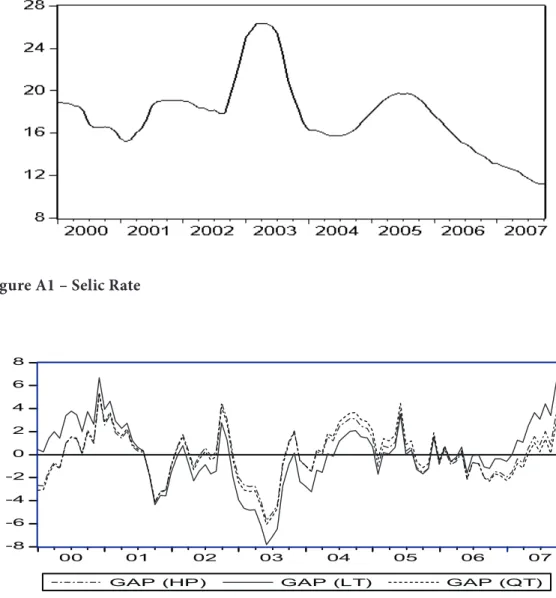
October 2007. The series were obtained from the Institute for Applied Economic Research (IPEA) and from the Central Bank of Brazil websites.8 The dependent variable, it, is the annualized monthly Selic interest rate. This variable has been used
as the major monetary policy instrument in the inflation targeting regime.
The inflation rate, πt, is the inflation accumulated in the past 12 months, measured
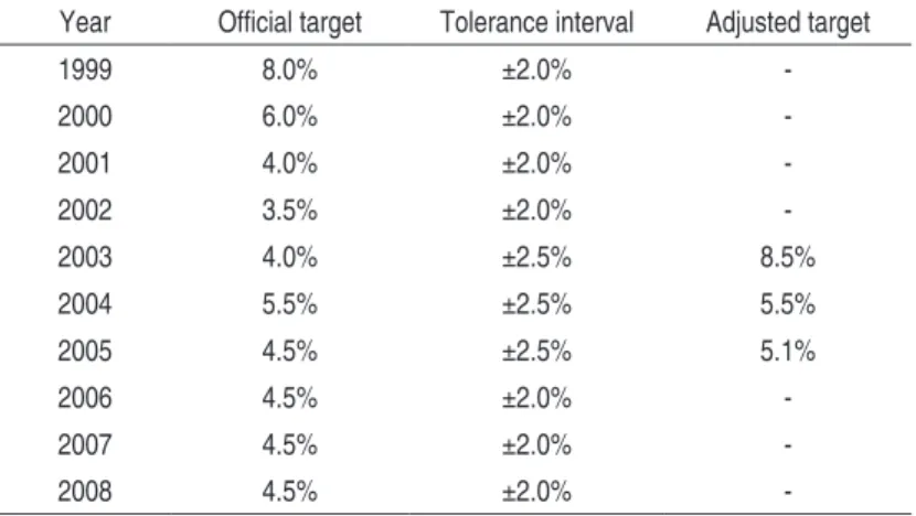
by the Broad Consumer Price Index (IPCA).9 For the specification that includes the deviation of inflation from a constant target, we used the mean annual inflation targets. 10 Where inflation targets were time-varying, we interpolated the annual targets in order to obtain the series with monthly frequency.11
The variable Djtpresent in specifications (16) and (19) is built from inflation
tar-gets established for years T and T+1, and from the series of inflation expectations obtained from the survey conducted by the Central Bank at financial institutions and consultancy firms. In this survey, firms are supposed to state the inflation rate they expect for years T (EjπT) and T+1 (EjπT+1).
The output gap (xt) is measured by the percentage difference between the
seaso-nally adjusted industrial production index (yt) and the potential output (ypt), i.e.,
xt = 100(yt- ypt)/ypt. Here, there is an important problem due to the fact that the
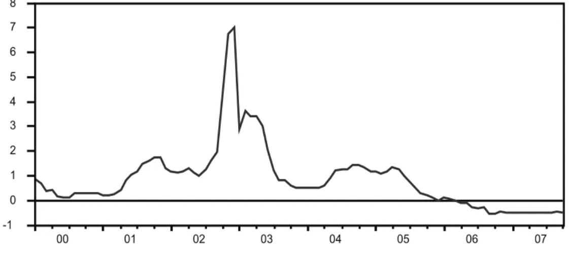
potential output is an unobserved variable and, for that reason, should be estimated. Thus, we obtained the proxy variable for the potential output in three different ways: using the Hodrick-Prescott (HP) filter, using a linear trend (LT) and using a quadratic trend (QT). The output gap series constructed from different potential output estimates are called x1t (HP), x2t (LT) and x3t (QT). Finally, we added the
dummy variable Di,t (=1 for 2002:10-2003:02 and 0, otherwise) in all specifications
of the reaction function so as to capture the quick and strong increase in the Selic rate that resulted from the rise in inflation and in inflation expectations at the end of 2002 and at the beginning of 2003.
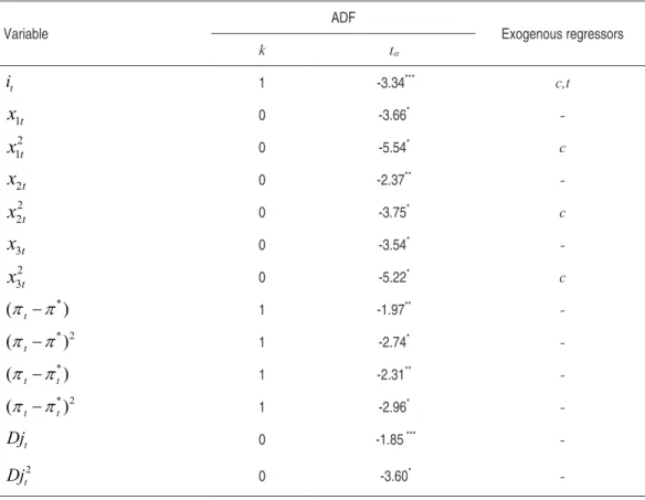
Before estimating the reaction function, we ran ADF tests to check the stationarity of the model’s variables. We chose the optimal number of lagged difference terms to be included in each regression, k, based on the Schwarz information criterion. The maximum autoregressive order was equal to 24. For the squares of the three
8 The graphs for the series used are shown in the Appendix A.
9 The IPCA is calculated by the Brazilian Institute of Geography and Statistics (IBGE) and is the price index used by the NMC as benchmark for the inflation targeting regime.
10 In all years, except for 2003, we used the central inflation targets as determined by the NMC. In 2003, the target used was the one adjusted by the Central Bank (8.5%).
11 To obtain the inflation target for the past 12 months, we interpolated the annual targets using equation π*
j = [(12-j)/12]π*a,t-1 +(j/12)π*a,t, where π*j is the inflation target in month j for the past 12 months, π*
a,t-1 is the inflation target for year t-1, π*a,t is the inflation target for year t. The
output gap series, the tests included a constant (c), whereas a linear trend (t) was also included for the Selic rate.
Table 1 shows that the ADF tests reject, at a 10% significance level, the null hy-potheses that the explanatory variables in nonlinear reaction functions are not stationary.
Table 1 – Unit Root Test - ADF: 2000:01-2007:10
Variable
ADF
Exogenous regressors
k tα
t
i 1 -3.34*** c,t
1t
x
0 -3.66*-2 1t
x
0 -5.54* c2t
x
0 -2.37**-2 2t
x
0 -3.75* c3t
x
0 -3.54*-2 3t
x
0 -5.22* c*
(π − πt ) 1 -1.97**
-* 2
(π − πt ) 1 -2.74*
-*
(π − πt t) 1 -2.31**
-* 2
(π − πt t) 1 -2.96*
-t
Dj 0 -1.85 ***
-2
t
Dj 0 -3.60*
-Note: * Significant at 1%. ** Significant at 5%. *** Significant at 10%.
4.2 Estimated reaction Functions
dummy variable Di,t. These instruments imply 14 overidentifying restrictions. We
tested the validity of these restrictions by way of Hansen’s (1982) J test.
The estimation results are shown in Table 2. Specifications (A), (B) and (C) refer, respectively, to specifications with a constant inflation target, with the variable in-flation rate and with deviation of the expected inin-flation from the inin-flation target. On the other hand, specifications HP, LT and QT are related to the use of three different output gap series (x1t, x2t e x3t) as explained in section 4.1.
Right away, we may note that the estimates for parameter d3, which measures
the response of the Selic rate to the squared deviation of current inflation (or of the expected inflation) from the target, had a negative sign and were statistically significant in all of the estimated reaction functions. It should be highlighted that a negative coefficient over
π − π
t *t indicates that a reduction in the Selic rate inresponse to a decrease in inflation relative to the target of a given size is larger than the increase of this interest rate caused by an increase in the deviation of inflation with the same magnitude. This behavior is consistent with a Central Bank that has an asymmetric preference that favors an above-target inflation rate.
Due to the nonlinear framework, the responses of the monetary policy instrument to deviations of the current inflation and of the expected inflation from the infla-tion target are given by:12
*
1 3
*
2
(
)
(
)
i
d
d E
∂
= +
π − π
∂ π − π
(20)1
2
3(
)
i
d
d E Dj
Dj
∂
= +
∂
(21)where E(∙) indicates the sample mean. Using these expressions and the coefficient values shown in Table 2, we estimated that the response of the Selic rate to the deviation of inflation from its target was on average equal to 1.52 in specifications A and B, and 3.86 in specification C. This indicates that nonlinear interest rate rules satisfy Taylor’s (1993) principle. In addition, the stronger reaction of the moneta-ry policy to the expected inflation concurs with the results obtained by Holland (2005) and Soares and Barbosa (2006) and underscores the forward-looking nature of Central Bank’s decisions.
12 As variables πt-π* or Djtalso have secondary effects on the Selic rate due to inertial terms it-1 and it-2, we derived the responses of this policy instrument in the long run (it=it-1=it-2), when
be
r da s
ilva b eja ra n o a ra gó n, M ar ce lo s av in o P or tu ga l 387 E st. e co n., S ã o P au lo
, 40(2): 373-399, a
br .-j u n. 2010 Parameters Speciications
(A) (B) (C)
HP LT QT HP LT QT HP LT QT
0
d 15.25
* (0.47) 15.45* (0.42) 15.01* (0.55) 14.67* (0.59) 15.28* (0.44) 14.49* (0.58) 14.03* (0.27) 13.85* (0.45) 13.95* (0.28) 1
d 1.980*
(0.36) 1.763* (0.35) 1.985* (0.38) 2.301* (0.53) 1.841* (0.42) 2.366* (0.55) 4.244* (0.29) 4.509* (0.49) 4.300* (0.32) 2
d -0.094n.s
(0.29) -0.401** (0.17) 0.108n.s (0.35) -0.036n.s (0.42) -0.293n.s (0.21) -0.041n.s (0.40) -0.214n.s (0.16) 0.017n.s (0.13) -0.186n.s (0.15) 3
d -0.240*
(0.06) -0.251* (0.06) -0.252* (0.06) -0.271* (0.08) -0.188* (0.05) -0.270* (0.08) -0.551* (0.05) -0.588* (0.08) -0.555* (0.05) 4
d 0.109n.s
(0.09) 0.069n.s (0.05) 0.180n.s (0.11) 0.125n.s (0.10) -0.048n.s (0.08) 0.128n.s (0.09) -0.000n.s (0.04) 0.033n.s (0.03) 0.012n.s (0.04) ρ1 1.483* (0.04) 1.348* (0.06) 1.503* (0.04) 1.578* (0.07) 1.654* (0.06) 1.588* (0.06) 1.286* (0.08) 1.241* (0.08) 1.265* (0.09)
ρ2 -0.573
* (0.04) -0.460* (0.05) -0.579* (0.04) -0.689* (0.05) -0.774* (0.05) -0.694* (0.05) -0.453* (0.06) -0.429* (0.06) -0.438* (0.06)
Dummy 24.90
* (7.03) 8.544** (6.24) 26.40* (7.54) 21.80* (6.66) 17.31* (5.93) 20.54* (5.85) 8.117* (2.31) 6.690* (1.90) 7.665* (2.29)
R2 – adjusted 0.978 0.968 0.982 0.968 0.977 0.973 0.990 0.988 0.990
W(2) - prob 0.000 0.001 0.000 0.002 0.000 0.001 0.000 0.000 0.000
J(14) - prob 0.844 0.873 0.814 0.736 0.648 0.742 0.809 0.850 0.836
In general, the reaction of the interest rate at the output gap level, measured by parameter d2, was nonsignificant. The coefficient over the squared output gap, d4, was not statistically different from zero in any of the estimated models. This means that there is no empirical evidence of a nonlinear response of the monetary policy instrument to the output gap.
The last two lines in Table 2 show the p-values (prob) for the joint hypothesis of symmetric preferences and for the hypothesis of validity of overidentifying restric-tions. For all estimated specifications, the hypothesis of a linear reaction function is strongly rejected. This evidence clearly results from the nonlinear reaction of the monetary authority to the deviations of inflation from the target. The results of the J test indicate that the overidentifying restrictions cannot be rejected at a significance level of 10%.
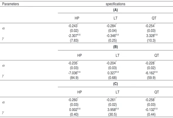
Table 3 shows the estimates for the monetary authority’s parameters of asymmetric preference. The coefficients were found using expressions α=2d3/d1 and γ=2d4/d2.
The standard errors were calculated using the delta method. Consistently with the results shown in Table 2, we can observe that the coefficients that measure the asymmetry in the preferences over the output gap, γ, were not statistically diffe-rent from zero. Conversely, the values for the asymmetric parameter regarding the preference over inflation, α, had a negative sign and were statistically significant in all estimated specifications. This indicates that the negative deviations of inflation from the target of a given size cause a greater loss for the Brazilian monetary au-thority than the positive deviations with the same magnitude.13
13 As suggested by an anonymous referee, we estimated reaction functions (11), (14) and (16)
in-cluding three lags of the variables ∆qt=qt-qt-1 and ∆12qt=qt-qt-12, where qt is the nominal exchange
Table 3 – Estimates for Asymmetric Preferences
Parameters speciications
(A)
HP LT QT
α -0.243*
(0.02)
-0.284* (0.04)
-0.254* (0.03)
γ -2.307(7.83)n.s -0.346(0.25)n.s 3.328(10.3)n.s
(B)
HP LT QT
α -0.235*
(0.03)
-0.204* (0.03)
-0.228* (0.02)
γ -7.036n.s
(84.9)
0.327n.s (0.68)
-6.162n.s (59.9) (C)
HP LT QT
α -0.260*
(0.03)
-0.261* (0.02)
-0.258* (0.03)
γ 0.002n.s
(0.40)
3.958n.s (30.5)
-0.132n.s (0.44)
Note: * Significant at 1%. n.s Nonsignificant.
In Table 4, we provide the estimates for reaction functions (17)-(19), in which the monetary policy instrument depends on the deviation of inflation from the target at time t-1 and of the output gap at time t-2. Initially, we estimated the monetary policy rules using ordinary least squares. As the ARCH test revealed remarkable problems with autoregressive conditional heteroskedasticity, we estimated the re-action functions assuming that the conditional variance of error terms follows an ARMA(p,q) process, where p is the order of the ARCH terms and q is the order of the GARCH terms. The last line in Table 4 shows the orders p and q of the GARCH models estimated by maximum likelihood.14
In general, the results are similar to those shown in Tables 2 and 3. The main diffe-rence concerns the positive and statistically significant response of the Selic rate to the output gap, measured by coefficient d2. This suggests that the measure of the economic activity entering the reaction function is the gap of the period known by the Central Bank at the time when monetary policy decisions are made. With regard to the Brazilian monetary authority’s loss function, Table 4 shows that the asymmetric parameter in the preferences over the output gap, γ, is not statistically
different from zero, whereas the coefficient that measures the asymmetry in the preferences over the deviations of inflation from the target, α, is negative and sig-nificant in eight out of nine specifications.
In brief, the set of empirical results shown above provides evidence that the Central Bank of Brazil has been more averse a to below-target inflation than to an above-tar-get one. This behavior is the opposite of the one expected by a monetary authority that is more concerned with lending credibility to its disinflationary policy. A pos-sible explanation to this is that the concavity of the reaction function with regard to deviations of the inflation rate from the target may reflect the monetary policy decisions made in periods of supply shocks (such as the energy crisis in 2001) and of fiscal dominance (last quarter of 2002).15 On any of these occasions, the Central Bank might have adopted a more gradualist behavior toward inflation control than that which is expected from a policymaker with asymmetric preference over a target inflation. Also, the Brazilian experience with inflation the below-central target is recent and relatively short. For instance, when one considered the inflation deviation series compared to a variable target, only 30 of 94 observations showed values smaller than zero. On the other hand, for inflation deviation series with a fixed target, πt-π*, and deviation of the expected inflation from the target,
Djt, the number of observations with negative values drops to 19.
Based on this, we decided to estimate nonlinear reaction functions for the period between january 2004 and October 2007. The advantages of using this period are the greater stability of the economic activity, lower predominance of shocks affec-ting inflation expectations and a larger balance between the number of observations in which inflation was above and below target.
be
r da s
ilva b eja ra n o a ra gó n, M ar ce lo s av in o P or tu ga l 391 E st. e co n., S ã o P au lo
, 40(2): 373-399, a
br
.-j
u
n. 2010
Parameters (A) (B) (C)
HP LT QT HP LT QT HP LT QT
0
d 15.17*
(0.26) 15.37* (0.23) 14.89* (0.36) 15.24* (0.60) 14.79* (0.91) 14.95* (0.62) 14.47* (0.52) 13.85* (0.76) 14.34* (0.50) 1
d 1.397*
(0.15) 1.493* (0.16) 1.313* (0.18) 0.932* (0.33) 1.571* (0.44) 0.934* (0.32) 4.286* (0.84) 6.170* (1.23) 4.042* (0.74) 2
d 0.441**
(0.18) 0.353
**
(0.18) 0.431
**
(0.19) 1.081
*
(0.34) 0.758
***
(0.41) 0.975
*
(0.29) 1.070
*
(0.41) 1.049
**
(0.45) 0.938
*
(0.30)
3
d -0.096*
(0.03) -0.098 * (0.03) -0.099 * (0.04) -0.077 n.s (0.05) -0.142 ** (0.07) -0.064 n.s (0.05) -0.721 * (0.20) -0.933 * (0.24) -0.657 * (0.17) 4
d 0.075n.s
(0.05) 0.030n.s (0.04) 0.110** (0.05) 0.104n.s (0.09) 0.011n.s (0.10) 0.080n.s (0.07) -0.041n.s (0.11) -0.092n.s (0.08) -0.006n.s (0.08)
ρ1 1.603
* (0.03) 1.657* (0.04) 1.658* (0.04) 1.733* (0.05) 1.750* (0.06) 1.708* (0.05) 1.593* (0.07) 1.560* (0.07) 1.585* (0.07)
ρ2 -0.666
* (0.03) -0.728 * (0.04) -0.714 * (0.04) -0.779 * (0.05) -0.788 * (0.06) -0.759 * (0.05) -0.641 * (0.06) -0.603 * (0.07) -0.637 * (0.06)
Dummy (3.92) 18.87* 16.15(3.73)* 20.66(4.54)* 22.14(4.54)* (12.81) 28.63** 20.88(8.05)* 25.29(6.41)* 27.51(7.49)* 24.22(5.63)*
α (0.04)-0.138* -0.131(0.03)* -0.151(0.05)* -0.166(0.09)*** (0.07)-0.180* -0.136(0.08)n.s -0.336(0.07)* -0.302(0.06)* -0.325(0.06)*
γ (0.26) 0.338n.s 0.172(0.27)n.s 0.510(0.36)n.s 0.192(0.17)n.s (0.25) 0.028n.s 0.164(0.16)n.s -0.077(0.20)n.s -0.176(0.15)n.s -0.013(0.18)n.s
R2 – adjusted 0.991 0.991 0.991 0.991 0.991 0.991 0.993 0.993 0.993
W(2) - prob 0.001 0.001 0.002 0.084 0.113 0.134 0.008 0.001 0.002
LB(4) -prob 0.501 0.636 0.282 0.321 0.396 0.345 0.133 0.171 0.115
ARCH(4)-prob 0.680 0.779 0.811 0.770 0.703 0.850 0.643 0.399 0.590
JB - prob 0.913 0.875 0.948 0.577 0.474 0.568 0.958 0.633 0.949
GARCH(p,q) 2.1 2.1 2.1 1.1 1.1 1.1 1.1 1.1 1.1
Notes: * Significant at 1%. ** Significant at 5%. *** Significant at 10%. n.s Nonsignificant. LB(4) refers to the Ljung-Box statistic for serial
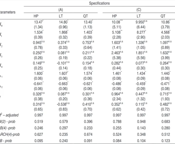
Table 5 – Estimates of Nonlinear Reaction Functions (17) and (19): 2004:1-2007:10
Parameters
Speciications
(A) (C)
HP LT QT HP LT QT
0
d 13.47*
(1.34) 14.80* (0.96) 13.40* (1.13) 10.08*** (5.11) 9.950n.s (6.44) 10.86* (3.79) 1
d 1.534
* (0.39) 1.868* (0.32) 1.403* (0.39) 5.108** (2.28) 8.277* (2.90) 4.568* (2.03) 2
d 0.945
n.s (0.78) 0.374n.s (0.33) 0.753n.s (0.64) 1.603n.s (1.41) 1.336n.s (1.05) 1.097n.s (0.89) 3
d 0.250
n.s (0.26) 0.081n.s (0.19) 0.211n.s (0.22) 2.463n.s (5.38) 1.851n.s (5.56) 1.632n.s (3.99) 4
d 0.149
n.s (0.25) -0.101n.s (0.14) 0.154n.s (0.18) 0.282n.s (0.44) 0.077n.s (0.30) 0.264n.s (0.30)
ρ 1
1.600* (0.06) 1.607* (0.06) 1.574* (0.06) 1.461* (0.08) 1.434* (0.09) 1.440* (0.08)
ρ 2
-0.641* (0.06) -0.663* (0.06) -0.621* (0.06) -0.486* (0.08) -0.459* (0.09) -0.471* (0.08)
α 0.326n.s
(0.38) 0.087n.s (0.20) 0.301n.s (0.36) 0.964n.s (2.34) 0.447n.s (1.32) 0.715n.s (1.93)
γ 0.316n.s
(0.65) -0.538n.s (0.83) 0.410n.s (0.70) 0.352n.s (0.62) 0.115n.s (0.42) 0.482n.s (0.72) R2 – adjusted 0.997 0.997 0.997 0.997 0.997 0.997 W(2) - prob 0.519 0.579 0.396 0.788 0.948 0.683 LB(4) -prob 0.246 0.297 0.233 0.255 0.143 0.280 ARCH(4)-prob 0.627 0.235 0.674 0.524 0.348 0.512
JB - prob 0.095 0.240 0.091 0.084 0.104 0.123
Notes: * Significant at 1%. ** Significant at 5%. *** Significant at 10%. n.s Nonsignificant. LB(4) refers
to the Ljung-Box statistic for serial autocorrelation of up to the fourth order. ARCH(4) re-fers to the LM-ARCH statistic for autoregressive conditional heteroskedasticity of up to the fourth order. jB refers to the jarque-Bera statistic.
Table 5 shows the estimates for the parameters of reaction functions (17) and (19), and for the coefficients of asymmetric preferences of the Central Bank.16,
17 In general, we observe that only the target estimated for the Selic rate, d 0, the
coefficient of response to the deviation of inflation from the target, d1, and the autoregressive coefficients, ρ1 and ρ2, were statistically significant. In addition, we did not find evidence that the Brazilian monetary authority has asymmetric prefe-rence over output above or below the target. Finally, we noted that the coefficient
16 Initially, we tried to estimate specifications (11), (14) and (16) using GMM in the reduced sample. However, we often had convergence problems or estimates for parameters that run counter to those predicted theoretically. Possible reasons for this may be the small sample size, the misspecification of the nonlinear model or the presence of weak instruments. Given these shortcomings, we decided to estimate only the reaction functions that include the deviation of inflation from the target at t-1 and of the output gap at t-2.
that measures the asymmetric preference over the stabilization of inflation, α, had a positive but not significant sign. This finding suggests that Central Bank’s asym-metric preferences over an above-target inflation may be associated with monetary policy actions taken in periods in which domestic crises strongly affected inflation and inflation expectations.
5 Conclusion
In this paper, we assessed possible asymmetries in the Central Bank’s objectives by estimating nonlinear reaction functions for the interest rate. To achieve that, we derived an optimal monetary policy rule taking into account an asymmetric loss function regarding positive and negative deviations of the output gap and of the inflation rate from the inflation target. Since the presence of asymmetries produces nonlinear responses of the interest rate to the deviations of the expected inflation from its target and from the output gap, we checked whether preferences are sym-metric by testing the null hypothesis of linearity of the reaction function. Also, we found the policymaker’s coefficients of asymmetric preferences by estimating the reaction function in its reduced form and verified whether they are significantly different from zero.
The empirical results showed that the Central Bank’s monetary policy decisions for the 2000-2007 period may be characterized by a nonlinear reaction function rela-tive to inflation, but linear relarela-tive to the output gap. Quite specifically, we found evidence that the Brazilian monetary authority has been more averse to negative rather than positive deviations of inflation from its target. As this behavior may result from policy decisions in periods of strong crises (as in 2001 and 2002), we estimated the coefficients of asymmetric preferences for the 2004-2007 period. The results for this reduced sample did not indicate the existence of any type of asymmetric preference regarding the stabilization of inflation and of the output gap.
References
BEC, F. et al. Asymmetries in monetary policy reaction function: evidence for the
U.S., French and German Central Banks. Studies in Nonlinear Dynamics and
Econometrics, v. 6, n. 2, 2002.
BLANCHARD, O. Fiscal dominance and inflation targeting: lessons from Brazil.
BLINDER, A. Central Banking in theory and practice. Massachusetts: The MIT Press, 1998.
BUENO, R. de L. da S. The Taylor rule under inquiry: Hidden states. In:
ENCON-TRO BRASILEIRO DE ECONOMETRIA, 27. Anais... Natal, 2005.
CALVO, G. Staggered prices in a utility-maximizing framework. Journal of Monetary
Economics, v. 12, n. 3, 1983.
CLARIDA, R. et al.Monetary policy rules in practice: some international evidence.
Cambridge: National Bureau of Economic Research, 1997. (Working Paper, 6254).
______. The science of monetary policy: a new Keynesian perspective. Cambridge:
National Bureau of Economic Research, 1999. (Working Paper, 7147).
______. Monetary policy rules and macroeconomic stability: evidence and some
theory. Quarterly Journal of Economics, v. 115, n. 1, 2000.
CUKIERMAN, A. The inflation bias result revisited. Tel-Aviv University, 2000.
Mimeo.
CUKIERMAN, A.; GERLACH, S. The inflation bias revisited: theory and some
international evidence. The Manchester School, v. 71, n. 5, 2003.
CUKIERMAN, A.; MUSCATELLI, A. Do Central Banks have precautionary
de-mands for expansions and for price stability? Theory and evidence. Tel-Aviv University, 2003. Mimeo.
______. Nonlinear Taylor rules and asymmetric preferences in Central Banking:
evidence from the United Kingdom and the United States. The B.E. Journal
of Macroeconomics, v. 8, n. 1, 2008.
DOLADO, j. j et al. Nonlinear monetary policy rules: some new evidence for the
US. Nonlinear Dynamics and Econometrics, v. 8, n. 3, 2004.
______. Are monetary-policy reaction functions asymmetric? The role of nonlinearity
in the Phillips curve. European Economic Review, v. 49, n. 2, 2005.
GERLACH, S. Asymmetric policy reactions and inflation. Bank for International
Settlements. 2000. Mimeo.
HANSEN, L. P. Large sample properties of generalized method of moments
estima-tors. Econometrica, v. 50, n. 4, 1982.
HOLLAND, M. Monetary and exchange rate policy in Brazil after inflation targeting.
In: ENCONTRO NACIONAL DE ECONOMIA, 33.Anais... Natal, 2005.
LIMA, E. C. R. et al.Monetary policy regimes in Brazil. Rio de janeiro: Instituto de
Pesquisa Econômica Aplicada, 2007. (Texto para Discussão, 1285a).
LUUKKONEN, R. P. et al. Testing linearity against smooth transition autoregressive
MINELLA, A. et al.Inflation targeting in Brazil: constructing credibility under ex-change rate volatility.Brasília: Banco Central do Brasil, 2003. (Trabalhos para Discussão, 77).
NETO, P. C. F. de B.; PORTUGAL, M. S. Determinants of Monetary Policy
Commit-tee Decisions: Fraga vs. Meirelles.Porto Alegre: PPGE/UFRGS, 2007. (Texto para Discussão, 11).
NEWEY, W. K.; WEST, K. D. A simple, positive semi-definite, heteroskedasticity and
autocorrelation consistent covariance matrix. Econometrica, v. 55, n. 3, 1987.
NOBAY, A. R.; PEEL, D. A. Optimal monetary policy in a model of asymmetric
Central Bank preferences. London School of Economics, 1998. Mimeo.
______. Optimal monetary policy with a nonlinear Phillips curve. Economics Letters,
v. 67, n. 2, 2000.
ORPHANIDES, A.; WIELAND, V. Inflation zone targeting. European Economic
Review, v. 44, n. 7, 1999.
POLICANO, R. M.; BUENO, R. D. L .S. A sensibilidade da política monetária no Brasil: 1999-2005. In: ENCONTRO NACIONAL DE ECONOMIA, 34.
Anais… Salvador, 2006.
RUDEBUSCH, G.D.Term structure evidence on interest rate smoothing and
mo-netary policy inertia. Journal of Monetary Economics, v. 49, n. 6, 2002.
SACK, B. Does the Fed act gradually? A VAR analysis.Washington, DC: Board of
Governors of the Federal Reserve System, 1998. (Finance and Economics Discussion Series, 17).
SACK, B.; WIELAND, V. Interest-rate smoothing and optimal monetary policy: a
review of recent empirical evidence. Journal of Economics and Business, v. 52,
n. 1-2, 2000.
SALGADO, M. j. S. et al. Monetary policy during Brazil’s Real Plan: estimating
the central bank’s reaction function, Revista Brasileira de Economia, v. 59, n.
1, 2005.
SILVA, M. E. A. da; PORTUGAL, M. S. Inflation targeting in Brazil: an empirical
evaluation. Porto Alegre: PPGE/UFRGS, 2001 (Texto para Discussão, 10). SOARES, j. j. S.; BARBOSA, F. de H. Regra de Taylor no Brasil: 1999-2005. In:
ENCONTRO NACIONAL DE ECONOMIA, 34.Anais... Salvador, 2006.
SROUR, G. Why do Central Banks smooth interest rates? Ottawa: Bank of Canada,
2001. (Working Paper, 17).
SURICO, P. The Fed's monetary policy rule and U.S. inflation: The case of asymmetric
preferences. Journal of Economic Dynamics and Control, v. 31, n. 1, 2007.
TAYLOR, j. B. Discretion versus policy rules in practice. Carnegie-Rochester
TELES, V. K.; BRUNDO, M. Medidas de política monetária e a função de reação do Banco Central do Brasil. In: ENCONTRO NACIONAL DE ECONOMIA, 34.Anais… Salvador, 2006.
VAN DIjK, D. et al. Smooth transition autoregressive models: a survey of recent
development. Econometric Reviews, v. 21, n. 1, 2002.
VARIAN, H. A Bayesian approach to real estate assessment. In: FEINBERG, S.E.;
ZELLNER, A.Studies in bayesian economics in honour of L. J. Savage.
Ams-terdam: North Holland, 1974.
______. Optimal interest-rate smoothing. The Review of Economics Studies, v. 70,
n. 4, 2003.
WOODFORD, M. Optimal monetary policy inertia. Cambridge: National Bureau
of Economic Research, 1999. (Working Paper, 7261).
_______________. Optimal interest-rate smoothing. The Review of Economics
Stu-dies, v. 70, n. 4, 2003.
Appendix A
Table A1 – Inlation Target: 1999-2008
Year Oficial target Tolerance interval Adjusted target
1999 8.0% ±2.0%
-2000 6.0% ±2.0%
-2001 4.0% ±2.0%
-2002 3.5% ±2.0%
-2003 4.0% ±2.5% 8.5%
2004 5.5% ±2.5% 5.5%
2005 4.5% ±2.5% 5.1%
2006 4.5% ±2.0%
-2007 4.5% ±2.0%
-Figure A1 – Selic Rate
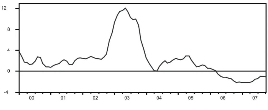
Figure A3 – Deviation of Inlation from the (Constant) Target