Estimating strategic complementarity in a state-dependent pricing model

Estimating Strategic Complementarity in a

State-Dependent Pricing Model

Marco Bonomo

EPGE, Getulio Vargas Foundation

Arnildo da Silva Correa

Central Bank of Brazil

Marcelo C. Medeiros

Ponti…cal Catholic University of Rio de Janeiro–Puc-Rio

EPGE/VALE 3rd Global Conference: Business Cycle

May 10, 2013

Macro Motivation

Monetary policy e¤ects depend on – the extent of price rigidity

– the type of friction:

adjustment cost ! state dependency ! little e¤ect information cost ! time dependency ! stronger e¤ect

– price complementarity: how a desired price depends on other prices

strong strategic complementarity in price ! stronger monetary policy e¤ect

Motivation: micro-macro conundrum

Micro evidence seems consistent with

– relatively high frequency of adjustments (Bils and Klenow 2004)

– state-dependency (Nakamura and Steinson 2008, Klenow and Kritsov 2008, Gagnon 2009)

Degree of strategic complementarity seems crucial to make it compatible with evidence that shocks (in particular monetary shocks) have important macro e¤ects: Gertler and Leahy (2008).

Indirect evidence from micro data based on model simulation:

– investigate whether speci…c channels are consistent with micro data:

– low degree or no strategic complementarity:

Klenow and Willis (2006) - real rigidities through demand side a la Kim-ball (1995), large relative price variation in BLS,

Burstein and Hellwig (2007) - prices and market shares from scanner data of a large grocery chain,

Krivtsov and Midrigan (2010) - inventory dynamics inconsistent with marginal cost rigidity.

This paper: what we do

Revisit the issue: what degree of strategic complementarity is consistent with micro data?

Direct estimation of strategic complementarity parameter in the frictionless price equation from ocurrence of price adjustments:

– Individual price adjustment data from Brazilian CPI of Getulio Vargas Foun-dation

p_i;t = + p_t + x0_t + ~_t + ~a_i;t S s c r* = p_i,t - p* Price decrease Price increase Time i,t i,t

This paper 2:- what we do

Price changes re‡ect frictionless optimal price variation but also the frequency of price adjustments. We disentangle those two e¤ects by assuming …rms follow a two-sided Ss rule (modeling selection):

– adjustments are triggered whenever the price discrepancy attains a certain threshold.

– it allows us to relate the price discrepancy (and conditional probability of adjusment) to the change in the frictionless optimal price since the last adjustment date.

– assumptions for non-observable idiosyncractic and aggregate shocks ! a relation between probability of adjustments and the conditional mean of changes in the frictionless optimal price since the last adjustment

With base on these assumptions and methodology we also: – recover the individual frictionless optimal price

This paper: how we do

Not based on closed model simulation

– The relations of the supply side of the economy are estimated without closing the model (Euler equation, monetary policy):

results should be robust to di¤erent speci…cations of the missing part.

We are agnostic with respect to the speci…c mechanism generating strategic complementarity

Main results 1

The parameter ranges from 0:03 to 0:10, implying a high degree of strategic complementarity.

This should lead to signi…cant real e¤ects of monetary shock:

– As suggested by Gertler and Leahy’s state-dependent model results with = 0:08.

Related literature

Related to Bils, Klenon and Mahlin (2009, 2011) who aim at isolating price rigidity from strategic complementarity with the following measures:

– theoretical reset price: the price the price-setter would choose if she could adjust.

– empirical reset price (di¤erent because of selection): assumes that reset price in‡ation for non-adjusters is equal to the one for adjusters.

– Compare empirical reset price measure of complete simulated models to the data.

Under Ss rules, frictionless price in‡ation=theoretical reset price in‡ation

Empirical reset price in‡ation re‡ects movements in the frictionless optimal price blurred by the selection e¤ect.

Results 2

We recover the frictionless optimal price:

– Frictionless price in‡ation less persistent than in‡ation and more persistent than reset price in‡ation and slightly less persistent than in‡ation ( = 0:51 > = 0:21 >. _b = 0:35).

– Frictionless price in‡ation has variability similar to in‡ation and much lower than reset price in‡ation. ( _b = 2:30% > _{= 0:76% '} = 0:72%)

– IRF of frictionless optimal price similar to BKM’s (2009) theoretical reset price in‡ation for state-dependent model with strategic complementarity.

Outline

Model

Empirical model and estimation

Data

Results

– Strategic complementarity – Pricing rules

– Actual, frictionless and reset in‡ation

Model

Illustrative model to derive frictionless optimal price equation. Several alterna-tive speci…cations lead to the same equation.

Households: the representative household seeks to maximize

E0 8 < : 1 X t=0 t 2 4U_tC 1 1 t 1 1 Z ₁ 0 V_i;tL1+_i;t 1 + di 3 5 9 = ;; where C_t = "Z ₁ 0 C ( 1)= i;t di # _{= 1} : (1)

– Demand for individual product:

C_i;t = C_t Pi;t P_t

!

– Labor supply: V_i;tL_i;t U_tC 1 t = Wi;t P_t (3)

Firms: Continuum of monopolistically competitive …rms supplying di¤erenti-ated goods.

– Production function for …rm i:

Y_i;t = A_i;tL_i;tM_t(1 ); (4)

M_t - foreign input

– Exogenous real exchange rate - E_t:

Model 2

– Assume for simplicitly that exports and imports are equal. Equilibrium: Y_t = C_t

– Real marginal cost function:

(Y_i;t; Y_t; E_t; V_i;t; U_t; A_i;t) =

A 1+ 1+ (1 ) i;t Y 1+ (1 ) it Y 1 (1+ (1 )) t E (1 )+ (1 ) 1+ (1 ) t V 1+ (1 ) i;t U 1+ (1 ) t (5) where " (1 )# 2 (1 ) 1+ (1 )

Model 3: Frictionless optimal price

Frictionless optimal price: Firms maximize pro…ts subject to demand and cost yielding:

P_i;t

P_t = (Yi;t; Yt; Et; Vi;t; Ut; Ai;t); (6) where =( 1)

– Substituting the marginal cost expression (5) into the markup rule (6) and taking the log of the resulting expression yields:

where + 1 1 + [(1 ) + ] (1 + ) (1 ) 1 + (1 ) + ~ a_i;t 1 + 1 + (1 ) + ai;t + 1 + (1 ) + vi;t ~ t 1 + (1 ) + ut 1 + (1 ) 1 + (1 ) + log :

Model 3: Frictionless optimal price

When < 1, strategic complementarities in price setting.

The degree of strategic complementarity depends:

– positively on (elasticity of intertemporal substitution)

– negatively on (elasticity of product with respect to labor), and (elasticity of substitution among alternative varieties).

– assuming 1 1, as usual in the literature, positively on (the inverse of the Frish elasticity of labor supply)

Di¤erent mapping depending on details of structural model: homogenous labor markets leads to

= +

1

Model 4: Price rigidity model

We want to estimate 7, but observe infrequent price changes.

To bridge the gap: a state-dependent model of price rigidity.

We assume …rms follow Ss pricing rules parametrized by (s; c; S) - just pos-tulated, but can be rationalized

– state variable: price discrepancy

r_i;t p_i;t p_i;t: – adjustment rule: 8 > < > : c s if r_it s 0 if s r_it S (S c) if r_it S (8)

Empirical model

r_i;t p_i;t p_i;t (9)

= p_{i; i;t} p_i;t = c + p_i;

i;t pi;t;

Rewrite p_it as:

p_i;t = + x0_t + ~_t + ~a_i;t

Substituting our model for p_it: r_i;t = c + + x0

i;t + ~ i;t + ~ai; i;t + x0t + ~t + ~ai;t

= c + x _i;t x_t 0 + ~

i;t ~t + ~ai; i;t ~ai;t

= c z0_i;t ~_t ~

i;t a~i;t a~i; i;t (10)

Empirical model 2: speci…cation of shocks

Aggregate shock: ~ t = ~t 1 + vt; vt IID(0; 2_v): (11) Idiosyncratic shock: ~ a_i;t = a_i + a_i;t

Empirical model 3

Under these assumptions:

r_i;t = c _i;t z0_i;t

t X j=t _i;t+1 v_j u_i;t = c _i;t z0_i;t T X j=1 jdi;t (j) ui;t; where i;t t i;t ; d_i;t (j) = 8 < : 1; _{if j 2} ht _i;t + 1; ti 0; otherwise : (13) and u_i;t t X j=t _i;t+1 "_{i;j N}(0; _i;t 2):

Empirical model 4

De…ne the observable variable r_i;t as

r_i;t = 8 > < > : 1; if p_i;t > p_{i;t 1} 0; if p_i;t = p_{i;t 1} 1; if p_i;t < p_{i;t 1} : (14)

De…ne w_i;t = ( _i;t;z0_i;t;d_i;t0 )0, where d_i;t = (d_i;t(1) ; :::; d_i;t (T ))0

Then:

Empirical model 5

P r[r_{i;t = 1j}w_i;t] = P r[r_{i;t sj}w_i;t] = P r[c _i;t z0_i;t

T

X

j=1

jdi;t (j) ui;t sjwi;t] (15)

= P r

2 6

4qui;t

i;t

c s _i;t z0_i;t PT_{j=1 j}d_i;t (j)

q i;t 3 7 5 = 1 0 B @c sq1 i;t q i;t z0_i;t q i;t T X j=1 jdi;t(j) q i;t 1 C A = 1 0 @ ₁•_{1i;t ~•i;t z•}0 i;t~ T X j=1 ~_jd•_i;t (j) 1 A

variables with two dots are divided by q _i;t;

Empirical model 6: ordered probit model

Probability of price increase:

P r[r_{i;t = 1j}w_i;t] = 1 0 @ ₁•_{1i;t ~•i;t z•}0 i;t~ T X j=1 ~_jd•_i;t (j) 1 A

Probability of keeping the price:

P r[r_{i;t = 0j}w_i;t] = 0 @ ₁•_{1i;t ~•i;t z•}0 i;t~ T X j=1 ~_jd•_j;t 1 A ... 0 @ ₀•_{1i;t ~•i;t z•}0 i;t~ T X j=1 ~_jd•_i;t(j) 1 A

Probability of price decrease:

P r[r_i;t = _1jw_i;t] = 0 @ ₀•_{1i;t ~•i;t z•}0 i;t~ T X j=1 ~_jd•_i;t (j) 1 A

Empirical model 7: estimation

Estimation by quasi-maximum likelihood controling for:

– dependence on the cross-section due to common macro shocks

– autocorrelation and heteroskedasticity that emerge from structural model

Robust variance-covariance matrix with non-parametric correction à la Newey-West.

Asymptotics: – N ! 1

Empirical model 8: identi…cation

Real rigidity parameter:

= ~1 ~ 1 + ~2 : (16) = 1 ~ 1 + ~2 : (17)

Pricing rule parameters:

c S = ₁

S c = ₀ S s = ( _{1 0})

Data: microdata

Price quotes from Brazilian CPI calculated by FGV, from 1996 to 2006.

Typical item: type 1 rice of the Combrasil brand, sold in a 1kg package in a given outlet, in Rio de Janeiro.

Each item is surveyed once a month in Rio and São Paulo.

Characterization of price-setting using Brazilian micro data: – Gouvea (2007) uses this same sample;

– Barros, Bonomo, Carvalho and Matos (2010) uses the whole FGV CPI from 1996 to 2010.

Treatment:

– sales V …lter

– exclude products with problematic price quotes (Eichenbaum et al 2012)

After exclusions we were left with 178 products and services with all seven sectors still represented, accounting for 40.4% of all prices in the CPI-FGV.

Results 1: Baseline estimation

Yt pt et Conf. int for

0:60

Results 2: Robustness

Model _Yt p_t e_t C. i. for Period 1997 - 2000 0:15 (0:160) (0:146)4:93 (0:024)0:62 (0:031)0:03 0:03 0:09 Period 2001 - 2004 1:29 (0:094) (0:054)11:07 _(0:015)0:40 (0:007)0:10 0:09 0:12

Without Exchange Rate 2:93

(0:074) (0:037)3:43 (0:008)0:46 0:44 0:48

Idiosyncratic White Noise 0:90

(0:112) (0:072)12:72 (0:018)0:05 (0:008)0:07 0:05 0:09

Without promotions 0:53

(0:079) (0:050)8:90 (0:013)0:02 (0:008)0:06 0:04 0:07

Without exclusions 0:44

Results 3: pricing rule

0 = c S 1 = c s c s S c Size of in. range

0:92

(0:01)

0:62

(0:01) (0:01)0:10 0:06 0:09 0:15

reasonable (same value obtained by Klenow and Willis without strategic complementarity).

negative adjusments are larger than positive adjustments, as in the sample.

adjustments sizes are smaller than in the sample:

– estimation does not use adjustment size, but frequency of adjustments – downward bias due to heterogeneity and nonlinearity in the relation size

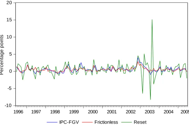
Results 4: actual, frictionless, and reset price in‡ation

We compare statistics of: – actual FGV CPI in‡ation

– frictionless in‡ation - in‡ation that would occur if there were no nominal rigidities:

recovered with base on our estimation of p equation;

in our setup (Ss rules) coincides with theoretical reset price in‡ation. – empirical reset price in‡ation ^ , proposed by Bils, Klenow and Mahlin

(2009), which is di¤erent from the theoretical reset price in‡ation due to selection of price changers.

Empirical reset price

^

p_i;t =

(

p_i;t; if p_{i;t 6= pi;t 1} ^

p_{i;t 1} + ^_t; if p_i;t = p_{i;t 1} ; (18) where ^_t is given by:

b_t

P

i

!_i;t p_i;t p^_{i;t 1} I_i;t

P

i

-10 -5 0 5 10 15 20 1996 1997 1998 1999 2000 2001 2002 2003 2004 2005

IPC-FGV Frictionless Reset

P e rc e n ta g e p o in ts

Note: Frictionless inflation corresponds to the average obtained across the 1000 simulations. Actual inflation is calculated among products left after exclusions. Reset inflation is obtained using BKM's methodology.

Actual, frictionless and reset price in‡ation

Series Std deviation Persistence

Actual In‡ation IPC-FGV 0:76% 0:51 Frictionless In‡ation 0:72% 0:21

Results 5: IRFs of frictionless, and reset price in‡ation

Following BKM we estimate an AR(6) for and ^ and graph a IRF for p and pb following a 1% impulse:

– IRF for p is upward sloping, which is consistent with strong strategic com-plementarities.

Results 5: IRFs of actual, frictionless, and reset price

in-‡ation

0 1 2 3 4 5 6 1 2 3 4 5 6 7 8 9 10 11 12 P e rc e n ta g e p o in ts

Note: Accumulated response of actual inflation to one unit innovation. Months

Results 5: IRFs of frictionless, and reset price in‡ation

0.0 0.2 0.4 0.6 0.8 1.0 1 2 3 4 5 6 7 8 9 10 11 12

Note: Accumulated response of reset price inflation to one unit innovation. Months P e rc e n ta g e p o in ts

Evaluating results

Properties of ^ are similar in US and Brazilian data

is less variable and more persistent than ^ :

– ^ is in‡uenced by the selection e¤ect, but not (where Ss rules took care of it)

– re‡ects more directly strategic complementarity

Conclusions

Direct estimation of complementarity parameter with base on micro data: – need to assume some pricing rule

– does not depend on the demand side

Strong strategic complementarities found in micro data.

– we did not use macro e¤ects of shocks in the estimation; – could lead to signi…cant macro e¤ects.

Our methodology recovers frictionless optimal price: – a fundamental variable.