BASSILO

(1)

Faculdade de Engenharia da Universidade do Porto

Battery storage sizing and location in distribution

systems

Tiago João Amorim Abreu

Mestrado Integrado em Engenharia Eletrotécnica e de Computadores

Major Energia

Supervisor: Vladimiro Miranda (Full Professor)

(2)

(3)

iii

The very essence of instinct is that it's followed independently of reason. Charles Darwin

(4)

(5)

v

Resumo

Esta tese aborda o problema de dimensionamento, localização e operação de armazenamento de energia não doméstico disperso em redes de distribuição, mais especificamente, baterias elétricas. Estas, são integradas na rede juntamente com geração fotovoltaica distribuída, com o objetivo de analisar seu potencial exploratório no negócio de energia. Para o efeito, foi proposta uma formulação híbrida utilizando programação linear, na otimização da operação das baterias e a meta-heurística EPSO, Evolutionary Particle Swarm Operation, para a minimização dos custos do dimensionamento, localização e escolha da interface tecnológica de baterias em vários pontos de uma rede elétrica de distribuição.

Um modelo estocástico para a simulação das cargas, preço de energia e geração fotovoltaica foi também desenvolvido para simular o que funcionamento da rede de distribuição ao longo da vida útil dos sistemas de armazenamento.

Os resultados apresentados são para uma rede de energia real, CIGRE - rede de distribuição de MT europeia, modificada para ser operada como rede radial, compreendendo cargas distribuídas (comercial e residencial) e geração fotovoltaica, em que a variação do preço da energia, é considerada para validar o modelo de exploração de negócios proposto.

(6)

(7)

vii

Abstract

This thesis addresses the problem of sizing, locating and operating non-domestic energy storage in distribution networks, more specifically, electric batteries. These are included into a network with distributed photovoltaic generation, with the objective of analyzing their exploratory potential in the energy business. To accomplish this, a language based on linear programming and EPSO metaheuristics, a Swarm Operation of Evolutionary Particles, was proposed to minimize the costs of integrating batteries in several points of a distribution network.

Given the sizing and location of each battery, linear programming is used to determine the optimal operation of the energy storage system for a multi-day scenario. A stochastic scenario model was also created to simulate the load, generation and energy prices data over time. EPSO will then use the operation given by this optimization to evaluate the costs of inserting batteries in the network over their life span.

Results will be presented for a real distribution network, the CIGRE MV benchmark network, modified to be used in its radial configuration, using distributed loads (commercial and residential) and photovoltaic generation. Energy price variation is considered to evaluate the model proposed

(8)

(9)

ix

Acknowledgements

I would like to express my gratitude to Professor Vladimiro Miranda for the opportunity to work in such an interesting subject and for his valuable insights and guidance throughout the months on which this thesis was devised.

I would also want to thank INESC TEC for embracing me into their offices while I was doing this investigation and for providing me with the data that would allow to test and prove the model created.

As for my colleague and friend that accompanied me in this adventure, Piedy Agamez Arias, I would like to thank you for all the hours of work that we spent together in the research of the model presented.

A special note of gratitude must be given to my friends, which for the last 5 years shared their lives, motivated me and showed me the best of the best that the future of engineering has to offer.

To my parents and family, I want to acknowledge all their support and love that allowed me to face the good and the bad moments in all my academic and non-academic moments.

Finally, I would like to thank my beloved Ana Patrícia, for all the help, the proofing and correcting every single phrase in this thesis and for all the moments that were and will be shared, v.c.e.i.

(10)

(11)

xi

List of figures

Figure 2.1: Battery Scheme [1] ... 4

Figure 2.2: Battery technologies and other energy storage systems and their uses. [3] ... 5

Figure 2.3: EPSO scheme ... 8

Figure 3.1: Possible Seasons probabilities ... 11

Figure 3.2: Price curves for each season. ... 12

Figure 3.3: Probability of occurrence for each weather condition scenario for each season. . 12

Figure 3.4: Cumulative function and choosing area for each season. ... 13

Figure 3.5: Scheme of the Season selection process. ... 13

Figure 3.6: Scheme of the weather selection process. ... 14

Figure 3.7: Decision Scheme for the year scenario model. ... 14

Figure 4.1: Scheme for the uses of the optimization techniques. ... 15

Figure 4.2: Proposed particle structure. ... 16

Figure 4.3: Proposed algorithm to optimally locate batteries using EPSO ... 19

Figure 4.4: Battery operation scheme regarding SoC evolution over time. ... 20

Figure 5.1: Topology of MV Distribution network benchmark... 24

Figure 5.2: Seasons probabilities. ... 25

Figure 5.3: PV Generation Behaviour in Bus 4 for a year. ... 25

Figure 5.4: PV Generation Behaviour in Bus 4 for 10 days. ... 26

Figure 5.5: Load in Bus 4 over a year ... 26

Figure 5.6: Load in Bus 4 over 20 days. ... 27

(14)

Figure 5.8: Energy Prices over 10 days ... 27

Figure 5.9: Battery State of Charge (0.7 Charge/Discharge Rate) and Energy Price over 1 Day. ... 29

Figure 5.10: Battery State of Charge (0.7 Charge/Discharge Rate) and Energy Price over 10 Days. ... 29

Figure 5.11: Size and Charge/Discharge rate for 10 particles used in the model with 1MW maximum size ... 30

Figure 5.14: Size and Charge/Discharge rate for 20 particles used in the model ... 32

Figure 5.15: Size and Charge/Discharge rate for 50 particles used in the model ... 32

Figure 5.16: Costs function evolution of each case presented. ... 33

Figure 5.17: Optimization for the 10MW maximum size case. ... 34

Figure 5.18: Costs function evolution of the maximum 10MW size case ... 34

Figure 5.19: Solutions using 20 particles in the model's optimization. ... 35

Figure 5.20: Solutions using 10 particles in the model's optimization. ... 35

(15)

xv

List of tables

Table 2.1: Literature Review ... 10

Table 5.1 Power Electronics Costs ... 28

Table 5.2: Dispersal results for each case. ... 36

Table A.1 Network’s line parameters. ... 39

Table A.2 Network sensitivity matrix ... 39

Table A.3: Winter's Load Data ... 40

Table A.4: Spring/Autumn's Load Data... 41

Table A.5: Summer's Load Data ... 41

(16)

(17)

xvii

Abbreviations and Symbols

List of abbreviations

AC Alternating Current BESS Battery Storage System

DC Direct Current

EPSO Evolutionary Particle Swarm Optimization ESS Energy Storage System

HVN High Voltage Network

MV Medium Voltage

OPF Optimal power flow

PSO Particle Swarm Optimization PV Photovoltaic generation SoC State of Charge

List of Symbols

β random weather scenario value 𝑏 best global value

𝑏 best value of a given particle 𝐵𝑔 , battery as generator value in k an p

𝐵𝑙 , battery as load value in k an p

𝐶 system communication value 𝑐 battery charge over 𝑝

CA cloudy in the afternoon probability CD cloudy day probability

CM cloudy in the morning sky probability CS clear sky probability

𝑑 battery discharge over 𝑝

(18)

𝐼 current in a line

𝑘 bus

𝑛 location

𝑁(0,1) normal distribution

𝑝 period

𝑃 , power flow in period p

𝑝 power loss in a line 𝑅 Resistance in line ik 𝑠𝑖𝑧𝑒𝑛

battery size

S Number of solutions

s solution

𝑉 velocity in a given iteration 𝑋 particle in a given iteration

𝑤 weight parameter

𝜏 induced parameter tau

(19)

Chapter 1 Introduction

As environmental and geopolitical concerns against the usage of hydrocarbons to produce electric energy increase, the propagation of renewable energy generation such as photovoltaic arrays were inserted into the distribution network. Although this minimizes the needs of hydrocarbon-based energy generation, the intermittent nature of renewable energy introduces concerns in stability, power quality and reliability of the system.

The use of energy storage systems can reduce these issues in distribution networks and can diminish the link between energy demand and energy generation that comes from far away power stations. Power quality and the stability of the power output can also be improved with the use of energy storage systems. Power electronic technologies take also an important role in the optimization of these storage systems. With different power electronic available to the energy network operator, there are several configurations of energy storage systems that can be applied.

Optimization tools such as Gurobi are used to find the solution of the best use of these technologies. However, as they are not created with the single purpose to optimize this specific objective, they require heavier computation processing than an optimization tool that is moulded to this problem.

The objective of this thesis is to analyse the viability of the business model of introducing batteries dispersed in distribution networks, in the optic of the network operator. To accomplish this, it is proposed a hybrid combining the meta-heuristic evolutionary particle swarm optimization for sizing, location and interface technology selection and linear programming for optimizing battery’s operation. This research work includes the development of a MATLAB tool that implemented the proposed model and validated using a real distribution network.

(20)

(21)

Chapter 2 State of Art

2.1. Energy Storage Technologies

2.1.1. Energy Storage Systems Used in Power Networks

Energy can be stored in energy storage systems, ESS, when power production is greater than consumption. However, as the energy network operates in alternating current, AC, ESS cannot save electrical energy directly. This means that it needs to be stored in other forms, such as electrochemically, magnetically, as potential energy or as compressed air. The batteries that are used in this thesis are a type of electrochemically storage and as so, this technology is going to be exposed in this subchapter.

2.1.2. Electrochemical Storage Systems

From all of the technologies mentioned in subchapter 2.1.1, electrochemical storage is the most cost-efficient available [1]. There are two main kinds, capacitors and batteries. These technologies use two electrodes, an electropositive electrode, the anode, and an electronegative electrode, the cathode. From the anode, electrons flow on charge through a circuit into the cathode. To balance this flow, it is used an electrolyte, liquid or solid, which only allows for the flow of ions and not electrons. The figure below illustrates this process.

(22)

4 State of Art

The difference between capacitors and batteries lies in the processes used to store energy. In the first one, energy is stored as surface charge whereas in the second one, electrical energy is stored as chemical energy.

In capacitors, it is required a large amount of surface area, as the storage capacity is directly linked to the surface area. In batteries, chemical reactions will occur all through the bulk of the solid, which means that the material used must be devised to permit the admittance of reacting species throughout the material and to conceive its removal. This process needs to occur thousands of times so that there is a commercially viable battery.

There is also a hybrid technology that uses the best of the two technologies, called supercapacitors. The supercapacitors use surface charge as well as some faradaic reactions in the bulk of the material [2].

2.1.3. Battery Storage Systems (BESS)

Currently, from the electrochemical technologies mentioned, BESS are the technology used in the power network to store energy. However, there are also several types of battery technologies. These technologies are used in power quality, in the transmission and distribution and in bulk power systems.

Each one of these technologies presents different qualities that can be applied to different situations (figure 2.2).

(23)

5

1. Lead-Acid Batteries:

The lead-acid batteries possesses a low specific energy due to its weight [3], it is adopted into situations where costs are an important factor and its low energy density is not. Its application goes from 1kW to 10MW [4].

2. NiCd/NiMH Batteries:

The NiCd battery uses a cadmium negative electrode as well as a nickel oxide-hydroxide positive electrode, a separator and an electrolyte. This technology has a lower energy density, having its application from 1kW to 0.5MW [4]. It has environmental hazards, so they have been replaced for NiMH batteries. They possess better energy density, being able to be used from 1kW to 1MW [4]. The downside of NiMH batteries is that they have a high self-discharge rate, the possibility of a cell rupture due to very high charge rate and also the possibility of reverse polarization of the cell due to being discharged [4], [5].

3. Li-Ion Batteries

This type of batteries possesses a high energy density and a low discharge rate. They are made from positive Li-ions that migrate from the negative plate to the positive plate during

(24)

6 State of Art

the discharge and the reverse path is taken when charging. The negative plate is made of graphite and the positive plate is made from an alloy containing lithium. Their main disadvantage is that the internal resistance can heat, causing battery failure [6].

4. NaS Batteries:

NaS batteries operate normally in temperatures that ranges from 300ºC to 350ºC. It is used a sodium negative electrode that oxides at the surface during the discharge and forming sodium ions. They will then migrate through a solid electrolyte made of a beta-alumina that is reduced and generates sodium pentasulfide, Na2S5. The electrolyte conducts almost no electrons, having

a low rate self-discharge. These batteries contain hazardous elements that can ignite in contact with water. Their range of application varies between 0.8 MW and 10 MW [4].

5. Flow Batteries

There are several types of flow batteries such as Iron-chromium, zinc-bromine and zinc-air batteries. Their general operation principle uses its electrolyte outside the cell in two separate tanks and depletes the two different electrolytes that are pumped into the cell. They are separated through a proton exchange membrane that permits the circulation of ions. These type of batteries have application from 10kW to 10 MW [4].

2.2. Meta Heuristic Methods

Meta heuristic methods are commonly known as algorithm-based optimizations that presume its problem-solving equations from biological processes found in nature. These are of great utility when used in the resolution of problems of combinatorial nature, with the possibility of application in a wide range of fields. In power systems, meta-heuristics have a considerable potential to solve planning and operation-based problems. The optimal sizing and location of batteries is an elaborate problem that encompass the nature of these meta heuristics. In the section below, it will be given a description of

Particle Swarm Optimization,

PSO, and of

Evolutionary Particle Swarm Optimization, EPSO.

2.2.1. Particle Swarm Optimization

PSO concept revolves around the laws of movement of a swarm or a bird flock. It implies that, at a given iteration, there must be a set of solutions called “particles” [7]. From one iteration to another, each particle advances accordingly to its “velocity”.

(25)

7

If we take 𝑋 as a particle in a given iteration, 𝑉 as the velocity of said particle, the movement rule will be defined as the following:

𝑿_𝒊𝑵𝒆𝒘_{= 𝑿}

𝒊+ 𝑽𝒊𝑵𝒆𝒘 (2.1)

where 𝑉 is formulated as:

𝑽_𝒊𝑵𝒆𝒘_{= 𝑫𝒆𝒄(𝒕)𝒘}

𝒊𝟎𝑽𝒊+ 𝑹𝒏𝒅𝟏𝒘𝒊𝟏(𝒃𝒊− 𝑿𝒊) + 𝑹𝒏𝒅𝟐𝒘𝟐(𝒃𝒈− 𝑿𝒊) (2.2)

Considering 𝑏 as the best point found by the particle in its past life and 𝑏 as the characterized best point found by the swarm.

𝑉 can be divided in three factors. Inertia or habit, first term of the summation, which represents that the particle keeps the motion of previous iterations. Memory, represented in the second term, enacting the attraction of the particle to the best point in its trajectory. Cooperation/information exchange between particles is the last term of the summation, that embodies the attraction to move unto the best point found by the swarm.

The parameters 𝑤 can be considered as fixed weights or as evolving with the iterations of the optimization by following a function introduced by the user, set at the beginning of the process. 𝑅𝑛𝑑 are random numbers sampled from a uniform distribution in [0,1]. Dec(t) is a function decreasing as the iterations develop, reducing progressively the importance of the inertia term.

2.2.2. Evolutionary Particle Swarm Optimization

EPSO blossomed from the idea of associating to the PSO scheme the selection procedure and genetic algorithm into its parameters [8]. In this formulation, the variables will fall into the Evolution Strategies community vocabular and are divided into the object parameters, X variables, and strategic parameters, w weights. For each iteration, it will be considered a set of alternatives to the solution that we will call particles. Every particle will be created with object and strategic parameters [X,w]. EPSO will then follow the same blueprint.

REPLICATION – each particle will be replicated r times; MUTATION- each particle has its weights w mutated;

REPRODUTION – each particle generates an offspring according to the particle movement rule (2.1.);

EVALUATION – each offspring has its fitness evaluated;

SELECTION – by stochastic tournament, the best particles of the swarm will endure to form a new generation.

(26)

8 State of Art

EPSO velocity equation resembles the one used in PSO (2.1), however, the weights now are not previously set, but mutated in every iteration in the mutation process [9]. The equations for the velocity and mutation are as follow:

𝑽_𝒊𝑵𝒆𝒘_{= 𝒘}

𝒊𝒐 ∗_𝑽

𝒊+ 𝒘𝒊𝟏∗(𝒃𝒊− 𝑿𝒊) + 𝑪 ∗ 𝒘𝒊𝟐∗(𝒃𝒈− 𝑿𝒊) (2.3)

𝑤∗ _{= 𝑤 + 𝜏𝑁(0,1)} _(2.4)

The global best can also be mutated using the same mutation equation used for the weights

𝑏∗_{= 𝑏 + 𝜏 𝑁(0,1)} _(2.5)

where 𝜏 and 𝜏 can be fixed weights or even treated as strategic parameters therefore can be mutated [8].

To replicate the effects of the lack of communication between members of the swarm, a factor C can be introduced in the equation 2.3, [10]. C will act as a binary variable equal to 1 with a given communication probability p or 0 with a probability (1-p). p is determined by the user of the model [11].

(27)

9

2.3. Batteries’ Sizing, Location and Operation Optimization

The proper size and location of batteries as its operation is a subject of great importance in the energy transmission and distribution networks. Several optimizations were proposed over the course of the years for battery’s sizing, location and operation, although, in most of the work found, only one or two of this problems is tackled. Nonetheless, in the following paragraphs, highlights from the main conclusions of the publications review are going to be summarized.

In [12] Borowy and Salameh proposed a methodology to minimize costs of sizing a battery bank by applying a probability database that allows the calculation of the best number of sizing of the battery bank, PV arrays for a PV/wind stand-alone system.

Using dynamic programming [13], an approach for the optimization of power flow by increasing the penetration of PV production into the network is suggested. This was carried out by doing simulations for real conditions over the course of one exemplary day.

In the paper published by Choi, Kim and Seo [14], an optimization for a hybrid storage system using batteries and supercapacitors is introduced with the objective of minimizing magnitude/fluctuation of the current that flows in and out of each battery and the minimizing energy loss in the supercapacitator system.

Po-Hung Chen [15] created a methodology that applied EPSO into the pumped-storage scheduling. It was also compared to other optimization methodologies such as PSO, Genetic Algorithm and Dynamic Programming, to which it was concluded that EPSO had the best results, with a better cost saving than the other techniques.

A new meta-heuristic based in PSO is presented by Lee [16]. The Multipass Iteration Particle Swarm Optimization Approach is used to determine the best schedule for a battery energy storage system, regarding wind turbine generators, for a time of use rate. The results are also compared to PSO Dynamic Programming and Genetic Algorithm.

A hybrid of Tabu Search and PSO was used in the paper written by Mahdi Sedghi, Ali Ahmadian and Masoud Aliakbar-Golkar to find optimal storage planning [17]. The wind power distributed generation and wind power uncertainty were considered in this work to search the optimal storage planning.

A table with the authors, type of problem, objective and method of accomplish the goals is available bellow to better emphasize the works mentioned above.

(28)

10 State of Art

Table 2.1: Literature Review

Authors Type of Problem Objective Method

Bogdan S. Borowy, Ziyad M. Salameh [12]

Sizing of Battery Bank and the PV array for a stand-alone system

To develop a methodology for calculating the optimal size of batter bank and PV

array for a stand-alone hybrid Wind PV system

Minimization of Cost function by using probability cases from a database Yann Riffonneau, Seddik Bacha, Franck Barruel, and Stephane Ploix [13]

Optimal Power Flow Management

Help intensive penetration of

PV production into the network Dynamic Programming Mid-Eum Choi, Seong-Woo Kim, and Seung-Woo Seo [14] Reduce the magnitude/fluctuation

of the current flowing in and out of the battery and the energy

loss seen by the SCs

Energy Management Optimization to reduce the

magnitude/fluctuation of the current flowing in and out of the battery and the energy loss seen by the SCs

Matlab Simulations using Solver Po-Hung Chen [15] Pumped-Storage

Scheduling Minimize costs EPSO

Tsung-Ying Lee [16]

Operating Schedule of Battery Energy Storage

System

Reach the minimum electricity charge Multipass Iteration Particle Swarm Optimization Mahdi Sedghi, Ali Ahmadian and Masoud Aliakbar-Golkar [17]

Storage Planning for

BESS Minimizing operation Costs

Hybrid Tabu Search and Particle Swarm Optimization Steven D. Percy, Mohammad Aldeen, Christopher N. Rowe, Adam Berry [18] Optimization Methodolgy

Analysis of the optimal capacities of residential

battery systems

Multi-Period Linear Program

(29)

11

Chapter 3 Stochastic Scenarios

For the operation of the proposed method of optimizing the sizing, location, operation and best power electronic technology of batteries it is required to introduce values of generation, load and energy price in the network. This was achieved by constructing a stochastic scenario model, so that the optimization can be tested. This makes it also possible to implement, in future works, prediction models to replace the stochastic scenarios as the variables will already be set up.

For the construction of the stochastic scenarios, data for typical prices and load was gathered from EDP Distribuição public records [19] and photovoltaic generation (PV) was provided by INESC TEC [20]. The data gathered was implemented in sets of three hours, having the daily curves been divided into 8-point curves.

3.1. Scenarios Generation

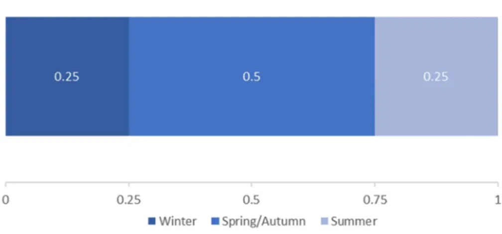
Data was divided into three seasons: Summer, Winter and Spring/Autumn, with an incidence of 25%, 25% and 50% respectively.

(30)

12 Stochastic Scenarios

In every season, the typical daily load and price curves were set by the analysis of the average daily curves for each respective months where price and load average behaviours are similar. Load data was inserted by adding residential and commercial curves into one singular curve to ease the implementation of these values in the program created. This curve is then used to create load values for the different buses of the power network. Price curves are set as an average of the daily price curve for the months in each season (Figure 3.2).

As for PV generation, its daily generation depends directly on the weather conditions. From the data gathered and through the analysis of the weather behaviour for every season, four weather scenarios were constructed and the occurrence probability was determined. In the following figure, the scenarios and their probability for each season are illustrated.

Figure 3.3: Probability of occurrence for each weather condition scenario for each season. Figure 3.2: Price curves for each season.

(31)

13

3.2. Day and Year Scenario Setting

3.2.1 Day Scenario

For the day scenario determination, it is generated a random value (α) with equal probability distribution between zero and one. This number is then inserted and compared to the cumulative probability function of the seasons in the following order: Winter, Spring/Autumn and Summer. This determines which season will be used for gathering information.

If α is a value less or equal to the winter’s probability, the season chosen is Winter. If α greater than winter’s probability and lesser or equal to the summation of winter and spring/autumn probability, spring/autumn season is selected. If the value is greater than this probability, summer is chosen (figure 3.5).

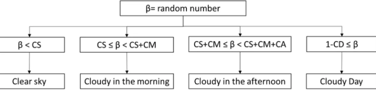
Load and Price information are then saved in the database used in the model. As for PV generation, a new random value (β) is required to select the weather condition scenario used for the season chosen. This new value with follow the same type of scheme used for the season

Figure 3.4: Cumulative function and choosing area for each season.

(32)

14 Stochastic Scenarios

selection. However, probability of each weather condition scenario depends on the season selected.

For each season, CS is the clear sky probability, CM is the cloudy in the morning probability, CA is the cloudy in the afternoon probability and CD is the cloudy day probability. The total of the previous variables is equal to one, as can be seen in the equation

𝑪𝑺 + 𝑪𝑴 + 𝑪𝑨 + 𝑪𝑫 = 𝟏 (3.1)

The scheme that follows explains how the scenario is selected by using these probabilities.

3.2.2 Year scenario

The decision process used in the day scenario can be replicated for 365 days. By doing this, a database for load, weather and prices is created, which simulates the use of a prediction model in the optimization model proposed.

Figure 3.6: Scheme of the weather selection process.

(33)

Chapter 4 EPSO and Linear Programming Methods

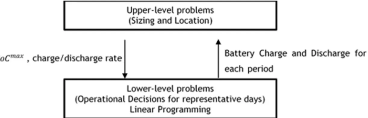
During the course of this work, a software tool to optimally size, locate batteries and choose interface technology was developed using a MATLAB environment that uses a mixture of meta heuristic and linear programming. These two methods of optimization are used to solve different problem levels in the program. In the upper level problem, EPSO is used in the sizing and location of batteries whereas linear programming is used in the lower level problem to find the best operation for each battery that is inserted in the network for each iteration of EPSO. There is data being interchanged between the upper and lower level of optimization. From EPSO the Lower level problem receives charge/discharge rate and size of each battery. From there on, the result of this optimization gives to EPSO the costs of operating each battery [21]. This process is illustrated in following figure.

In this chapter, it will be given the description of how each one of these methods was implemented and the assumptions made.

(34)

16 EPSO and Linear Programming

4.1. Sizing and Location Using EPSO

The optimal location of batteries is an intricate problem that can be solved using EPSO. The model proposed considers the possibility of introducing a various number of batteries in a set of previously determined sites, in a power network. In each location it can be placed a battery of a determined dimension and technology. In the proposed model, each particle of the swarm represents a possible solution to the location problem [22]. The length of each particle is defined by the double of the number of candidate locations, in the power network, where a battery can be installed. This is justified by the need of having two components for each location, one for the sizing and one for the charge/discharge rate, that will represent the technology used. This allows to determine not only the best location for the existence of batteries, but also the best size and charge/discharge rate for a given location.

Figure 4.2: Proposed particle structure.

Given a set of 𝑁 candidate locations to install batteries, a particle will have a length of 2𝑁 where each couple of components is the battery size and charge/discharge rate of each 𝑛 location. For each solution, costs are evaluated by a fitness function which factors in the investment and maintenance of each battery, the investment on each charge/discharge rate technology and the operation of the power network, including the operation of each battery. These factors are set in linear functions except the investment on charge/discharge technology, where each one has a different cost and it is represented by a discontinuous function.

The sizing and location of batteries and the rate technology is then determined by the minimization of the fitness function.

𝒎𝒊𝒏 𝑭𝒊𝒕 = ∑𝑵𝒏 𝟏𝑰𝒏𝒗𝒆𝒔𝒕𝒎𝒆𝒏𝒕 (𝒔𝒊𝒛𝒆𝒏) + 𝑴𝒂𝒊𝒏𝒕𝒆𝒏𝒂𝒏𝒄𝒆 (𝒔𝒊𝒛𝒆𝒏) + 𝑰𝒏𝒗𝒆𝒔𝒕𝒎𝒆𝒏𝒕 (𝜸𝒏) +

𝑮𝒓𝒊𝒅 𝑶𝒑𝒆𝒓𝒂𝒕𝒊𝒐𝒏 (𝒔𝒊𝒛𝒆𝒏, 𝜸𝒏) + 𝒑𝒆𝒏𝒂𝒍𝒕𝒊𝒆𝒔 (4.1)

The network operation costs, as the name implies, regards the operation of the distribution network. These costs are calculated by introducing, for each particle, the operation of the batteries into the data collected from the scenarios defined in chapter 3. After calculating the operation of the network for a full year, it is required to take into consideration the life expectancy of batteries. So, if each battery has Y years of life expectancy, the costs for the 𝑃 years of operation need to be actualized, using the known function for the capitalization of payments.

𝑪𝒐𝒔𝒕 = 𝒑 ∗(𝟏 𝒊)𝒀 𝟏

𝒊∗(𝟏 𝒊)𝒀 (4.2)

(35)

17

where 𝑝 is the yearly cost of operation of the power network and 𝑖 is the interest rate. The proposed model is implemented considering a DC optimal power flow (OPF) working with data in a per unit system (pu) [23]. This means that it is used a linearization of the Alternating Current (AC) OPF, where voltage is set as unitary and power losses aren’t considered. The sensitivity matrix in this model is used to calculate the power flow for the power system. This results in a less accurate model; however, the simplicity of the DC OPF enables lower computational requirements and can be applied in multiple power systems calculations. Values for the load and generation in each system’s bus are known data that are acquired, as mentioned in chapter 2. Constraints for the DC OPF can be set as:

𝑷_𝒌,𝒑= ∑ 𝑷𝒍_𝒌,𝒑− ∑ 𝑷𝒈_𝒌,𝒑 (4.3)

𝑷𝒇𝒍𝒐𝒘,𝒑= 𝑨 ∗ 𝑷𝒑 (4.4)

𝑷_𝒊𝒌𝒎𝒊𝒏≤ 𝑷𝒊𝒌,𝒑≤ 𝑷𝒊𝒌𝒎𝒂𝒙 (4.5)

where 𝑖, 𝑘 are buses, 𝑝 is the period we are calculating, 𝑃, is the power in 𝑘 and 𝑝, 𝑃𝑙 , is the

load in 𝑘 and 𝑝, 𝑃𝑔 , is the power generated in 𝑘 and 𝑝, 𝑃 , is the power flow matrix in 𝑝,

𝐴 is the network sensitivity matrix, 𝑃 , is the power flow in a branch of the previous matrix in

𝑝, 𝑃 is the matrix for period 𝑝 of every 𝑃, in the network, 𝑃 is the maximum power flow

in the branch 𝑖𝑘 and 𝑃 is the minimum power flow in the branch 𝑖𝑘.

The operation of each battery will be represented in the mathematical model by a load value 𝐵𝑙 , if the battery is charging, or by a power generation value 𝐵𝑔 , , for 𝑝. These values

are non-negative and are obtained in the linear programming optimization that will be explained in subchapter 4.2. 𝑃𝑔 , and 𝑃𝑙 , are calculated by:

𝑷𝒍_𝒌,𝒑= 𝑷𝒍_𝒏𝑩_𝒌,𝒑+ 𝑩𝒍_𝒌,𝒑 (4.6)

𝑷𝒈_𝒌,𝒑= 𝑷𝒈_𝒏𝑩_𝒌,𝒑+ 𝑩𝒈_𝒌,𝒑 (4.7)

where 𝑃𝑙_𝑛𝐵, is the load for 𝑘 in 𝑝 without any battery and 𝑃𝑔_𝑛𝐵, is the PV generation for

𝑘 in 𝑝 without any battery.

The network operation cost for the distribution system is then calculated by the cost of trading energy with the transmission network and the power losses of the distribution network for each period, as seen in the equation

𝑮𝒓𝒊𝒅 𝑶𝒑𝒆𝒓𝒂𝒕𝒊𝒐𝒏 = ∑𝒑 𝟏𝑷𝑻,𝒑∗ 𝒑𝒓𝒊𝒄𝒆𝒑+ 𝒑𝑻𝒐𝒕𝒂𝒍_𝒍𝒐𝒔𝒔,𝒑∗ 𝒑𝒓𝒊𝒄𝒆𝒑 (4.8)

Considering 𝑃, , 𝑝 _ , and 𝑝𝑟𝑖𝑐𝑒 as the power trading, the total power loss of

the network and price in 𝑝, respectively. As power losses aren’t taken in account in the DC OPF model, these are introduced by an approximation. The power losses in each branch of the network is calculated using the following equation:

(36)

𝒑𝒍𝒐𝒔𝒔_𝒊𝒌= 𝑹𝒊𝒌∗ 𝑰𝒊𝒌𝟐 (4.9)

where 𝑝 _ is the power losses in branch 𝑖𝑘, 𝑅 is the resistance of the branch 𝑖𝑘 and 𝐼 is

the current of the same branch. Although 𝑅 is a value that is presented in the data of the network used, the same is not true for 𝐼 , as by using DC OPF, the current in the power flow isn’t calculated. So, to obtain a value for current for each branch, we can use the following considerations. By working in a pu system in a DC configuration, we can conclude that 𝑃 = 𝐼 , where 𝑃 is the active power for branch 𝑖𝑘 and with this we can determine an approximation to the power loss in each branch and, by adding the power loss of each branch, the total power loss of the power system.

The value of power trading with the transmission network, 𝑃, , is calculated by

choosing from 𝑃 , the branches that are linked to the transmission network and calculating

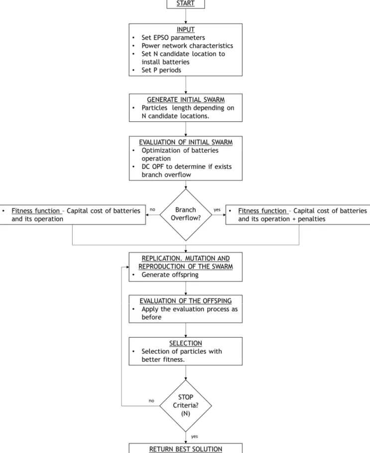
their total. This value represents the required energy imported or exported in each period, which will give us the costs/profits of placing batteries in the distribution system used. The basic operation of the EPSO method can then be seen in the scheme that follows.

In the objective function, penalties are inserted as a high cost value with the objective of penalizing particles that produce power flows that aren’t within the normal network operation. As the model operates in a DC OPF these penalties will refer to cases where maximum line power flow is surpassed. These penalties will lead to a worse value in the fitness function and has the purpose of eliminating this particles in the evaluation and selection process.

(37)

19

(38)

4.2. Battery Operation Optimization Using Linear Programming

To find the best possible scenario for sizing and location of batteries regarding active power, it is required that the best operation is found for each one of them inserted into the distribution network. This means that it is required to use an optimization model. Linear programming was the optimization selected for resolving the lower level problem (figure 4.1).

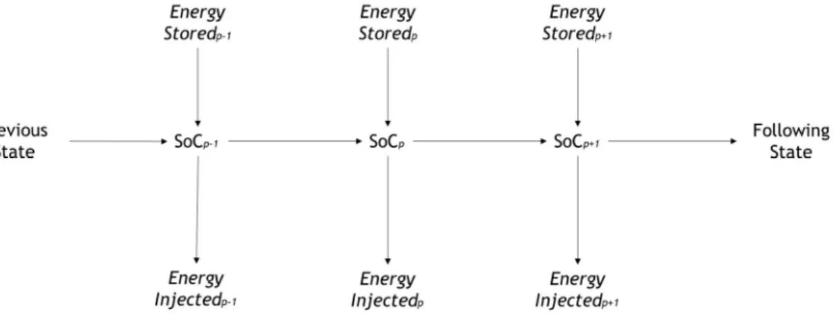
The battery operation was modelled by basing it in the operation of hydro stations as they use a similar process to store energy [4], [24],[25]. For each period, it is taken into consideration the state of charge (SoC) of the previous period, the energy that will be injected into and energy stored from the network. The scheme bellow represents how each period will interact with its adjacent periods (before and after).

This scheme can be translated into the following equations for the use of one battery over time:

𝑺𝒐𝑪_𝒑= 𝑺𝒐𝑪_{𝒑 𝟏}+ 𝒄_𝒑− 𝒅_𝒑 (4.10)

where 𝑐 represents battery charge and 𝑑 battery discharge over period 𝑝. With this representation, the modelling of the linear programming was done by applying for each battery used, the equations beneath.

𝐦𝐢𝐧 ∑𝑵𝒑 𝑪𝒐𝒔𝒕𝒑∗ (𝒄𝒑− 𝒅𝒑) (4.11)

∀_𝒑 𝒄_𝒑, 𝒅_𝒑 ≤ 𝑴 (4.12)

∀_𝒑 𝟎 ≤ 𝒄_𝒑, 𝒅_𝒑 (4.13)

∀_𝒏 𝑺𝒐𝑪 ≤ 𝑺𝒐𝑪_𝒑≤ 𝑺𝒐𝑪 (4.14)

∀𝒑 𝑺𝒐𝑪𝒑= 𝑺𝒐𝑪𝒑 𝟏+ 𝒄𝒑− 𝒅𝒑 (4.15)

(39)

21

Considering 𝑝 as the period being calculated, 𝐶𝑜𝑠𝑡 represents the price that was inserted into this period in the scenario determined previously. 𝑆𝑜𝐶 and 𝑆𝑜𝐶 represent the maximum and the minimum value of SoC, where 𝑆𝑜𝐶 is the size of the battery being optimized and 𝑆𝑜𝐶 10% of that size. 𝑀 represents the maximum value for charge or discharge at any given period.

To make a more independent model and, as was mention in the beginning of this chapter, there was created a database that includes different charge/discharge rates to acknowledge the different battery technologies existent. The value given by the upper level problem to this rate is processed in the linear programming as 𝑀. This value equals the multiplication of the charge/discharge rate taken from the particle of said battery and its size.

𝑴 = 𝜸_𝒏∗ 𝒔𝒊𝒛𝒆_𝒏 (4.16)

For each battery optimization, 𝛾 and 𝑠𝑖𝑧𝑒 will influence the behaviour of the said battery over the course of 𝑃 periods. The data of this behaviour will be transmitted into the EPSO algorithm in the form of 𝐵𝑙 , and 𝐵𝑔 , for each period. This is done for the 𝑁 possible

batteries present in the particle. With these values, EPSO will calculate the Network Operation costs that will lead to the evaluation of the particle and, therefore, the best 𝛾 and 𝑠𝑖𝑧𝑒 for each location can be found.

(40)

(41)

Chapter 5 Case Study

In this chapter, it is going to be applied the model presented in the previous ones. The tool used to do so was created in a MATLAB environment. The simulations presented were done in a modified CIGRE MV distribution benchmark network to validate the model proposed.

5.1. CIGRE MV Distribution Network Benchmark

The configuration used is the European configuration for this CIGRE network benchmark [26], with three-phase feeders, which can be either meshed or radial (figure 5.1). It operates at 20 kV in both feeder and is fed by a 110 kV subtransmission network (HVN).

The network is used in its radial configuration, where the switches S1, S2 and S3 are open. The switches that link both bus 1 and bus 12 to the bus linked to HVN are closed. The voltage is balanced along the MV lines which is a good match to the model presented, as the unbalanced voltage problem is not considered.

Lines are divided into two configurations. On feeder 1, they are underground and the cables are XLPE with round, stranded aluminium conductors and copper tape shields. Lines on feeder 2 are made from aluminium with steel reinforcement and are aerial.

All system parameters were changed into pu unities to fit the model created. The power base used to do the system transformation from the international system of units (SI) to pu is 100 MW and the voltage base is 20 kV in the distribution network and 110 kV in the HVN. The network was considered symmetric and balanced. The parameters of lines and transformers are presented (in Appendix A, table A.1) in pu units with the transformers already converted into line parameters.

(42)

24 Case Study

These values are then used to calculate the sensitivity matrix (in Appendix A, table A.2) that is used in the optimization to calculate the power flow. Load data was processed accordingly to the season load curves presented in chapter 3 and with data from CIGRE benchmark network [26]. This led to the creation of the seasons’ load data that is presented (in Appendix A, tables A.3, A.4 and A.5) There were also introduced distributed generation into the network in the form of PV generation. This generation is integrated in buses 3 to 6 and buses 8 to 11.

5.2. Stochastic Scenario Creation

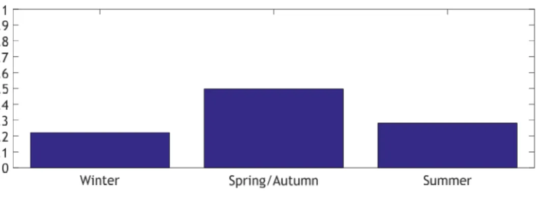
To better evaluate the model created, the following stochastic scenario was created using the information presented in chapter 3. The scenario was generated for a full year (365 days) and seasons are shown as percentage of the total of years. Winter has an occurrence of 22%, Spring/Autumn 50% and Summer 28% (figure 5.2.). This information could be interpreted as a year where hot weather was more predominant over the colder weather.

Figure 5.1: Topology of MV Distribution network benchmark

(43)

25

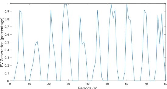
With this information, PV generation was set by multiplying the nominal PV generation of each generator by the amount of PV exploitation percentage that is given by the stochastic scenario. These values were calculated for each season accordingly to the weather condition scenario that was selected for each day. This gave to the model the value of energy produced in each period of time. The behaviour of PV generation (in percentage) for each generator for a year is illustrated in figure 5.3. As there is too much data, a graph that represents the first 10 days is presented (figure 5.4).

Figure 5.2: Seasons probabilities.

PV G en er at io n (p er ce nt ag e)

(44)

26 Case Study

By having the stochastic scenario set, load and price values are inserted into the model by selecting from the load and energy price season’s tables, presented in subchapter 5.1, the values for each representing day (figures 5.5, 5.6, 5.7 and 5.8).

PV G en er at io n (p er ce nt ag e)

Figure 5.4: PV Generation Behaviour in Bus 4 for 10 days.

Lo

ad

(

pu

)

(45)

27

Figure 5.8: Energy Prices over 10 days

Pr ic es ( pu ) Lo ad ( pu )

Figure 5.6: Load in Bus 4 over 20 days.

Pr ic es ( pu )

(46)

28 Case Study

5.3. Battery Scenarios

The batteries that were inserted in this case study, by reviewing the literature of chapter 2, are comprised between a range of 1kW to 10 MW, moreover, the battery sizing optimization problem will follow a linear perspective. This can be explained by the way that batteries are constructed. A battery is assembled by the use of smaller battery modules. This means that a battery system can be devised to be of a specific size, which does not happen in devices such as power transformers. The battery cost will then follow a linear function that depends of its size [27]. The following equation refers to battery investment costs in €/pu.

𝑩_{𝑰𝒏𝒗𝒆𝒔𝒕𝒎𝒆𝒏𝒕 𝑪𝒐𝒔𝒕} = 𝟑𝟎𝟓𝟎𝟎𝟎 ∗ 𝒔𝒊𝒛𝒆_𝒏 (5.1)

As for the power electronics, each type of technology has a different investment cost [4]. So, to represent this, 4 different charge/discharge rate were used and each of them have a different cost (table 5.1).

Table 5.1 Power Electronics Costs

Charge/Discharge Rate Power Electronics Investment Costs (€/pu)

0.3 70000

0.5 128000

0.7 180000

0.9 350000

5.4. Battery Operation

Battery operation was optimized using linear programming. As this information depends on the size of battery and its charge/discharge rate, the following results an example of the operation with SoC values as percentages and with 0.7 charge/discharge rate. The results presented are an example of what operation results are given for a battery in any given bus during the optimization process. In figure 5.9, the operation of a battery is presented for one day.

(47)

29

It is possible to see how the battery tends to discharge its charge when the price is high during a period of times. On lower price periods the battery charges. It is even possible to see that there is also present the decision of the battery holding charge, without charging or discharging due to the possibility of having a better charge/discharge compensation by doing it in later periods.

The previous graph is an example of the behaviour for a multiday operation. The battery is going to end as fully discharged to represent the cost opportunity of selling all energy at the end of the last period, which is what is inserted in the model operation. In this graph is also perceivable the different behaviour that occurs for different season days.

The operation behaviour that is presented is what EPSO requires from linear programming so that the network’s operation costs include the information for battery charge

Figure 5.9: Battery State of Charge (0.7 Charge/Discharge Rate) and Energy Price over 1 Day.

St at e of C ha rg e En er gy P ri ce ( pu ) St at e of C ha rg e En er gy P ri ce ( pu )

(48)

30 Case Study

or discharge in each period of time. This is done for all batteries with this information EPSO can calculate every power flow to determine operation costs and then finalize the evaluation required in EPSO.

This optimization model was executed previously to the EPSO routine in MATLAB. Battery SoC was considered in percentage and each type of charge/discharge rate was optimized for the stochastic scenario presented and saved into a database. This allowed for a faster execution of the EPSO optimization as, instead of using the linear programming optimization for each battery in each iteration, EPSO just needed to do a data search for the charge/discharge rate used and multiply SoC and the charge and discharge values for each period by the battery´s size.

5.5. Battery Sizes and Locations

In this subchapter, a comparison between results for different number of particles is presented. The comparison was made between 10, 20 and 50 particles and each bus from the network was a possible location except for bus 15 as this one is used as the slack bus.

Battery sizing and Location and the respective power electronics were determined for each of the 3 number of particles cases mentioned and their final results were compared.

For the 10 particles case, batteries were located in buses 3, 5, 7 11 and 12 with 0.01 pu, which translates into 1MW. As for charge/discharge rates, bus 3 has a 0.7 rate, buses 5, 7 and 11 have a 0.9 rate and bus 12 has a rate of 0.3 (figure 5.11).

Figure 5.11: Size and Charge/Discharge rate for 10 particles used in the model with 1MW maximum size

Si ze ( M W ) C ha rg e/ D is ch ar ge R at e

(49)

31

In the case where 20 particles were used, the same batteries were located in buses 3, 5, 7 and 11, where only the charge/discharge rate in bus 3 was changed from the previous 70% to 90%. New batteries were sized and located in buses 9 and 14 with the value of 0.01 pu (1MW). From comparing results with the 10 particles case, the battery located in bus 12 was changed into bus 14, which resulted in better operation costs for the network. This also made the charge/discharge rate from the feeder 2 batteries shift into lower rates (figure 5.12).

Finally, for 50 particles, batteries with size 0.01 pu were located in buses 3, 5, 7, 9, 11 and 13 and a battery with size 0.00566 pu (0.566 MW) was inserted in bus 6. Charge/discharge rates were of 0.9 for all buses except bus 9 and 13 which have 0.7 and 0.3 rates respectively (figure 5.13).

Figure 5.13: Size and Charge/Discharge rate for 50 particles used in the model with 1MW maximum size Figure 5.12: Size and Charge/Discharge rate for 20 particles used in the model with 1MW maximum size

(50)

32 Case Study

In the case where 20 particles were used, the same batteries were located in buses 3, 5, 7 and 11, where only the charge/discharge rate in bus 3 was changed from the previous 70% to 90%. New batteries were sized and located in buses 9 and 14 with the value of 0.01 pu (1MW). From comparing results with the 10 particles case, the battery located in bus 12 was changed into bus 14, which resulted in better operation costs for the network. This also made the charge/discharge rate from the feeder 2 batteries shift into lower rates (figure 5.12).

Finally, for 50 particles, batteries with size 0.01 pu were located in buses 3, 5, 7, 9, 11 and 13 and a battery with size 0.00566 pu (0.566 MW) was inserted in bus 6. Charge/discharge rates were of 0.9 for all buses except bus 9 and 13 which have 0.7 and 0.3 rates respectively (figure 5.13).

The comparison of the costs of each case is presented in the following figure.

Figure 5.15: Size and Charge/Discharge rate for 50 particles used in the model

Figure 5.14: Size and Charge/Discharge rate for 20 particles used in the model

(51)

33

By evaluating these costs evolutions, it is concluded that for the 10 and 20 particles cases, the best solution wasn’t found. This leads to assume that for these cases, a local solution was found and there wasn’t a mutation that led to a better solution. This failure to find the best solution in each one of this cases is due to the number of particles used. As the number decreases, the number of mutation done also decreases, which decreases the probability for the best solution to be found. It is also possible to see that with a larger number of particles, the optimization is done in fewer iterations of EPSO.

5.6. Different Maximum Battery’s Sizes

Most of the batteries in the cases presented were sized with the maximum size limit introduced into the program. So, to test if the sizing of each battery isn’t being optimized by this limitation, the value was changed from a maximum of 1 MW to 10 MW. In this simulation, batteries were located in the same buses, 3, 5, 7, 9, 11 and 14 and a new battery in bus 2 was introduced (figure 5.16).

In this experiment, as several runs of the program were made, it was possible to verify that the limit imposed in the previous subchapter was limiting a better solution for this network. Moreover, it is possible to see different responses to the sizing and power electronics optimization. As it can be seen in buses 2 and 11 in figure 5.15, a better power electronic solution was selected over maximum sizing, whereas in buses 5 and 7 a bigger battery was preferred over a faster charge/discharge rate. This leads to conclude that a trade-off between size and faster power electronics exists. In some locations of the network, there is a preference for the charge/discharge rate optimization and in other locations, sizing is preferred over power electronics.

Figure 5.16: Costs function evolution of each case presented.

C

os

ts

(

(52)

34 Case Study

These results also lead to the assumption that even in a scenario where it is possible to use a single larger battery to be installed in the network, the optimization is inclined to a solution with batteries dispersed over the network. These conclusions suggest that pre planning studies are required to a better solution in the battery sizing and location problem solving.

5.7. Model’s Robustness

The model implemented was tested for 30 runs for each one of the cases mentioned in 5.5. As this model is based on an iterative optimization method, the solution that is given may not be the best solution possible as the program might not mutated in the optimal way to find, in

Figure 5.17: Optimization for the 10MW maximum size case. Figure 5.18: Costs function evolution of the maximum 10MW size case

(53)

35

the amount of iterations done, the optimal solution. In this subchapter the comparison between the dispersal of results for the 30 runs for each case is done.

The results of the runs made are presented below. Here it is possible to see that, for a numerous particles case, the dispersion of results is lower. This is explained by the amount of mutations that are done by having a larger swarm. With more particles there is also more probability that one of them finds the best solution within the limit of iterations.

The dispersal of results was calculated by translating the results from their real values to percentages, where the solution’s cost was divided by the best solution of each case. Then, the following equation was used to determine how much the solutions found stray from the best one in percentage: 𝑫𝒊𝒔𝒑𝒆𝒓𝒔𝒂𝒍_{𝒄𝒂𝒔𝒆}=∑ (𝑺𝒐𝒍𝒖𝒕𝒊𝒐𝒏𝑺𝒔 𝒔 𝑩𝒆𝒔𝒕 𝑺𝒐𝒍𝒖𝒕𝒊𝒐𝒏) 𝑺 𝟏 ( 5.2) C os ts (€ )

Figure 5.20: Solutions using 10 particles in the model's optimization.

C

os

ts

(€

)

(54)

36 Case Study

The dispersal results are presented in the following table.

Table 5.2: Dispersal results for each case.

10 Particles 20 Particles 50 Particles

11.98% 6.16% 3.87%

These values lead to conclude what was already assumed previously. With a larger number of particles, the value given from a single run of the program is optimized by using more particles in the optimization. This also leads to the conclusion that the model presented is, in fact, capable of obtaining a good solution for the 50 particles case. This case is the one that is proposed to be used for further works. The value of this dispersal will also decrease if the assumptions made to simplify the problem are studied to turn the model more complex.

C

os

ts

(€

)

(55)

Chapter 6 Conclusions

6.1. Assessment from the work developed

This thesis work has allied one to reach the following implementation achievement:

1. A comprehensive enough modelling of the operation conditions of a distribution network with distributed PV generation, including the representation of stochastic uncertainties in load, energy prices and weather conditions impacting the available solar power.

2. A hybrid optimization model in a mixed-integer program formulation, where an EPSO algorithm defined integer variables (location, size of batteries, type of connection technology) at an upper level and a linear programming formulation defined optimized operation costs for the configuration proposed from the upper level, based on a DC modelling of power flows and a multiperiod optimization.

Tests were run in a realistic CIGRE distribution network and using real data on solar power, energy process and load curves. Although with a scope limited to the system tested, some interesting conclusions could be drawn:

1. Distributed solutions for battery location were privileged by the optimization process over concentrated solutions. This reinforces the notion that optimization is a required tool to design distribution systems with storage, instead of imagining that they could just be installed in the distribution substations.

2. Also, battery locations were selected dispersed in the network, and not at the extreme consumer nodes only, which suggests that distributed storage may have a competing edge over home storage, opening a feasible business option for distribution companies. 3. A trade-off between power electronics technology and battery size was detected, i.e., between storage speed and storage capacity, revealing that a portfolio of options may be available for distribution companies and therefore solutions must be comprehensively studied.

(56)

38 Conclusions

These conclusions were drawn based only on energy-related operation costs. No modelling of other advantages associated with the existence of storage have been taken in account - for instance, using the stored energy to gain business as a supplier of ancillary services to the upper voltage level operator or to improve reliability indices at the distribution level (emergency power, for instance, instead of load disconnection).

Therefore, the thesis work, by developing and implementing a suitable suite of algorithms and producing a realistic simulation over realistic data, reinforces the notion that distributed storage is a viable option for distribution networks and should be dealt with hybrid models, describing and representing the complex and stochastic reality surrounding the distribution/generation/storage environment.

6.2. Future Works

The work developed over this thesis contributes to the study of the sizing, location and operation optimization of batteries, connecting the three problems into the optimization. However, there are still new contributions to be made into the model presented to have a better performance. Some suggestions will be presented to further develop this work:

1. The model created adopted a DC OPF approach. The optimization problem would be a lot more accurate if an AC OPF was used. Also, by using AC OPF, the voltage stabilization problem could also be inserted in the model.

2. The stochastic scenarios used to simulate the operation of the grid over a year made it possible to prove this model. The use of a stochastic model with an hourly period would become more accurate. This was not done as it would require more computational processing power. There is also the possibility to use a prediction model for the system operation which would give a more realistic behaviour of the network.

3. The insertion of other types of distributed generation would insert another type of variables into the model, which would generate a completely different power flow, turning the power flows of the networks and possibly changing the sizing of the storage systems.

4. The use of a more complex optimization tool in the battery operation could also give a more accurate response of the model to the energy generation fluctuations. This would require an alteration to the model’s structure but that would be possible as EPSO and Linear programming only exchange size, charge/discharge rate and battery operation. 5. The inclusion of other business models contributing to the valorisation of storage, such as revenue resulting from ancillary services provided to transmission system operators, load management value resulting from replacing Demand Side Management options by use-of-storage options or reliability worth resulting from a reduction in load curtailment or interruption duration from resorting to storage as an alternative supply source.

(57)

Appendix A

Table A.1 Network’s line parameters.

Line Number From Node To Node R X B

1 1 2 0.5048 0.0987 0.0987 2 2 3 0.7912 0.0987 0.0987 3 3 4 0.1092 0.0987 0.0987 4 4 5 0.1002 0.0987 0.0987 5 5 6 0.2757 0.0987 0.0987 6 7 8 0.2989 0.0987 0.0987 7 8 9 0.0573 0.0987 0.0987 8 9 10 0.1378 0.0987 0.0987 9 10 11 0.0591 0.0987 0.0987 10 3 8 0.2327 0.0987 0.0987 11 12 13 0.4474 0.0603 0.0603 12 13 14 0.2736 0.0603 0.0603 13 15 1 0.4800 0.2501 0.2501 14 15 12 0.4800 0.2501 0.2501

Table A.2 Network sensitivity matrix

Bus 1 Bus 2 Bus 3 Bus 4 Bus 5

Line 1 -5.62E-16 -1 -1 -1 -1 Line 2 0 0 -1 -1 -1 Line 3 0 0 0 -1 -1 Line 4 0 0 0 0 -1 Line 5 0 0 0 0 0 Line 6 0 0 0 0 0

Line 7 -1.687E-15 -2.249E-15 -2.249E-15 -2.249E-15 -2.249E-15 Line 8 1.125E-15 1.125E-15 1.125E-15 1.125E-15 1.125E-15 Line 9 -1.125E-15 -1.125E-15 -1.125E-15 -1.125E-15 -1.125E-15

(58)

40 Appendix A

Line 11 0 0 0 0 0

Line 12 0 0 0 0 0

Line 13 -1 -1 -1 -1 -1

Line 14 0 0 0 0 0

Line 1 -1 -1 -1 -1 -1

Line 2 -1 -1 -1 -1 -1

Line 3 -1 0 0 0 0

Line 4 -1 -5.623E-16 -5.623E-16 -5.623E-16 -5.623E-16

Line 5 -1 0 0 0 0

Line 6 0 1 -1.125E-15 -1.125E-15 -1.125E-15

Line 7 -2.249E-15 -2.249E-15 -2.249E-15 -1 -1

Line 8 1.125E-15 1.125E-15 1.125E-15 1.125E-15 -1

Line 9 -1.125E-15 -1.125E-15 -1.125E-15 -1.125E-15 -1.125E-15

Line 10 0 -1 -1 -1 -1

Line 11 0 0 0 0 0

Line 12 0 0 0 0 0

Line 13 -1 -1 -1 -1 -1

Line 14 0 0 0 0 0

Line 1 -1 0 0 0 0 Line 2 -1 0 0 0 0 Line 3 0 0 0 0 0 Line 4 -5.623E-16 0 0 0 0 Line 5 0 0 0 0 0 Line 6 -1.125E-15 0 0 0 0 Line 7 -1 0 0 0 0 Line 8 -1 0 0 0 0 Line 9 -1 0 0 0 0 Line 10 -1 0 0 0 0 Line 11 0 0 -1 -1 0 Line 12 0 0 0 -1 0 Line 13 -1 0 0 0 0 Line 14 0 -1 -1 -1 0

Table A.3: Winter's Load Data

Period 1 Period 2 Period 3 Period 4 Period 5 Period 6 Period 7 Period 8 Bus 1 0.02704 0.02579 0.04053 0.04682 0.04336 0.05119 0.06118 0.04776

(59)

41 Bus 3 0.00068 0.00066 0.00107 0.00132 0.00121 0.00133 0.00144 0.00113 Bus 4 0.00060 0.00055 0.00084 0.00088 0.00082 0.00107 0.00144 0.00112 Bus 5 0.00101 0.00093 0.00141 0.00149 0.00139 0.00181 0.00243 0.00189 Bus 6 0.00076 0.00070 0.00107 0.00112 0.00105 0.00136 0.00183 0.00143 Bus 7 0.00010 0.00011 0.00018 0.00026 0.00023 0.00022 0.00018 0.00014 Bus 8 0.00081 0.00075 0.00114 0.00120 0.00112 0.00146 0.00196 0.00153 Bus 9 0.00075 0.00079 0.00135 0.00191 0.00175 0.00164 0.00133 0.00104 Bus 10 0.00075 0.00070 0.00108 0.00120 0.00111 0.00138 0.00174 0.00136 Bus 11 0.00046 0.00042 0.00064 0.00067 0.00063 0.00082 0.00110 0.00086 Bus 12 0.02726 0.02603 0.04094 0.04739 0.04388 0.05168 0.06157 0.04807 Bus 13 0.00004 0.00005 0.00008 0.00011 0.00010 0.00010 0.00008 0.00006 Bus 14 0.00072 0.00072 0.00119 0.00153 0.00141 0.00147 0.00146 0.00114 Bus 15 0 0 0 0 0 0 0 0

Table A.4: Spring/Autumn's Load Data

Period 1 Period 2 Period 3 Period 4 Period 5 Period 6 Period 7 Period 8 Bus 1 0.02496 0.02362 0.03353 0.03956 0.03990 0.03681 0.05050 0.04252 Bus 2 0 0 0 0 0 0 0 0 Bus 3 0.00066 0.00061 0.00081 0.00105 0.00113 0.00104 0.00122 0.00108 Bus 4 0.00051 0.00050 0.00077 0.00081 0.00074 0.00069 0.00115 0.00092 Bus 5 0.00087 0.00084 0.00130 0.00137 0.00125 0.00116 0.00194 0.00154 Bus 6 0.00065 0.00063 0.00098 0.00103 0.00094 0.00088 0.00147 0.00116 Bus 7 0.00011 0.00010 0.00011 0.00018 0.00022 0.00020 0.00016 0.00017 Bus 8 0.00070 0.00068 0.00105 0.00110 0.00101 0.00094 0.00157 0.00124 Bus 9 0.00084 0.00075 0.00080 0.00135 0.00168 0.00152 0.00123 0.00127 Bus 10 0.00067 0.00064 0.00094 0.00105 0.00101 0.00094 0.00142 0.00116 Bus 11 0.00039 0.00038 0.00059 0.00062 0.00056 0.00053 0.00088 0.00070 Bus 12 0.02522 0.02385 0.03377 0.03996 0.04040 0.03727 0.05087 0.04290 Bus 13 0.00005 0.00004 0.00005 0.00008 0.00010 0.00009 0.00007 0.00008 Bus 14 0.00073 0.00067 0.00084 0.00117 0.00133 0.00121 0.00127 0.00118 Bus 15 0 0 0 0 0 0 0 0

Table A.5: Summer's Load Data

Period 1 Period 2 Period 3 Period 4 Period 5 Period 6 Period 7 Period 8 Bus 1 0.03065 0.02853 0.03538 0.04501 0.04675 0.04553 0.04606 0.03970 Bus 2 0 0 0 0 0 0 0 0 Bus 3 0.00082 0.00076 0.00091 0.00119 0.00126 0.00129 0.00122 0.00109 Bus 4 0.00062 0.00058 0.00076 0.00093 0.00093 0.00085 0.00094 0.00078 Bus 5 0.00104 0.00098 0.00128 0.00156 0.00157 0.00144 0.00159 0.00131 Bus 6 0.00078 0.00074 0.00096 0.00118 0.00119 0.00108 0.00119 0.00099 Bus 7 0.00015 0.00013 0.00014 0.00020 0.00023 0.00025 0.00021 0.00020

(60)

42 Appendix A Bus 8 0.00084 0.00079 0.00103 0.00126 0.00127 0.00116 0.00128 0.00106 Bus 9 0.00109 0.00098 0.00107 0.00151 0.00169 0.00188 0.00158 0.00149 Bus 10 0.00081 0.00076 0.00096 0.00120 0.00123 0.00116 0.00122 0.00104 Bus 11 0.00047 0.00045 0.00058 0.00071 0.00071 0.00065 0.00072 0.00060 Bus 12 0.03098 0.02883 0.03570 0.04546 0.04725 0.04610 0.04653 0.04014 Bus 13 0.00006 0.00006 0.00006 0.00009 0.00010 0.00011 0.00009 0.00009 Bus 14 0.00093 0.00085 0.00098 0.00132 0.00143 0.00150 0.00137 0.00124 Bus 15 0 0 0 0 0 0 0 0

Table A.6: PV Generation

PV Nominal Generation (kW\h) PV Nominal Generation (pu)

Bus 3 300 0.003 Bus 4 300 0.003 Bus 5 400 0.004 Bus 6 400 0.004 Bus 8 400 0.004 Bus 9 400 0.004 Bus 10 500 0.005 Bus 11 200 0.002

BASSILO - Battery storage sizing and location in distribution systems

Faculdade de Engenharia da Universidade do Porto

BASSILO

Battery storage sizing and location in distribution

systems

Tiago João Amorim Abreu

Mestrado Integrado em Engenharia Eletrotécnica e de Computadores

Major Energia

Supervisor: Vladimiro Miranda (Full Professor)

Resumo

Abstract

Acknowledgements

Contents

Resumo ... v

Abstract ... vii

Acknowledments ... ix

Contents ... vi

List of figures ... xiii

List of tables ... xv

Abbreviations and Symbols ... xvii

Chapter 1 ... 1

Chapter 2 ... 3

Chapter 3 ... 11

Chapter 4 ... 15

Chapter 5 ... 23

Chapter 6 ... 37

Appendix A ... 39

List of figures

List of tables

Abbreviations and Symbols

Chapter 1

Introduction

Chapter 2

State of Art