Lat. Am. j. solids struct. vol.13 número2

(1)

Abstract

The global optimization of integer and mixed integer non-linear problems has a lot of applications in engineering. In this paper a heuristic algorithm is developed using line-up competition and gen-eralized pattern search to solve integer and mixed integer non-linear optimization problems subjected to various linear or nonlinear con-straints. Due to its ability to find more than one local or global optimal points, the proposed algorithm is more beneficial for multi-modal problems. The performance of this algorithm is demonstrated through several non-convex integer and mixed integer optimization problems exhibiting good agreement with those reported in the lit-erature. In addition, the convergence time is compared with LCAs’ one demonstrating the efficiency and speed of the algorithm. Mean-while, the constraints are satisfied after passing only a few itera-tions.

Keywords

Global optimization, integer optimization, mixed integer optimiza-tion, multi-modal problems, constraint optimization.

A Heuristic Algorithm Based on Line-up Competition

and Generalized Pattern Search for Solving Integer and Mixed

Integer Non-linear Optimization Problems

1 INTRODUCTION

A vast number of optimization problems deal with integer variables. Due to the complexity of either the objective function or the constraints, these problems can be a real challenge. The presence of nonlinearities in the objective and constraint functions might imply non-convexity in mixed integer

Behrooz Shahriari a* M. R. Karamooz Ravari b Shahram Yousefi c Mahdi Tajdari d

a,c _{Department of Mechanical and}

Aerospace Engineering, Malek-Ashtar University of Technology, Isfahan,

84145-115, Iran.

b _{Department of Mechanical Engineering,}

Graduate University of Advanced Technology, Kerman, 76311-33131, Iran. d _{Department of Mechanical Engineering,}

Islamic Azad University, Arak Branch,

Arak, Iran.

Corresponding author email: * shahriari@mut-es.ac.ir

http://dx.doi.org/10.1590/1679-78252293

(2)

Latin American Journal of Solids and Structures 13 (2016) 224-242 nonlinear programming (MINLP) problems, i.e. the potential existence of multiple local solutions. A mixed integer optimization problem can be formulated as:

min ( )

(x) 0 1,...,

1,...,

1, .

... :

,

i j

k

r r r

f

g i p

h j q

x R k s

x Z k s n

l x u r n

S T

£ =

= =

Î =

Î = +

£ £ =

x

where n is the number of variables, x is the vector of variables, and ( ,l u_r _r)are the boundaries of the variable xr.

The solution methods are classified into three major classes and named as: relaxation methods, search heuristics, and pattern search methods (Abramson, 2002).

Relaxation methods such as outer approximation(Duran and Grossman, 1986; Fletcher and Leyffer, 1994), generalized bender decomposition(Geoffrion, 1972), branch and bound methods (Dakin, 1965; Leyffer, 1998; Kesavan and Barton, 2000), and extended cutting plane (Kelley, 1960; Marchand et al., 2002; Wang, 2009), involve solving several sub-problems. The solution process needs the linearization of some sub-problems which requires cost function and constraints to be differentiable.

Search heuristics are methods designed to find global optima without using derivative information by systematically searching the solution space (Abramson, 2002). These methods often are based on the principles of natural biological evolution. The most relevant algorithms to solve MINLP are sim-ulated annealing (Gidas, 1985), Tabu search (Glover, 1990; Glover, 1994), and evolutionary algo-rithms such as Genetic Algorithm (Holland, 1962; Costa and Oliveira, 2001; Deep et al., 2009), Evo-lutionary Strategy (Costa and Oliveira, 2001), EvoEvo-lutionary Programming (Fogel et al., 1966), Ant Colony Optimization (Schluter et al., 2009), Particle Swarm Optimization (Coelho, 2009), and Dif-ferential Evolution (Ponsich and Coello, 2009; Lin et al., 2004).

Pattern search methods were proposed to minimize a continuous function without any knowledge of its derivative. The class of generalized pattern search (GPS) methods was introduced for solving unconstrained non-linear programming (Box, 1975), and was used to optimize mixed integer con-straint non-linear optimization problems (Audet and Dennis, 2001).

The line-up competition algorithm (LCA) which is categorized in evolutionary algorithms was pro-posed to optimize non-linear (Yan and Ma, 2001) and mixed integer non-linear optimization problems (Yan et al., 2004).

(3)

Latin American Journal of Solids and Structures 13 (2016) 224-242

2. ALGORITHM

This section of the paper is allocated to the description of the proposed algorithm. First, in subsection 2.1,an overall perspective of the algorithm is presented, and the steps which should be followed are explained. In subsections 2.2 to 2.7, these steps are mathematically formulated and their details are discussed.

2.1. Outline on the Present Algorithm

In the present algorithm, a uniform mesh is first generated over the solution space as the initial population. This uniform mesh guarantees that the initial population covers the whole search space not leading to loss any area of the space. In the rest of the paper, each point of the mesh is called a "family". These families are ranked to form a line-up according to the values of their objective func-tions, i.e. the best family is placed in the first position in the line-up, while the worst is placed in the final position. Based on the position of each family in the line-up, a search space is allocated to each family. In the next step each family produces 2n children in its allocated search space, where n is the number of variables. These children are produced using generalized pattern search method which cause that all the directions on the corresponding search space get covered. The members of each family compete with each other, as well as their father, and the best one survives as the father of the next generation. This algorithm can be described as follow:

1. Generate mesh points on the search space and compute the value of the objective function for each family.

2. Rank the mesh points to form a line-up according to their objective function values. For a minimization problem the line-up is an ascending sequence and vice versa.

3. Allocate a search space to each family according to their position in the line-up. The best family (first in the up) has the smallest search space, while the worst (final in the line-up) has the biggest search space.

4. Produce 2n children using generalized pattern search method. Then, the children compete with each other, as well as their father, and the best one survives as the next generation's father.

5. Update the search space according to the f-th first family. The search space will be expanded if there is at least one improvement in the f-th first family and will be contracted if there is no improvement in the f-th first family. Notice that the value off is defined by the user and helps to find more than one optimal point.

6. If the stopping criterion isn’t satisfied return to (3).

The above-mentioned steps are described in mathematical terms in the following subsections.

2.2. Mesh Generation

(4)

Latin American Journal of Solids and Structures 13 (2016) 224-242 Let’s define vector m, whose arrays, m1 to mn, denote the number of mesh points which should be

generated in ( ,l u₁ ₁) to ( ,l u_n _n), respectively. The mesh points related to mj are generated in( ,l u_j _j) utilizing the following equation.

j j

1

( ) j 1,...,s ,t 1,...,m 1

1

[ ( )] j 1,...,n ,t 1,...,m 1

j

jt j j

j j

jt j j

j

t X l

m t

X INT l s

m

ì

-ïï ₌ ₊ _D ₌ ₌

ïï

-ïï

íï

-ïï = + D = + =

ïï

-ïî

(1)

whereD =_j u_j -l_j,

j jt

X is the t_j-th value in ( ,l u_j _j), and INT denotes the integer operator. Notice

that mj-s control the number of mesh points.

A matrix, M, containing the mesh points is defined, which has n rows and C columns where Cis calculated as: 1 n r r C m =

=



(2)

Each column of M denotes a mesh point in the search space. The arrays of this matrix (mip) are

generated using Eq.3.

1

1 1

i i

i-1 i-1

q q

q 1 1 q 1 1

i

( 1)

1 and 1

(a -1)C ( 1) (a -1)C

1 and i 1

m m

p 1,...,C ,t 1,...,m ,i 1,...n

t

ip

it _i _i

q q

t C tC

X if p i

m m

t C tC

M

X if p

m m

= = = =

ì

-ïï _{+ £ £} ₌

ïï ïï

ïï

-= í ₊ _{+ £ £} ₊ _>

ïï ïï ïï ïïî

= = =



(3)

in which 1 1 1,..., i i q q a m -=

=



. Figure 1 shows the generated mesh for n=3, m=[3 2 3]T, l=[0 2 1]T, and

u=[1 4 10]T, with the use of Eq. 3.

(5)

Latin American Journal of Solids and Structures 13 (2016) 224-242 The mesh matrix, M, for this example is as follow:

0 0 0 0.5 0.5 0.5 1 1 1 0 0 0 0.5 0.5 0.5 1 1 1

2 2 2 2 2 2 2 2 2 4 4 4 4 4 4 4 4 4

1 6 10 1 6 10 1 6 10 1 6 10 1 6 10 1 6 10

é ù

ê ú

= ê ú

ê ú

ë û

M

2.3. Ranking the Families

The columns of the mesh matrix, M, should be ranked based on their objective function values. ConsideringW= êé_ëw₁ w₂ ... w_cù_ú_û as a vector, whose arrays are the ranked objective function

val-ues, V would be a matrix where its columns are the mesh points corresponding to the arrays of W.

2.4. Allocation of the Search Space

Allocation of the search space is based on the position of each family in the line-up. In other words, the best family has the smallest search space and the worst has the biggest one. The search space for the j-th mesh point is a rectangular region. The lower and upper boundaries of i-th variable for j-th family (mesh point) in k-th generation are calculated using Eq. 4 and Eq. 5, respectively:

( )

( ) ( )

( )

( ) ( )

max , i 1,...,s ,j 1,...,C 2

max , i 1,...,n

2

k

k k i

ij ij i

k

k k i

ij ij i

j

L V l

C

j

L INT V l s

C ææ _{D ⋅ ÷ ÷}ö ö

çç _{÷ ÷}

çç

= _çç_çç - ÷ ÷_{÷ ÷} = =

÷ ÷ çç

èè ø ø

é ææ_çç _{D ⋅ ÷ ÷}ö öù

ê çç ÷ ÷ú

= _ê _çç_çç - ÷ ÷_{÷ ÷}_ú = +

÷ ÷ çç

ê èè ø øú

ë û

,j=1,...,C

(4)

( )

( ) ( )

( )

( ) ( )

min , i 1,...,s ,j 1,...,C 2

min , i 1,...,n

2

k

k k i

ij ij i

k

k k i

ij ij i

j

U V u

C

j

U INT V u s

C ææ _{D ⋅ ÷}ö ö_÷

çç _÷ _÷

çç

= _çç_çç + ÷_÷ ÷_÷ = =

÷ ÷ çç

èè ø ø

é ææ_çç _{D ⋅ ÷}ö öù_÷

ê çç ÷ ÷ú

= _ê _çç_çç + ÷_÷ ÷_÷_ú = +

÷ ÷ çç

ê èè ø øú

ë û

,j=1,...,C

(5)

2.5. Production of Children

In each family 2n children are produced utilizing GPS(2n). Let’s define children generator matrix, D, as follow:

D= êé_ëI_n -I_nù_ú_û ₍₆₎

where In is unit matrix. Now, the arrays of the children matrix of s-th family in k-th generation are

produced using the following equation:

( , ) 0 1 1 is ij s k

ij is ij

is ij

V D

CH L D

U D

ìï =

ïïï

=_íï =

-ï ₌

ïïî

(6)

Latin American Journal of Solids and Structures 13 (2016) 224-242 After generating the children, they compete with each other and their father. The winner of the competition will be the father of that family for the next generation. Notice, that if the father wins in the competition, he again stands as the father of the next generation. But, if one of the children wins the competition, the father will be replaced by the best child.

2.6. Update the Search Space

The search space will be expanded if there is at least one improvement in the f-th first family as:

(

)

(k 1) _min ( )k _, _j _1,...,n

j a j j

+

D = D D = ₍₈₎

where ̝ is the expansion factor and ̝>1.The search space will be contracted if there is no improve-ment in the f-th first family as:

( 1) ( )

j 1,...,n

k k

j b j

+

D = D = (9)

where ̞ is the contraction factor and 0<̞<1.

2.7. Stopping Criterion

The stopping criterion can be explained by Eq.10:

( )

1 2

( )

k

k f k

best

and Max V X

e e

D

< < ₍₁₀₎

where Max V

( )

_f( )k is the maximum constraint violation of the f-th first family, ε1 is the convergence

tolerance parameter, and ε2 is constraint violation tolerance.

3. IMPLEMENTATION

3.1. Constraint Handling

Constraint handling in optimization problems is a real challenge. In this paper, a pseudo cost function approach is used to replace the original objective function with a pseudo cost function, which is a weighted sum of the original objective function and the constraint violations (Vanderplaats, 1999). Therefore, the pseudo cost function acts as the objective function of the new unconstrained optimi-zation problem. Eq. 11 shows the mathematical explanation of a classical pseudo cost (static penalty function (Back et al., 1997)) function.

(

)

(

)

(

)

(

1 2 ... p max 0, 1 max 0, 2 ... max 0, m

)

F = f +P h + h + + h + g + g + + g ₍₁₁₎

(7)

3.2. Algorithm Parameters Choice

There are several parameters in the present algorithm which should be chosen by the user. It is important to use appropriate values for these parameters because they influence the performance of the algorithm. These parameters are vector m, expansion factor _̝, contraction factor _̞, f (as described previously), penalty factor p, and stopping criterion tolerances ε1 and ε2.

The larger value for the arrays of m makes it possible to find the global optimum point more accurately. However, it increases the computational time. It’s suitable to choose the value of its arrays according to the optimization cost function, constraints, and boundaries. In other words, for highly non-linear problems, the arrays of m might be increased. Also, for a wide boundary of the j-th vari-able, a larger value for mj is suitable. In this paper mj=2 is used for all examples except example 12,

and the obtained results are winsome, so mj=2 seems suitable, but in problems with lots of variables,

e.g. example 12 mj=1 can be used.

Expansion and contraction factors influence the quality of the solution and computational time. A larger value for both expansion and contraction factors provides better results, but the computa-tional time increases. Meanwhile, larger values for provide better global search. Based on our com-puting experiences, for a simple problem, ≥ 0.4 is sufficient for finding the global optimal solution. While for a difficult problem, ≥ 0.9 is recommended. For both simple and difficult problems, ̝=1 is efficient. Note that the word “simple” refers to problems with a small number of local and global minima, while the word “difficult” refers to noisy problems with several local and global minima. In other words, if there are several minima in the solution space, a small value of ̞ will cause a fast contraction of the search space leading to the loss of some optima.

A larger quantity for thef parameter provides a better global search and helps to find several global and local optimal points (if they exist), but the time of convergence to a global solution is possibly much longer. So, the value of this parameter might be chosen according to the non-linearity of the cost function and constraints.

Penalty factor is another important parameter which can affect the performance of the algorithm. The value of this parameter should be large enough in comparison with the cost function value. A value about 1010 times greater than the values of the cost function is suitable for this parameter. In addition, when there are several constraints with a different order of magnitudes, all the constraints should be normalized.

Smaller stopping criterion tolerances make the convergence slow and their choice depends on the desired precision.

4. NUMERICAL RESULTS

(8)

Latin American Journal of Solids and Structures 13 (2016) 224-242 ̝ ̞ f ε1 ε2 P(penalty factor)

Example 1 1 0.4 8 10-4 10-6 1010 Example 2 1 0.4 8 10-4 ₁₀-6 ₁₀10

Example 3 1 0.9 10 10-3 10-6 104 Example 4 1 0.9 10 1 10-6 unconstraint Example 5 1 0.85 10 1 10-6 _unconstraint

Example 6 1 0.85 10 1 10-6 109 Example 7 1 0.95 10 1 10-6 109 Example 8 1 0.96 8 0.01 10-6 _unconstraint

Example 9 1 0.95 10 10-3 10-6 109 Example 10 1 0.95 10 1 10-6 109 Example 11 1 0.95 10 10-3 10-6 109 Example 12 1 0.97 10 10-3 ₁₀-8 ₁₀20 Table 1:Algorithm parameters for each example.

Example 1: This example is taken from (Yan et al., 2004) and also given in (Costa and Oliveira, 2001; Deep et al., 2009).

{ }

2

3 1

1 2

2 3

1 3

1

2

3

min (x) 0.7 5( 0.5) 0.8

exp( 0.2) 0

1.1 1

1.2 0.2

0.2 1

2.22554 1

0,1 . :

f x x

x x

x

x S

x T

= - + - +

- - - £

+ £

-- £

£ £

- £ £

-Î

The global optimum point is x_opt =_ëé_ê0.9419 -2.1 1_û_úù withf(x_opt)= 1.0765. The result is in

full agreement with other studies. Figure 2 (a) and (b) show the history of pseudo cost function value and convergence parameter, respectively. Referring to this figure, a fast convergence to the global optimal point is achieved.

(a) (b)

(9)

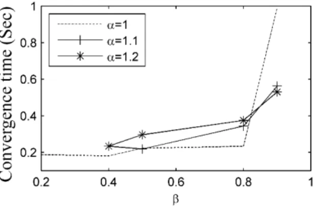
Figure 3 shows the variation of the convergence time with parameter ̝ for several values of ̞. According to this figure, ̝=1 and ̞=0.4 are the best values for fast convergence to the optimal point.

Figure 3: Example 1, convergence time vs. ̞ for three values of ̝.

Example 2: This example is taken from (Yan et al., 2004).

2 2 2 2 2 2

1 2 3 4 5 6 7

min (x) ( 1) ( 2) ( 3) ( 1) ( 2) (

.

1) l 1

:

n( )

f x x x x

S

x x x

T

= - + - + - + - + - + - - +

1 2 3 4 5 6 5

x +x +x +x +x +x £

2 2 2 2

1 2 3 6 5.5

x +x +x +x £

1 4 1.2

x +x £

2 5 1.8

x +x £

3 6 2.5

x +x £

1 7 1.2

x +x £

2 2

2 5 1.64

x +x £

2 2

3 6 4.25

x +x £

2 2

3 5 4.64

x +x £

0 1,2, 3

i

x ³ i =

{ }

0,1 4,..., 7 i

x Î i =

The global optimum point is x_opt = ê_ëé0.2 0.8 1.9079 1 1 0 1ù_ú_ûTwithf(x_opt)= 4.5796. The

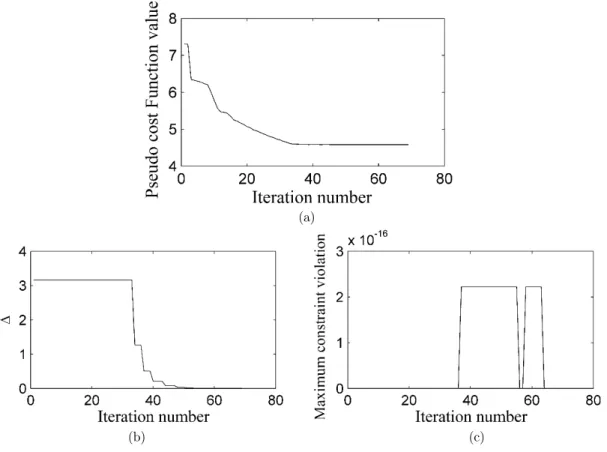
obtained optimum point is in full agreement with that reported in(Yan et al., 2004). The pseudo cost function, convergence parameter, and maximum constraint violation history of the problem are de-picted in figure 4 (a)-(c), respectively, showing fast convergence to the optimum point. The maximum constraints violation is almost zero in all iterations, meaning that the generated mesh covers the search space appropriately.

Figure 5 compares the convergence time for several values of ̝ and ̞. Referring to this figure,

(10)

(a)

(b) (c)

Figure 4:Example 2, (a) pseudo cost function history, (b) Convergence parameter history, (c) Maximum constraint violation history.

Figure 5:Example 2, convergence time vs. ̞ for three values of ̝.

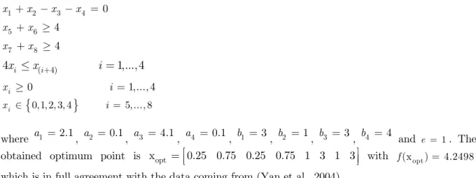
Example 3: This is a synthesis problem of a process system, taken from (Yan et al., 2004).

4

( 4) 1

min (x) ( exp( ) ln(

. :

11 ))

i i i i

i

f a x b x

S T

+ =

=

å

-1 2

(11)

1 2 3 4 0

x +x -x -x =

5 6 4

x +x ³

7 8 4

x +x ³

( 4)

4x_i £x_i₊ i =1,...,4

0 1,..., 4

i

x ³ i =

{

0,1, 2, 3, 4

}

5,..., 8 i

x Î i =

where a1 =2.1_,a2 = 0.1_,a3 =4.1_,a4 =0.1_,b1 = 3_,b2 =1_,b3 =3_,b4 = 4_and_e ₌ ₁_{. The}

obtained optimum point is x_opt = ê_ëé0.25 0.75 0.25 0.75 1 3 1 3ù_ú_û with f(x_opt)= 4.2498

which is in full agreement with the data coming from (Yan et al., 2004).

Figure 6 (a)-(c) show the pseudo cost function, convergence parameter, maximum constraint violation history of the problem, respectively. Since there are 2 equal constraints, finding the feasible region would require that some iterations to be passed. Accordingly, all the constraints are satisfied after 26 iterations.

(a)

(b) (c)

(12)

Example 4: This example is taken from (Tian et al., 1998).

2

2 3 3

1 1 2 2 3 4

2

( 2.5)

min (x) ( 3) cos( . ) ( 6)sin( . ) ( 2) exp(

.

2 :

) 4

x

f x x x x x x

x S T

p

-= - + - + + +

-+

{

0,1, 2,..., 60

}

1,..., 4 i

T -3183.9955

Table 2: Example 4 optimal points.

(a) (b)

(13)

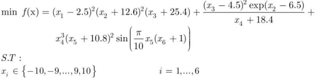
Example 5: This example is taken from (Tian et al., 1998).

2

2 2 3 2

1 2 3

4

3 2

4 5 5 6

( 4.5) exp( 6.5) min (x) ( 2.5) ( 12.6) ( 25.4)

18.4

( 10.8) sin ( )

0 :

1 1

.

x x

f x x x

x

x x x x

S T

p

-

-= - + + + +

+

æ _ö÷

ç

+ ç_ç + ÷_÷_÷

è ø

{

10, 9,..., 9,10

}

1,..., 6 i

x Î - - i =

This problem contains many global and local optimum points, of which 6 are found after only 45 iterations (Figure 8). Table 3 presents the optimal points and their values.

(a) (b)

Figure 8:Example 5, (a) pseudo cost function history, (b) Convergence parameter history.

Optimum point Optimum

value

Optimum point 1 é_ê_ë3 -10 -10 10 9 -6ù_ú_ûT -392013.974

Optimum point 2 é_ê_ë2 -10 -10 10 9 -6ù_ú_ûT -392013.974

Optimum point 3 é_ê_ë2 -10 -10 -10 9 4ù_ú_ûT -392013.974

Optimum point 4 é_ë_ê-1 -10 -10 10 9 -6ù_ú_ûT -390764.726

Optimum point 5 é_ë_ê3 -10 -10 -10 9 -7ù_ú_ûT -372826.1706

Optimum point 6 é_ë_ê2 -10 -10 -10 9 -7ù_ú_ûT -372826.1706

Table 3: Example 5 optimal points.

Example 6: This example is taken from (Costa and Oliveira, 2001) and also reported in (Deep et al., 2009).

2

1 3 4 4

max (x) 5.357854 0.835689 37.29329 40792.141

. :

f x x x x

S T

(14)

3 5 2 4 1 3

85.334407+0.0056858x x +0.0006262x x -0.0022053x x £92

2

3 5 4 5 1

80.51249+ 0.0071317x x + 0.0029955x x + 0.0021813x £110

1 3 1 4 1 2

9.300961+0.0047026x x +0.0012547x x +0.0019085x x £25

27£x_i £ 45 i =1,2, 3

{

}

4 78, 79, ,102

x Î 

{

}

5 33, 34, , 45

x Î 

The global optimum isx₁ =27,x₄ =78 for any combination of x₂and x₅. The optimum point is obtained after only 2 iterations which exhibits fast convergence.

Example 7: This example is taken from (Deep et al., 2009).

1 7 2 6 3 5 4

min (x)f =x x +3x x +x x +7x

1 2 3 6

x +x +x ³

4 5 6 6 8

x +x + x ³

1 6 2 3 5 7

x x +x + x ³

2 7 4 5

4x x +3x x ³25

1 3 5

3x +2x +x ³7

1 3 4 5

3x x +6x +4x £20

1 3 6 7

4x +2x +x x £15

{

0,1,..., 4

}

1, 2, 3 i

x Î i =

{

0,1, 2

}

4, 5, 6 i

x Î i =

{

}

7 0,1,..., 6

x Î

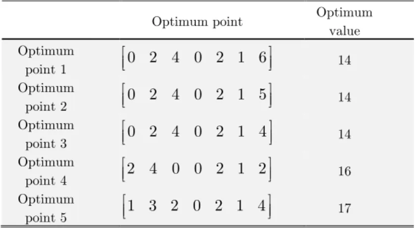
Using the present algorithm, 3 global and 2 local optimal points are obtained after 45 iterations, which take 2.484 sec to converge. Table 4 shows the optimum points and their corresponding optimum values.

Optimum point Optimum

value Optimum

point 1 0 2 4 0 2 1 6

é ù

ê ú

ë û 14

Optimum

point 2 éêë0 2 4 0 2 1 5ùúû 14 Optimum

point 3 éêë0 2 4 0 2 1 4ùúû 14 Optimum

point 4 2 4 0 0 2 1 2

é ù

ê ú

ë û 16

Optimum

point 5 éêë1 3 2 0 2 1 4ùúû 17

(15)

Example 8: This example is taken from (Deep et al., 2009).

1

2 9

2

1 3

( )

min (x) exp 0.01

x i

i

u x

f i

x

=

é æ_ç _- ö_÷ ù

ê ç ÷ ú

= _ê _ç_ç- ÷_÷- _ú

÷

çè ø

ê ú

ë û

å

(

)

2/3

25 50 ln(0.01 ) . :

i

u i

S T

= +

-1

0£x £ 5

{

}

2 0,1, , 25

x Î 

{

}

3 1, 2, ,100

x Î 

The global optimum point is x_opt = ê_ëé1.5 25 50ù_ú_ûTwithf(x_opt)= 0. It is in full agreement with

the results reported in other studies.

Example 9: This example is taken from (Costa and Oliveira, 2001).

3 4 5 6

min ( )f x = 5x +7x +6x +7.5x +5.5x

5 6 1

x +x =

(

0.53

)

1 0.9 1 1

x

z = -e- x

(

0.4 4

)

1 0.8 1 2

x

z = -e- x

1 2 0

x +x - =x

1 2 10

z +z =

3 10 5

x £ x

4 10 6

x £ x

1 20 5

x £ x

2 20 6

x £ x

0 1,..., 4

i

x ³ i =

{ }

0,1 5, 6 i

x Î i =

The global optimum point is x_opt = ê_ëé13.4252 0 3.5162 0 1 0ù_ú_ûTwithf(x_opt)= 99.2396. The

optimum value of the cost function is reported as f(x_opt)= 99.245209in (Fogel et al., 1966). As seen,

the proposed method provides a better value for the cost function in comparison to the one reported by Fogle et al.

Example 10: This is an integer cubic problem which is taken from (Dickman and Gilman, 1989).

1 2 3 1 4 5 2 4 6 6 7 8 2 5 7

max ( )f x = -(x x x +x x x +x x x +x x x +x x x )

1 4 8

(16)

1 4 6

41-(11x +7x +13 )x £0

2 4 6 7

60-(6x +9x x +x )£0

2 5 8

42-(3x +5x +7x )£0

2 7 3 5

53-(6x x +9x +5 )x £0

3 7 5

13-(4x x +x )£0

1 2 4 5 7

2x +4x +7x +3x +x £69

1 8 3 5 3 7

9x x +6x x +4x x £47

2 2 8 3 6

12x +x x +2x x £73

3 4 5 2 6 9 8 31

x + x + x + x £

{

0,1,..., 7

}

1, 3, 4, 6, 8 i

x Î i =

{

0,1,...,15

}

2, 5, 7 i

x Î i =

There are eight design variables and ten inequality constraints. The optimum point is

opt

x = êé_ë5 4 1 1 6 3 2 0_û_úùTwith f(x_opt)= -110, which is in full agreement with (Dickman

and Gilman, 1989).

Example 11: This example is taken from (Costa and Oliveira, 2001) and also given in (Lin et al., 2004). The problem contains three integer variables and seven continuous ones subjected to 18 ine-quality constraints.

1

min

. :

j

M

j j j

j

f N V

S T

b a

= =

å

1 N

i Li

i i

Q T H B

=

£

å

j ij i

V ³S B

j Li ij

N T ³ t

1£N_j £Nu_j

l u

j j j

V £V £V

l u

Li Li Li

T £T £T

l u

i i i

B £B £ B

Where, for the specific problem considered in this paper, M=3, N=2, H=6000, j=250, j=0.6,

Nju=3, Vjl=250 and Vju=2500. The values of the other parameters are given as follows:

max ij

l

Li _u

j

t T

N

(17)

Latin American Journal of Solids and Structures 13 (2016) 224-242 max

u

Li ij

T = t

l i i Li Q B T H =

min( , min( ))

u j u i i i j ij V B Q S =

8 20 8

16 4 4

é ù

ê ú

= ê_ê ú_ú

ë û

t

2 3 4 4 6 3

é ù

ê ú

= ê_ê ú_ú

ë û

S

The obtained global optimum point is x_opt = êé_ë1 1 1 480 720 960 240 120 20 16ù_ú_ûT

withf(x_opt)= 38499.8, which is in full agreement with that which was reported in the other studies.

Example 12: This example addresses the optimal design of multiproduct batch plants which is taken from (Goyal and Ierapetritou, 2004) and also given in (Kocis and Grossmann, 1988). This MINLP problem consists of 100 variables, from which 60 are binary ones. The problem contains 217 con-straints and a nonlinear objective function. The problem data can be found in (Goyal and Ierapetritou, 2004).

1

min exp( )

. :

M

j j j j

j

v

S T

f a n b

=

å

+

ln( ) 1,..., 1,...,

j ij i

v ³ S +b i = N j = M

ln( ) 1,..., 1,...,

j Li ij

n +t ³ t i = N j = M

1

exp( )

N

i Li i

i

Q t b H

=

- £

å

1

ln( ) 1,...,

U j N

j kj

k

n k Y j M

=

å

=

1

1 1,...,

U j N

kj k

Li Li Li

T £t £ T j = ,...,M

( )

(18)

Latin American Journal of Solids and Structures 13 (2016) 224-242 The optimal value of the objective function is 2.68×106, and is in full agreement with the value reported in(Goyal and Ierapetritou, 2004).

5. CONCLUSION AND SUMMARY

In this paper, an algorithm was proposed for the solution of constrained, integer and mixed integer, non-linear optimization problems. In this algorithm a deterministic search over the solution space is performed to find the optimal solution. The performance of the proposed algorithm was tested through several integer and mixed integer (including multi-modal) optimization problems. The obtained re-sults were compared with those reported in the literature demonstrating efficiency and fast conver-gence. One of the most important advantages of this method is the ability to find more than one optimal point with only one run of the computer program. So, this algorithm is suitable for multi-modal optimization problems.

References

Abramson, M. A., (2002). Pattern search algorithms for mixed variable general constrained optimization problems. Dissertation, Houston, Texas.

Audet, C., Dennis, J. E., (2001). Pattern search algorithm for mixed variable programming, SIAM J. Optimiz. 11:53-594.

Back, T., Fogel, D. B., & Michalewicz, Z. (1997). Handbook of evolutionary computation. IOP Publishing Ltd. Box, G. E. P., (1975). Evolutionary operation: A method for increasing industrial productivity, J. Appl. Statist. 6:81-101.

Coelho, L. D. S., (2009). An efficient particle swarm approach for mixed-integer programming in reliability–redundancy optimization applications, Reliab. Eng. Syst. Saf. 94:830–837.

Costa, L., Oliveira, P., (2001). Evolutionary algorithms approach to the solution of mixed integer non-linear program-ming problems, Comput. Chem. Eng. 25:257-266.

Dakin, R. J., (1965). A tree-search algorithm for mixed integer programming problems, Comput. J. 8:250-255. Deep, K., Singh, K. P., Kansal, M. L., Mohan, C., (2009). A real coded genetic algorithm for solving integer and mixed integer optimization problems, Appl. Math. Comput. 212:505-518.

Dickman, B. H., Gilman, M. J., (1989). Technical Note: Monte Carlo Optimization, J. Optim. Theory Appl. 60:149-157.

Duran, M. A., Grossman, I. E., (1986). An outer approximation algorithm for a class of mixed integer nonlinear programs, Math. Prog. 36:306-339.

Fletcher, R., Leyffer, S., (1994). Solving mixed integer programs by outer approximation, Math. Prog. 66:327-349. Fogel, L. J., Owens, A. J., Walsh, M. J., (1966). Artificial Intelligence through simulated evolution, John Wiley and Sons(New York).

Geoffrion, A. M., (1972). Generalized benders decomposition, J. Optim. Theory Appl. 10:237-260.

Gidas, B., (1985). Non-stationary Markov chains and convergence of the annealing algorithm, J. Statist. Phys. 39:73-131.

Glover, F., (1990). Tabu search, ORSA J. Comp. 1:4-32.

(19)

Goyal, V., Ierapetritou, M. G., (2004). Computational studies using a novel simplicial-approximation based algorithm for MINLP optimization, Comput. Chem. Eng. 28:1771-1780.

Holland, J. H., (1962). Outline for a logical theory of adaptive systems, J. ACM 3:297-314.

Kelley, J. E., (1960). The cutting plane method for solving convex programs, J. Soc. Indust. and Appl. Math. 8:703-712

Kesavan, P., Barton, P. I., (2000). Generalized branch-and-cut framework for mixed-integer nonlinear optimization problems, Comput. Chem. Eng. 24:1361-1366.

Kocis, G. R., Grossmann, I. E., (1988). Global Optimization of Nonconvex Mixed-Integer Nonlinear Programming (MINLP) Problems in Process Synthesis, Ind. Eng. Chem. Res. 27:1407-1421.

Leyffer, S., (1998). Integrating SQP and branch-and-bound for mixed integer nonlinear programming, Technical Report NA/182, Dundee University.

Lin, Y. C., Hwang, K. S., Wang, F. S., (2004). A coding scheme of evolutionary algorithms to solve mixed-integer nonlinear programming problems, Comput. Math. Appl. 47:1295-1307.

Marchand, H., Martin, A., Weismantel, R., (2002). Laurence Wolsey, Cutting planes in integer and mixed integer programming, Discrete Appl. Math. 123:397-446.

Ponsich, A., Coello, C. A., (2009). Differential Evolution performances for the solution of mixed-integer constrained process engineering problems, Applied Soft Computing. doi:10.1016/j.asoc.2009.11.030.

Schluter, M., Egea, J. A., Banga, J. R., (2009). Extended ant colony optimization for convex mixed integer non-linear programming, Comput. Oper. Res. 36:2217-2229.

Tian, P., Ma, J., Zhang, D. M., (1998). Nonlinear integer programming by Darwin and Boltzmann mixed strategy, Eur. J. Oper. Res. 105:224-235.

Vanderplaats, G. N. (1999). Numerical optimization techniques for engineering design, Vanderplaats Research & De-velopment. Inc., Colorado Springs, CO.

Wang, L., (2009). Cutting plane algorithms for the inverse mixed integer linear programming problem, Oper. Res. Lett. 37:114-116.

Yan, L. X., Ma, D. X., (2001). Global optimization of nonconvex nonlinear programs using line-up competition algo-rithm, Comput. Chem. Eng. 25:1601-1610.