AIMMS Modeling Guide - Integer Programming Tricks

(1)

This ﬁle contains only one chapter of the book. For a free download of the complete book in pdf format, please visitwww.aimms.comor order your hard-copy atwww.lulu.com/aimms.

(2)

Schipholweg 1 2034 LS Haarlem The Netherlands Tel.: +31 23 5511512 Fax: +31 23 5511517

500 108th Avenue NE Ste. # 1085 Bellevue, WA 98004 USA

Tel.: +1 425 458 4024 Fax: +1 425 458 4025

Ltd.

80 Raﬄes Place UOB Plaza 1, Level 36-01 Singapore 048624 Tel.: +65 9640 4182

Email: info@aimms.com WWW:www.aimms.com

Aimmsis a registered trademark of Paragon Decision Technology B.V.IBM ILOG CPLEXand sc CPLEX is a registered trademark of IBM Corporation. GUROBI_{is a registered trademark of Gurobi Optimization,} Inc. KNITROis a registered trademark of Ziena Optimization, Inc. XPRESS-MPis a registered trademark of FICO Fair Isaac Corporation. Mosek_{is a registered trademark of Mosek ApS.}Windows_andExcel_are registered trademarks of Microsoft Corporation. TEX, LA_{TEX, and}_AMS-LA_{TEX are trademarks of the American}

Mathematical Society.Lucida_{is a registered trademark of Bigelow & Holmes Inc.}Acrobat_{is a registered} trademark of Adobe Systems Inc. Other brands and their products are trademarks of their respective holders.

Information in this document is subject to change without notice and does not represent a commitment on the part of Paragon Decision Technology B.V. The software described in this document is furnished under a license agreement and may only be used and copied in accordance with the terms of the agreement. The documentation may not, in whole or in part, be copied, photocopied, reproduced, translated, or reduced to any electronic medium or machine-readable form without prior consent, in writing, from Paragon Decision Technology B.V.

Paragon Decision Technology B.V. makes no representation or warranty with respect to the adequacy of this documentation or the programs which it describes for any particular purpose or with respect to its adequacy to produce any particular result. In no event shall Paragon Decision Technology B.V., its employees, its contractors or the authors of this documentation be liable for special, direct, indirect or consequential damages, losses, costs, charges, claims, demands, or claims for lost profits, fees or expenses of any nature or kind.

In addition to the foregoing, users should recognize that all complex software systems and their doc-umentation contain errors and omissions. The authors, Paragon Decision Technology B.V. and its em-ployees, and its contractors shall not be responsible under any circumstances for providing information or corrections to errors and omissions discovered at any time in this book or the software it describes, whether or not they are aware of the errors or omissions. The authors, Paragon Decision Technology B.V. and its employees, and its contractors do not recommend the use of the software described in this book for applications in which errors or omissions could threaten life, injury or significant loss.

(3)

Chapter

7 Integer Linear Programming Tricks

This chapter

As in the previous chapter “Linear Programming Tricks”, the emphasis is on abstract mathematical modeling techniques but this time the focus is on inte-gerprogramming tricks. These are not discussed in any particular reference, but are scattered throughout the literature. Several tricks can be found in [Wi90]. Other tricks are referenced directly.

Limitation to linear integer programs

Onlylinearinteger programming models are considered because of the avail-ability of computer codes for this class of problems. It is interesting to note that several practical problems can be transformed into linear integer pro-grams. For example, integer variables can be introduced so that a nonlinear function can be approximated by a “piecewise linear” function. This and other examples are explained in this chapter.

7.1 A variable taking discontinuous values

A jump in the bound

This section considers an example of a simple situation that cannot be formu-lated as a linear programming model. The value of a variable must be either zero or between particular positive bounds (see Figure7.1). In algebraic nota-tion:

x=0 or l≤x≤u

This can be interpreted as two constraints that cannot both hold simultane-ously. In linear programming only simultaneous constraints can be modeled.

0 l u x

Figure 7.1: A discontinuous variable

Applications

(4)

Modeling dis-continuous variables

To model discontinuous variables, it is helpful to introduce the concept of an

indicator variable. An indicator variable is a binary variable (0 or 1) that indi-cates a certain state in a model. In the above example, the indicator variabley

is linked toxin the following way:

y=

⎧ ⎨ ⎩

0 forx=0 1 forl≤x≤u

The following set of constraints is used to create the desired properties:

x≤uy

x≥ly

y binary

It is clear thaty=0 impliesx=0, and thaty=1 impliesl≤x≤u.

7.2 Fixed costs

The model

A ﬁxed cost problem is another application where indicator variables are added so that two mutually exclusive situations can be modeled. An example is provided using a single-variable. Consider the following linear programming model (the sign “≷” denotes either “≤”, “=”, or “≥” constraints).

Minimize: C(x)

Subject to:

aix+ j∈J

aijwj≷bi ∀i∈I

x≥0

wj≥0 ∀j∈J

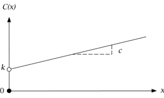
Where: C(x)=

⎧ ⎨ ⎩

0 forx=0

k+cx forx >0

As soon asxhas a positive value, a ﬁxed cost is incurred. This cost function is not linear and is not continuous. There is a jump atx=0, as illustrated in Figure7.2.

Application

(5)

Chapter 7. Integer Linear Programming Tricks 77

C(x)

k

0 x

c

Figure 7.2: Discontinuous cost function

Modeling fixed costs

A suﬃciently large upper bound, u, must be speciﬁed for x. An indicator variable,y, is also introduced in a similar fashion:

y=

⎧ ⎨ ⎩

0 forx=0 1 forx >0

Now the cost function can be speciﬁed in bothxandy:

C∗_{(x, y)}₌_ky₊_cx

The minimum of this function reﬂects the same cost ﬁgures as the original cost function, except for the case when x > 0 and y = 0. Therefore, one constraint must be added to ensure thatx=0 whenevery=0:

x≤uy

The equivalent mixed integer program

Now the model can be stated as a mixed integer programming model. The formulation given earlier in this section can be transformed as follows.

Minimize: ky+cx

Subject to:

aix+ j∈J

aijwj≷bi ∀i∈I

x≤uy x≥0

wj≥0 ∀j∈J

y binary

7.3 Either-or constraints

The model

Consider the following linear programming model:

Minimize:

(6)

Subject to:

j∈J

a1jxj≤b1 (1)

j∈J

a2jxj≤b2 (2)

xj≥0 ∀j∈J

Where: at least one of the conditions (1) or (2) must hold

The condition that at least one of the constraints must hold cannot be for-mulated in a linear programming model, because in a linear programall con-straints must hold. Again, a binary variable can be used to express the prob-lem. An example of such a situation is a manufacturing process, where two modes of operation are possible.

Modeling either-or constraints

Consider a binary variabley, and suﬃciently large upper boundsM1andM2, which are upper bounds on the activity of the constraints. The bounds are chosen such that they are as tight as possible, while still guaranteeing that the left-hand side of constraintiis always smaller thanbi+Mi. The constraints

can be rewritten as follows:

(1) j∈J

a1jxj≤b1+M1y

(2) j∈J

a2jxj≤b2+M2(1−y)

When y = 0, constraint (1) is imposed, and constraint (2) is weakened to

j∈Ja2jxj≤b2+M2, which will always be non-binding. Constraint (2) may of

course still be satisﬁed. Wheny =1, the situation is reversed. So in all cases one of the constraints is imposed, and the other constraint may also hold. The problem then becomes:

The equivalent mixed integer program

Minimize:

j∈J cjxj

Subject to:

j∈J

a1jxj≤b1+M1y

j∈J

a2jxj≤b2+M2(1−y)

xj≥0 ∀j∈J

(7)

7.4 Conditional constraints

The model

A problem that can be treated in a similar way to either-or constraints is one that contains conditional constraints. The mathematical presentation is lim-ited to a case, involving two constraints, on which the following condition is imposed.

If (1) ( j∈J

a1jxj≤b1) is satisfied,

then (2) ( j∈J

a2jxj≤b2) must also be satisfied.

Logical equivalence

LetAdenote the statement that the logical expression “Constraint (1) holds” is true, and similarly, let Bdenote the statement that the logical expression “Constraint (2) holds” is true. The notation ¬A and ¬B represent the case of the corresponding logical expressions being false. The above conditional constraint can be restated as:A implies B. This is logically equivalent to writing

(A and¬B) is false. Using the negation of this expression, it follows that¬(A and¬B)is true. This is equivalent to(¬A or B) is true, using Boolean algebra. It is this last equivalence that allows one to translate the above conditional constraint into an either-or constraint.

Modeling conditional constraints

One can observe that

If ( j∈J

a1jxj≤b1) holds, then ( j∈J

a2jxj≤b2) must hold,

is equivalent to

( j∈J

a1jxj> b1) or ( j∈J

a2jxj≤b2) must hold.

Notice that the sign in (1) is reversed. A diﬃculty to overcome is that the strict inequality “not (1)” needs to be modeled as an inequality. This can be achieved by specifying a small tolerance value beyond which the constraint is regarded as broken, and rewriting the constraint to:

j∈J

a1jxj≥b1+ǫ

This results in:

j∈J

a1jxj≥b1+ǫ, or j∈J

a2jxj≤b2 must hold.

(8)

variabley, a suﬃciently large upper boundM on (2), and a suﬃciently lower boundLon (1). The constraints can be rewritten to get:

j∈J

a1jxj≥b1+ǫ−Ly

j∈J

a2jxj≤b2+M(1−y)

You can verify that these constraints satisfy the original conditional expression correctly, by applying reasoning similar to that in Section7.3.

7.5 Special Ordered Sets

This section

There are particular types of restrictions in integer programming formulations that are quite common, and that can be treated in an eﬃcient manner by solvers. Two of them are treated in this section, and are referred to as Spe-cial Ordered Sets(SOS) of type 1 and 2. These concepts are due to Beale and Tomlin ([Be69]).

SOS1 constraints

A common restriction is that out of a set of yes-no decisions, at most one decision variable can be yes. You can model this as follows. Let yi denote

zero-one variables, then

i

yi≤1

forms an example of a SOS1 constraint. More generally, when considering variables 0≤xi≤ui, then the constraint

i

aixi≤b

can also become a SOS1 constraint by adding the requirement that at most one of thexi can be nonzero. InAimmsthere is a constraint attribute named Propertyin which you can indicate whether this constraint is a SOS1 constraint. Note that in the general case, the variables are no longer restricted to be zero-one variables.

SOS1 and performance

(9)

SOS1 branching

To illustrate how the SOS order information is used to create new nodes during the branch and bound process, consider a model in which a decision has to be made about the size of a warehouse. The size of the warehouse should be either 10000, 20000, 40000, or 50000 square feet. To model this, four binary variables x1, x2, x3 and x4 are introduced that together make up a SOS1 set. The order among these variables is naturally speciﬁed through the sizes. During the branch and bound process, the split point in the SOS1 set is determined by the weighted average of the solution of the relaxed problem. For example, if the solution of the relaxed problem is given byx1 =0.1 and

x4=0.9, then the corresponding weighted average is 0.1·10000+0.9·50000= 46000. This computation results in the SOS set being split up between variable

x3 andx4. The corresponding new nodes in the search tree are speciﬁed by (1) the nonzero element is the set{x1, x2, x3}(i.e.x4=0) and (2)x4=1 (and

x1=x2=x3=0).

SOS2 constraints

Another common restriction, is that out of a set of nonnegative variables, at most two variables can be nonzero. In addition, the two variables must be adjacent to each other in a ﬁxed order list. This class of constraint is referred to as a type SOS2 inAimms_{. A typical application occurs when a non-linear} function is approximated by a piecewise linear function. Such an example is given in the next section.

7.6 Piecewise linear formulations

The model

Consider the following model with a separable objective function:

Minimize:

j∈J fj(xj)

Subject to:

j∈J

aijxj≷bi ∀i∈I

xj≥0 ∀j∈J

Separable function

In the above general model statement, the objective is a separable function, which is deﬁned as the sum of functions of scalar variables. Such a func-tion has the advantage that nonlinear terms can be approximated by piecewise linear ones. Using this technique, it may be possible to generate an integer pro-gramming model, or sometimes even a linear propro-gramming model (see [Wi90]). This possibility also exists when a constraint is separable.

Examples of separable functions

Some examples of separable functions are:

x2

(10)

The following examples are not:

x1x2+3x2+x2₂=f1(x1, x2)+f2(x2)

1/(x1+x2)+x3=g1(x1, x2)+g2(x3)

Approximation of a nonlinear function

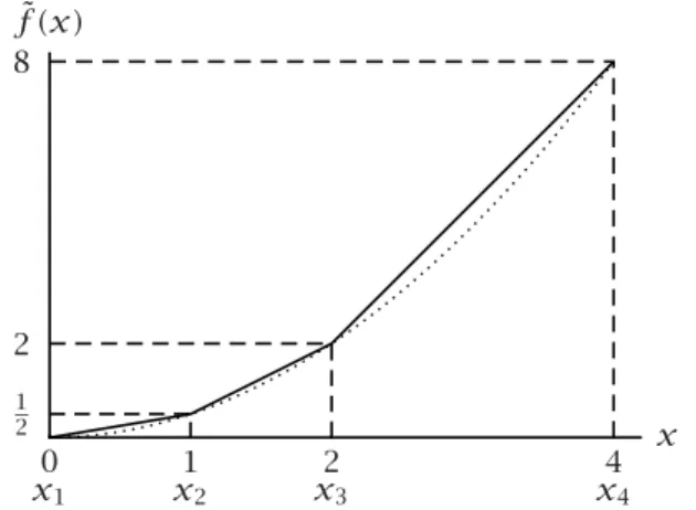
Consider a simple example with only one nonlinear term to be approximated, namelyf (x)=1₂x2_{. Figure}_7.3_{, shows the curve divided into three pieces that}

are approximated by straight lines. This approximation is known as piecewise linear. The points where the slope of the piecewise linear function changes (or its domain ends) are referred to as breakpoints. This approximation can be ex-pressed mathematically in several ways. A method known as theλ-formulation is described below.

x

˜

f (x)

0

x1 x21 x32 x44

1 2

2 8

Figure 7.3: Piecewise linear approximation off (x)=1₂x2

Weighted sums

Letx1, x2, x3andx4denote the four breakpoints along the x-axis in Figure7.3, and letf (x1), f (x2), f (x3)andf (x4)denote the corresponding function val-ues. The breakpoints are 0, 1, 2 and 4, and the corresponding function values are 0, 1₂, 2 and 8. Any point in between two breakpoints is a weighted sum of these two breakpoints. For instance,x=3= 1₂·2+1₂·4. The corresponding approximated function value ˜f (3)=5=1₂·2+1₂·8.

λ-Formulation

Let λ1, λ2, λ3, λ4 denote four nonnegative weights such that their sum is 1. Then the piecewise linear approximation off (x)in Figure7.3can be written as:

λ1f (x1)+λ2f (x2)+λ3f (x3)+λ4f (x4)=f (x)˜ λ1x1+λ2x2+λ3x3+λ4x4=x

λ1+λ2+λ3+λ4=1

(11)

con-Chapter 7. Integer Linear Programming Tricks 83

straint referred to at the end of the previous section. The SOS2 constraints for all separable functions in the objective function together guarantee that the points(x,f (x))˜ always lie on the approximating line segments.

Adjacency requirements sometimes redundant

The added requirement that at most two adjacent λ’s are greater than zero can be modeled using additional binary variables. This places any model with SOS2 constraints in the realm of integer (binary) programming. For this reason, it is worthwhile to investigate when the added adjacency requirements are redundant. Redundancy is implied by the following conditions.

1. The objective is to minimize a separable function in which all terms

fj(xj)areconvexfunctions.

2. The objective is to maximize a separable function in which all terms

fj(xj)areconcavefunctions.

Convexity and concavity

A function is convex when the successive slopes of the piecewise linear approx-imation are nondecreasing, and concave if these slopes are non-increasing. A concave cost curve can represent an activity with economies of scale. The unit costs decrease as the number of units increases. An example is where quantity discounts are obtained.

The case of a non-convex function

The adjacency requirements are no longer redundant when the function to be approximated is non-convex. In this case, these adjacency requirements must be formulated explicitly in mathematical terms.

SOS2 inAimms InAimms_{you do not need to formulate the adjacency requirements explicitly.}

Instead you need to specifysos2 in thepropertyattribute of the constraint in which the λ’s are summed to 1. In this case, the solver inAimms guarantees that there will be at most two adjacent nonzero λ’s in the optimal solution. If the underlying minimization model is convex, then the linear programming solution will satisfy the adjacency requirements. If the model is not convex, the solver will continue with a mixed integer programming run.

7.7 Elimination of products of variables

This section

(12)

Replacing product term

In general, a product of two variables can be replaced by one new variable, on which a number of constraints is imposed. The extension to products of more than two variables is straightforward. Three cases are distinguished. In the third case, a separable function results (instead of a linear one) that can then be approximated by using the methods described in the previous section.

Two binary variables

Firstly, consider the binary variablesx1 and x2. Their product,x1x2, can be replaced by an additional binary variabley. The following constraints force y to take the value ofx1x2:

y≤x1

y≤x2

y≥x1+x2−1

y binary

One binary and one continuous variable

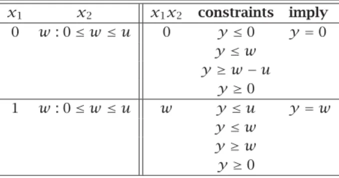
Secondly, letx1be a binary variable, andx2be a continuous variable for which 0≤x2 ≤uholds. Now a continuous variable,y, is introduced to replace the producty=x1x2. The following constraints must be added to forcey to take the value ofx1x2:

y≤ux1

y≤x2

y≥x2−u(1−x1) y≥0

The validity of these constraints can be checked by examining Table 7.1 in which all possible situations are listed.

x1 x2 x1x2 constraints imply

0 w: 0≤w≤u 0 y≤0 y=0

y≤w y ≥w−u

y≥0

1 w: 0≤w≤u w y≤u y=w

y≤w y≥w y≥0

(13)

Two continuous variables

Thirdly, the product of two continuous variables can be converted into a sep-arable form. Suppose the productx1x2must be transformed. First, two

(con-tinuous) variablesy1andy2are introduced. These are deﬁned as:

y1=1

2(x1+x2)

y2=1

2(x1−x2)

Now the termx1x2can be replaced by the separable function

y2 1−y22

which can be approximated by using the technique of the preceding section. Note that in this case the non-linear term can be eliminated at the cost of having to approximate the objective. If l1≤x1≤u1andl2≤x2≤u2, then the bounds ony1andy2are:

1

2(l1+l2)≤y1≤ 1

2(u1+u2) and 1

2(l1−u2)≤y2≤ 1

2(u1−l2)

Special case

The productx1x2can be replaced by a single variablezwhenever

the lower boundsl1andl2are nonnegative, and

one of the variables is not referenced in any other term except in prod-ucts of the above form.

Assume, that x1 is such a variable. Then substituting for z and adding the constraint

l1x2≤z≤u1x2

is all that is required to eliminate the nonlinear termx1x2. Once the model is solved in terms ofz andx2, thenx1 =z/x2 whenx2 >0 anx1 is undeter-mined whenx2 =0. The extra constraints onz guarantee thatl1 ≤x1≤u1

wheneverx2>0.

7.8 Summary

(14)

[Be69] E.M.L. Beale and J.A. Tomlin,Special facilities in a general mathemati-cal programming system for non-convex problems using ordered sets of variables, Proceedings of the 5th International Conference on Opera-tions Research (Tavistock, London) (J. Lawrence, ed.), 1969.