Learning oncogenetic networks by reducing to mixed integer linear programming.

Integer Linear Programming

Hossein Shahrabi Farahani, Jens Lagergren*

KTH Royal Institute of Technology, Science for Life Laboratory (SciLifeLab), Center for Industrial and Applied Mathematics, School of Computer Science and Communication, Stockholm, Sweden

Abstract

Cancer can be a result of accumulation of different types of genetic mutations such as copy number aberrations. The data from tumors are cross-sectional and do not contain the temporal order of the genetic events. Finding the order in which the genetic events have occurred and progression pathways are of vital importance in understanding the disease. In order to model cancer progression, we proposeProgression Networks, a special case of Bayesian networks, that are tailored to model disease progression. Progression networks have similarities with Conjunctive Bayesian Networks (CBNs) [1],a variation of Bayesian networks also proposed for modeling disease progression. We also describe a learning algorithm for learning Bayesian networks in general and progression networks in particular. We reduce the hard problem of learning the Bayesian and progression networks to Mixed Integer Linear Programming (MILP). MILP is a Non-deterministic Polynomial-time complete (NP-complete) problem for which very good heuristics exists. We tested our algorithm on synthetic and real cytogenetic data from renal cell carcinoma. We also compared our learned progression networks with the networks proposed in earlier publications. The software is available on the website https://bitbucket.org/farahani/diprog.

Citation:Shahrabi Farahani H, Lagergren J (2013) Learning Oncogenetic Networks by Reducing to Mixed Integer Linear Programming. PLoS ONE 8(6): e65773. doi:10.1371/journal.pone.0065773

Editor:Jian-Xin Gao, Shanghai Jiao Tong University School of Medicine, China

ReceivedDecember 7, 2012;AcceptedApril 28, 2013;PublishedJune 14, 2013

Copyright:ß2013 Shahrabi Farahani, Lagergren. This is an open-access article distributed under the terms of the Creative Commons Attribution License, which permits unrestricted use, distribution, and reproduction in any medium, provided the original author and source are credited.

Funding:Funding provided by the Center for Industrial and Applied Mathematics, website: http://www.ciam.kth.se/en. The funders had no role in study design, data collection and analysis, decision to publish, or preparation of the manuscript.

Competing Interests:The authors have declared that no competing interests exist.

* E-mail: jensl@csc.kth.se

Introduction

Mutations of single nucleotides but also structural changes, e.g., deletions, duplications, inversions, and translocations of genomic segments, as well as epigentic modifications have all been implicated in cancer. Traditionally cytogenetic techniques have been used to characterize structural aberrations in tumors and more recently Comparative Genomic Hybridization (CGH) arrays have been used to reveal Copy Number Aberrations (CNA). Today, genomics resequencing, exon resequencing, and RNA-Seq are the methods of choice for assaying cancer tumors. Although this constitutes a remarkable technological development and today’s data are in many aspects unprecedented, cancer data is and will continue to be mainly cross-sectional. That is, for each of a number of patients, a single tumor is removed at one time point and assayed, which gives information about the set of aberrations in the tumor. However, aberrations occur sequentially in time and, also, one aberration can yield another aberration, by making the second favorable for the tumor (a good example is that an aberration causing angiogenesis is favorable to a tumor subse-quent, but not previous, to an aberration causing increased tumor size). In fact, it is of central importance that cancer progresses and is a historical process in which the next event depends on those already having occurred. Mathematical models of cancer progression and corresponding learning algorithms are required in order to facilitate inference of cancer progression pathways, i.e., the set of favorability relations between aberrations.

Vogelstein et al. [2] suggested a path-based model of colorectal cancer progression consisting of 4 genetic events. This is a

biomedical model that can be viewed as a starting point for a development of a series of mathematical models. Due to the complexity of cancer, it is desirable to base cancer models on more complex discrete structures than paths. Tree-based models are clearly more general than paths, but they do unfortunately not allow different progression paths to converge. Consequently, a substantial modeling effort has led the area to evolve from considering path-based models to tree-based models and beyond. Desper et al. [3] suggested tree based models that are non-probabilistic, i.e., how well an individual model describe a data set cannot be assigned a probability. Beerenwinkel et al. [4] used probabilistic tree-based models and mixtures of such models. They also gave ‘‘EM-like’’ algorithms for learning these models. The original application was analysis of HIV data but later also cancer data was analyzed [5]. these results were subsequently improved by introduction of Hidden Variable Oncogenetic Trees (HOTs) that have a monotonicity property well-adapted to model disease progression as well as latent variables which yields a better capacity to describe noise by experimental data [6]. Global structural EM-algorithms for learning these models were also described [6].

network model with a monotonicity property. Conjunctive Bayesian networks are similar to noisy-AND models in the AI literature [9]. CBNs are not well-suited to learn noisy experimental data. Gerstung at al. [10] address this problem by proposing Hidden CBN (H-CBN) where the variables of a CBN are considered latent and visible variables have a 1-to-1 correspon-dence to these latent variables.

In a pioneering line of work Ho¨glund et al. [11–13] used a non-probabilistic method, which incorporates Principal Component Analysis (PCA) on the pairwise correlation between aberrations and to a large extent depends on human decision and, therefore, is somewhat orthogonal to the methods described above. Cussens [14] used integer programming in pedigree reconstruction problem. Pedigrees can be seen as Bayesian networks.

Recently, by introduction of high-throughput sequencing technologies, sequencing of small collection of tumor genomes have become feasible. The temporal order of somatic mutations (point mutations and structural rearrangements) that have created a tumor genome from a germ line genome are not immediately revealed from these genomes. Greenman et al. [15] proposed an algorithm for reconstructing the events sequence of a single tumor. In a recent effort Nik-Zainal et al. [16] applied the Greenman algorithm [15] to 21 breast cancer tumors.

Gerstung and colleagues [17] observed that tumors from the same type of cancer often show a few genetic alterations in common. They hypothesized that temporal order of the events in a tumor may act on the pathway level rather than the gene level. According to their hypothesis, mutations in the genes that are involved in the same functional pathway can partly explain the heterogeneity in the tumors. After mapping the genes to the functional pathways, they applied the H-CBN algorithm on the pathway level. Cheng et al. [18] used the same approach to determine whether specific pathway alterations appear early or late during the tumor progression.

Methods

Notation

Learning cancer progression networks give rise to hard computational problems. In order to obtain biologically sound solutions, we need a lot of notations and mathematical apparatus. The notations and mathematical tools that are used in the paper are introduced in this section.

We use hypergraphs to represent the dependence structures of Bayesian networks. In this section, we introduce key concepts and notation for hypergraphs. We will use ½n to denote the set f1,. . .,ng. AhypergraphH consists of avertex set, denotedV(H), and a set of non-empty subsets ofV(H)calledhyper-edges, denoted E(H). In a graph with standard meaning, all edges are 2-element subsets ofV(H). In other words, in a standard graph each edge connects two vertices. We will consider directed hypergraphs where each hyper-edgeehas a unique child, denotedc(e), and a set of

parents, denotedPa(e). An alternative terminology would be to call c(e)the head ofeandPa(e)its tail. However, using the terms child and parents fits the terminology of our application better. A directed hypergraph H is acyclic if there is a linear order , on V(H) such that for every hyper-edge e[_E(H) and p[_Pa(e), pvc(e)_{. A hyperDAG is a directed acyclic hypergraph. A k-uniform}

hypergraph (k-bounded) is a hypergraph in which all hyper-edges contain exactly (at most)k-vertices. This means that a graph (with the standard meaning) is a 2-uniform hypergraph.

The Models

We here describe the standard Bayesian network model and our models aimed to capture disease progression.

Bayesian and progression networks. We first introduce additional notation. We will typically consider a set of r.v.s X1,. . .,Xn. Assume I5½n. We will use X(I) to denote the set fXi:i[Ig. We will usex(I)to denote assignments toX(I), i.e., an assignmentX(I):?_f0,1g. In particular,x(I)~1denotes that all variables inX(I) are assigned the value 1 and x(I)~0denotes that all variables inX(I)are assigned the value 0.

A Bayesian Network (BN) is pair(H,H), where H~(V,E) is a hyperDAG and H maps edges of H to Conditional Probability Distributions (CPDs), such that: (1) for eachv[_{V(H), there is an}

associated r.v.Xvand (2) for each hyper-edgee[E(H),H(e)is the CPDPr½X(c(e))DX(Pa(e)). Also, we will say that a BN(H,H)is k-boundedif the hypergraphHisk-bounded.

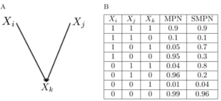
We now introduce our model of disease progression. A BN is called monotone if all its r.v.s are monotone, i.e., for some small constant e and for each hyper-edge e, Pr½X(c(e))~1DX(Pa(e))=1ve. The interpretation of this model is that in order to make the child aberration advantageous to the tumor all parental aberration must have occurred. A r.v. in a BN is calledsemi-monotoneif it only has non-negligible probability to be 1 in case at least one parent is 1. Formally a BN is called semi-monotone if all its r.v.s are semi-monotone, i.e., for some small constant e and for each hyper-edge e, Pr½X(c(e))~1DX(Pa(e))~0ve. The interpretation of this model is that in order to make the child aberration advantageous to the tumor at least on parental aberration must have occurred. Monotone and semi-monotone BNs are collectively refereed to asProgression Networks(PNs).

Figure 1(A) shows a hyper–edge with three r.v.sXi,Xj, andXk. The columns that are labeled MPN and SMPN in Figure 1(B) are monotone and semi-monotone CPDs for the hyper–edge in Figure 1(A), respectively. Conjunctive Bayesian Networks that are proposed by Beerenwinkel and collaborators is a special case of our monotone BNs withe~0, see [1].

Learning ak-bounded Bayesian Network

In this section, we will show how learning ak-bounded BN can be reduced to the problem Maximum Weight k-Bounded Subhypergraph (MWkBS) for a weightedk-bounded hypergraph called the selector graph and, then, how this problem can be reduced to a Mixed Integer Linear Program (MILP). Solving a MILP problem is one, out of several NP-complete problems, for which very good heuristics have been designed. We apply the popular approach of reducing another problem to a MILP rather

Figure 1. The figure shows a hyper–edge and its correspondig CPDs.A sample hyper–edge with 3 r.v.s (a) and monotone and semi– monotone CPDs forPr½XkDXi,Xjthat hyper-edge (b).

than developing new heuristics. We do so since by reducing the problem of learning a Bayesian network with bounded number of parents, for each random variable, to a MILP, we obtain a fast heuristic for the former problem. The algorithm can work with any decomposable score such as maximum likelihood score or Bayesian Information Criterion (BIC) score.

The reduction to MWkBS assigns weights in a fairly standard way, i.e., using Maximum Likelihood (ML) estimated parameters, so that the weight used is exactly what the edge contributes to the overall score of the Bayesian network. We first define weights corresponding to the ML score and, then, we show how to modify them in order to obtain weights corresponding to the BIC score. We could equivalently, as is common, use the mutual information betweenc(e)andPa(e)as the weight of the hyperedgee, see [19]. Also, since we consider decomposable scores, the weight of an edge is the same in any Bayesian network with parameters optimal for the score, which we show explicitly for the BIC score.

Assume thatfX1,. . .,Xngis a set of r.v.s andQis a subset of it. Let D be a dataset and #D the size of the dataset. For any assignmenta:Q?f0,1g, let#_DadenoteDfx[D:xD_Q~agDwhere xDQdenotes the functionxrestricted to the domainQ. Define thek -bounded selector hypergraphSforDas follows. The vertex set is V~½nzk, where ½nare indices corresponding to our r.v.s and fnz1,. . .,nzkgis a special set of vertices calledroot parents, which we denoteR. The root parents are used for technical reasons as parents of vertices that otherwise would not have parents in the subDAG that finally is selected. Let S be obtained from the completek-bounded hypergraph on½nzk(i.e., having all possible edges) by removing all edges with a child inR. The weight of an hyperedge will be defined below so that it depends only on its parents that are not root parents.

LetB~(H,H)be a BN. The log-likelihood ofB, log Pr½DDB, equals.

X

x[D

log Pr½xDB~X

x[D X

e[E(H)

log Pr½x(c(e))Dx(Pa(e)),H(e)~

X

e[E(H) X

x(e)

#Dx(e) log Pr½x(c(e))Dx(Pa(e)),H(e)

GivenH, we definePa0(e)as the set of the parents ofethat are not root parents. IfPa0(e)is not the empty set, the ML estimate of Hare given by

Pr½x(c(e))Dx(Pa(e)),H(e)~ #Dx(e)

#Dx(e)_DPa0 (e)

: ð1Þ

In a BN that is not monotone or semi-monotone for each edge ofH, we define a weightw(e)by

w(e)~X

x(e)

#Dx(e) log

#Dx(e) #Dx(e)

DPa0(e)

: ð2Þ

If the parent vertices in a hyper–edge e consist only of root parents, the weight of e depends only on the child vertex c(e). Then weight of the hyper–edgeecan be calculated according to Equation 3

w(e)~X

x(e)

#Dx(e) log #Dx(e)

#D :

ð3Þ

If some parents in a hyperedgee are root parents, instead of w(e) we use weight of another hyperedge e’ in which Pa(e’)~Pa(e){Randc(e)~c(e’). In other words when calculat-ing the weight of a hyperedge in which some of the parents are the root parents, we ignore the root parents.

In the MPNs there is an upper bound e on Pr½X(c(e))~1DX(Pa(e))=1. As explained before, this upper bound is applied to impose the monotonicity in the learned PN by penalizing the weight of the hyper’ edges in which the child vertex is 1 while not all parent vertices are 1. For learning MPNs we calculate all the probabilities according to Equation 1 except for the cases that Pr½X(c(e))~1DX(Pa(e))=1we in which the weight is set to e. For learning SMPNs the upper bound e is applied toPr½X(c(e))~1DX(Pa(e))~0.

In short, for each hyperedge a CPD like the CPD in Figure 1(B) is calculated using equation 1. In case of MPNs and SMPNs, according to their definitions, the upper bound, e, must be enforced. The values of numerator and denominator of equation 1 can be calculated from the statistics of different CNAs in the dataset according to the definition of#Dain the beginning of this section. Using the computed CPDs, then the weight of each hyperedge is calculated by equations 2 or 3.

Notice that log Pr½DDB~ P

e[E(H)

w(e). Also notice, the weight

of the hyperedgeeis independent of the rest ofH, i.e., it is the same for anyk-bounded hyperDAG containinge. We define the weight of e in S to be the weight it assumes in each of these DAGs. From this follows that, H is a maximum weight k -bounded subhyperDAG ofS if and only ifHtogether with ML estimated parameters induce a BN that maximizes the likelihood of the data.

Again, the weights that are defined above correspond to the log-likelihood or equivalently log-likelihood score, see [19]. When learning from noisy data using the log-likelihood score the resulting BN is typically fully connected [19]. To avoid this type of behavior Schwarz et al. [20] proposed the Bayesian Information Criterion (BIC). In contrary to the likelihood score, the BIC score provides an inclination to use simpler structures. With increasing size of the data set, however, it tends to allow more complex structures to be learned. The BIC weight of an hyperedgee,wBIC(e), is,

wBIC(e)~w(e){ logM

2 Dim(e)

whereMis the size of the dataset andDim(e) is the number of independent parameters in the hyperedgee.

We now describe a MILP, denotedMILP(S), for identifying a maximum weightk-bounded subhyperDAG of a selector graphS

and, thereby, complete the description of our algorithm for learning BNs. The variables of MILP(S) are: (1) hyperedge variablesV_e[_E(S), the variablehe[f0,1gand: (2) order variables

V_i[_V(S), the variableoi[½0,1.

The objective function ofMILP(S)is:

P e[E(S)

hewBIC(e),

wherewBIC(e)is the BIC score ofein the selector graphS. The conditions of MILP(S) are: (1) non-root parents have exactly one incoming edge, i.e.,

V_v[_V(S)\R, X e[E(S):c(e)~v

he~1

and (2) acyclic ordering of the vertices (child higher than parent), i.e.,

V_e[_E(S),p[_Pa(e),he{1vo_c(e){op:

Maximizing the objective function with conditions (1) and (2) results in learning the BN with the highest score. The second condition inMILP(S)guarantees that the hypergraph induced by the program is acyclic. Because hyperedges can not contain a cycle, in each hyperedge the order variable of each parent vertex is smaller than the order variable of the child vertex. Otherwise, for at least one of the parentsoc(e){opv0_{and consequently}h_ev1_.

Becausehe is a binary variable,he~0. We can, hence, conclude the solution of MILP(S) will not contain a cycle.

Results

This section contains the results of our experiments with synthetic data as well as real cytogenetic data. The synthetic data was sampled from 2 and 3-bounded BNs of all three types (i.e.,

MPN, SMPN, and general BNs). We learned each data set with all three variations of our algorithm.

Our main focus was the relation between aberrations. So, in order to measure the performance of our algorithm, we considered the underlying directed simple graphs of hyperDAGs in which for each parent and child of a hyper edge there is a directed edge from the parent to the child. To compare edge sets, we used the percentage of the recovered directed edges, as well as therelative symmetric difference, which takes both sensitivity and specificity into account. Let Mand L be the set of edges in the true and the learned underlying graph, respectively. The relative symmetric difference,F, is defined as follows:

F~DM\LDzDL\MD

DLDzDMD ð4Þ

Furthermore, the values of false discovery rateFDR~DL\MD DLD and false negative rate FNR~DM\LD

DMD are provided separately in the supplementary material.

Synthetic Data

We sampled data from random PNs and then tested the ability of our algorithms to learn the true models. In order to test our algorithms, we generated BNs using all possible combinations of

N

N

N

Synthetic data sets were created by sampling 500, 2000, and 10000 times from each such BN. In both monotone and semi-monotone PNse~0:2. We chose the sample size 500 to show the

performance of DiProg on the existing datasets, which are relatively small. The sizes of tumor datasets are constantly increasing. To measure performance of DiProg on the future larger datasets, we also tested DiProg performance on datasets with 2000 and 10000 samples.

We generated 50 DAGs from each combination. The percent-ages of recovered edges in Figures 2(A)–2(F) are averpercent-ages over 50 DAGs. Tables S1 and S2 show the percentage of the recovered edges and the relative symmetric difference when the network is learned with each of the three variations of the algorithm. Each variation of the DiProg algorithm performs best when the data is generated with the same variation. Tables S3 and S4 include the percentages of false positives and false negatives for each variation of DiProg.

All experiments were performed on a system with two quad-core Intel Harpertown 2.66 GHz CPUs (E5430) and 8 Gb of RAM, with a 64-bit Linux kernel installed. In our tests, we assigned 6 Gb of memory and a limited amount of time proportional to the number of variables and the value ofk. The default value for maximum CPU time for each problem instance is accessible in DiProg’s help. When CPLEX did not find a provably optimal solution in the assigned time or memory constraints, we picked the best incumbent solution available in the solution pool. For each problem, DiProg receives maximum allocated time and memory as arguments.

Figure 2. Percentage of recovered edges when data is generated with monotone, semi-monotone, and general networks and learned with the same method for 2 and 3-bounded graphs.The error bars show 1 standard deviation.

doi:10.1371/journal.pone.0065773.g002

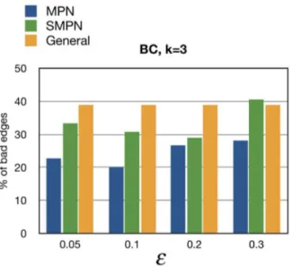
Figure 3. The percentage of bad edges for various values ofe andk~3for MPN, SMPN, and General PNs for BC learned by DiProg.

Cancer Data

We tested the DiProg algorithm on renal cell carcinoma (RCC) using the data from [21]. We also compared the results from DiProg algorithm with the H-CBN algorithm from [10].

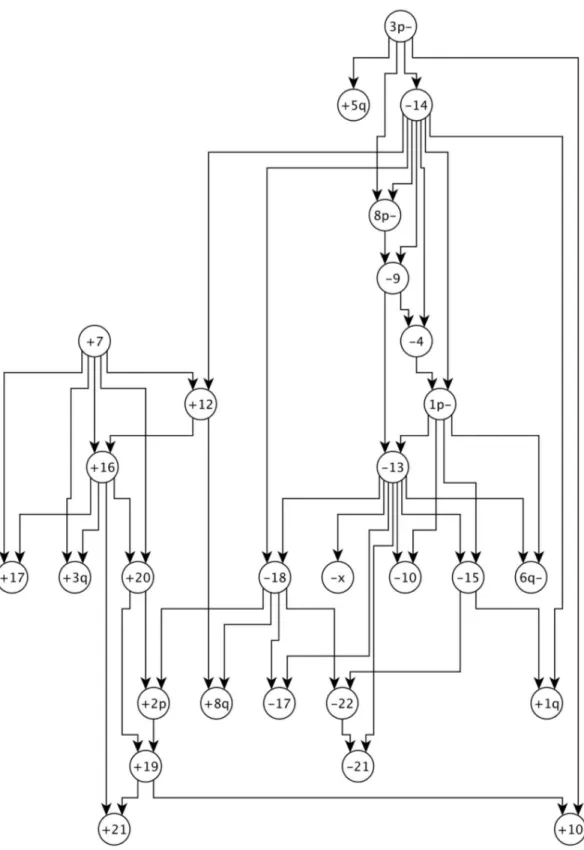
Comparing the results with non-probabilistic methods. In [11] a dataset of 796 RCC tumors with 28 chromosomal aberrations is used. The data was retrieved from Mitelman Database of Chromosome Aberrations in Cancer [21]. Figure 4. The learned MPN for RCC data withk~3ande~0:2.+sign stands for gain and2sign stands for loss in a chromosome arm. Long

To facilitate comparing our results with those in [11], we used the same dataset.

The MPN and SMPN models have a free parameter, i.e.,e. We took advantage of the breast cancer (BC) data from [13] to find a biologically realistic value ofeby identifying the value that gave the best correspondence between the progression network that we obtained and the network proposed for BC in [13]. This was in practice accomplished by choosing the value ofe that gave the minimum fraction of bad edges relative to the number of learned edges. Following [6], we define a bad edge to be an edge in our learned PN that contradicts the partial order imposed by the progression pathways in [13]. In calculating the percentage of bad edges the edges incidents to the root parents are also counted. Figure 3 shows the percentage of bad edges in the breast cancer data from [13] withk~3for various values ofe. A very interesting observation is that for each value ofethe percentage of bad edges in the learned MPNs is less than the semi-monotone and general learned PNs. Figures S1 and S2 show the percentage of bad edges in the learned BC PNs withk~2andk~4for various values ofe. As illustrated in Figure S2, the percentage of bad edges in the learned MPN is also less than those of the learned SMPN and General, except fore~0:3. In the latter case, the large value ofe

effectively weakens the monotonicity condition.

Table S5 shows the percentage of bad edges and BIC scores of the learned MPNs with different values of k and e. For the percentage of bad edges in the learned SMPNs and general BNs see Tables S6 and S7. For a discussion about choosing the value of esee Text S1.

Table S8 contains the BIC scores for MPNs that are learned from RCC data in [11]. For the chosen value ofe~0_:2, the MPN

with k = 3 has the best BIC score. Figure 4 is the MPN that is learned by DiProg algorithm withk~3ande~0:2from the RCC

data in [11]. The progression network for RCC that is proposed in [11] consists of two pathways, one progression pathway starts with loss3p{ and another one starts with gains z7 and z10 and continues withz17,z16, and their descendants. In our learned MPN these two pathways are distinctly separated. Most of the aberrations in the pathway in Figure 5 of [11] that starts with gains

z7andz10are captured in the sub-graph of our learned MPN that consists of the descendants of gain z7. Most of the aberrations in the second pathway in [11] are captured by the component in our MPN that starts with the loss 3p{ and continues with{14and its descendants.

Comparison with the H-CBN algorithm. We compared the results of the DiProg with the H-CBN algorithm. Gerstung et al. [10] used RCC specific CGH data from Progenetics database [22]. Due to limitations in the number of variables that the H-CBN algorithm can handle, they restricted their analysis to 12 variables and 251 tumors in the RCC. In the previous section we presented the results of DiProg on a larger dataset from RCC with 28 variables. In order to be able to compare results of DiProg with H-CBN, in this section we applied DiProg to the smaller dataset with 12 variables. Text S2 contains a discussion about choosing the best value fork. Figure 5 illustrates the MPN that is learned by DiProg withk~3ande~0:2. The learned MPNs by

DiProg are similar to the networks that are proposed in [10] and [23]. It is noteworthy to mention that the authors in [10] rejected the network that was originally learned by the H-CBN algorithm because it only contains two edges. In order to learn a better network, they used the network proposed by Jiang et al. [23] as the starting point for a structure search by the H-CBN algorithm. So, the proposed network for RCC in [10] is sub-optimal according to the H-CBN algorithm. The network learned by DiProg is more similar to the network in [23] than the network in [10]. This shows the reliability of the DiProg results.

Discussion

We propose new algorithms based on mixed integer linear programming (MILP) for learning BNs. Because we are especially interested in modeling disease progression, we used monotone and semi-monotone progression networks. Results from the synthetic data show that depending on the upper bound on the number of parents in monotone and semi–monotone PNs, we can learn the majority of the edges in the generating model.

Because cancer progression is a historical process, it is reasonable to assume that later aberrations need earlier aberra-tions to have occurred before they can be introduced to the cell. To force this monotonicity in learning the progression networks, we defined MPNs and SMPNs. In MPNs, in each hyperedge there is an upper bound on the probability of the child vertex being in the tumor if not all its parents have happened. This makes MPNs more suitable for modeling cancer progression comparing to the general BNs with no such upper bounds.

We also applied our algorithm to cytogenetic data from [11]. In contrast to the semi-automatic method by Ho¨glund et al., DiProg is automatic and,therefore, needs less support by human decision. Furthermore DiProg is based on probabilistic models, which can generate synthetic data and assign a likelihood to the biological data. Also comparing our algorithm with the H-CBN algorithm [10] on the same smaller dataset from RCC shows that DiProg results are in agreement with the previously published results. Comparing to the H-CBN algorithm, DiProg can handle substantially more variables. To illustrate this we presented the Figure 5. The learned MPN for RCC data withk~3ande~0_:2.

The smaller dataset in [10] is used.+sign stands for gain and2sign stands for loss in a chromosome arm. Long and short arms of each chromosome are denoted byqandp, respectively.

results of DiProg on synthetic data with 30 variables and on cytogenetic data from RCC with 28 variables.

Supporting Information

Figure S1 The percentage of bad edges for various values ofeandk~2for MPN/SMPN, and General PNs for BC learned by DiProg.

(EPS)

Figure S2 The percentage of bad edges for various values ofe andk~4for MPN, SMPN, and General PNs for BC learned by DiProg.

(EPS)

Table S1 Performance of the algorithm with synthetic data fork~2.

(PDF)

Table S2 Performance of the algorithm with synthetic data fork~3.

(PDF)

Table S3 False discovery rate and false negative rate values for synthetic data withk~2.

(PDF)

Table S4 False discovery rate and false negative rate values for synthetic data withk~3.

(PDF)

Table S5 Percentage of bad edges and the BIC scores of the MPNs learned from the BC data in[13]with DiProg.

(PDF)

Table S6 Percentage of bad edges and the BIC scores of the SMPNs learned from the BC data in[13]with DiProg algorithm.

(PDF)

Table S7 Percentage of bad edges and the BIC scores of the General BNs learned from the BC data in[13]with DiProg algorithm.

(PDF)

Table S8 The BIC scores of the MPNs learned from the RCC data in[11]with DiProg algorithm. As explained in Text S1 of the supplementary material the best value for ethat gives the biologically sound PNs is 0.2. Fore~0:2 the learned

MPN withk~3has the largest BIC score. (PDF)

Text S1 Choosing the value ofe. (PDF)

Text S2 The BIC scores of the MPNs learned from the RCC data in[10]with DiProg algorithm.

(PDF)

Author Contributions

Conceived and designed the experiments: JL HSF. Performed the experiments: HSF. Analyzed the data: HSF JL. Contributed reagents/ materials/analysis tools: HSF JL. Wrote the paper: JL HSF.

References

1. Beerenwinkel N, Eriksson N, Sturmfels B (2007) Conjunctive Bayesian networks. Bernoulli 13: 893–909.

2. Vogelstein B, Fearon ER, Hamilton SR, Kern SE, Preisinger AC, et al. (1988) Genetic alterations during colorectal-tumor development. The New England journal of medicine 319: 525–532.

3. Desper R, Jiang F, Kallioniemi OP, Moch H, Papadimitriou CH, et al. (1999) Inferring Tree Models for Oncogenesis from Comparative Genome Hybridiza-tion Data. Journal of computaHybridiza-tional biology 6: 37–51.

4. Beerenwinkel N, Rahnenfuhrer J, Daumer M, Hoffmann D, Kaiser R, et al. (2005) Learning Multiple Evolutionary Pathways from Cross-Sectional Data. Journal of computational biology 12: 584–598.

5. Beerenwinkel N, Rahnenfuhrer J, Kaiser R, Hoffmann D, Selbig J, et al. (2005) Mtreemix: a software package for learning and using mixture models of mutagenetic trees. Bioinformatics 21: 2106–2107.

6. Tofigh A, Sjlund E, Hglund M, Lagergren J (2011) A Global Structural EM Algorithm for a Model of Cancer Progression. In: Advances in Neural Information Processing Systems 24. 163–171.

7. Hjelm M, Hoglund M, Lagergren J (2006) New probabilistic network models and algorithms for oncogenesis. Journal of computational biology: a journal of computational molecular cell biology 13: 853–865.

8. Beerenwinkel N, Eriksson N, Sturmfels B (2006) Evolution on distributive lattices. Journal of Theoretical Biology 242: 409–420.

9. Pearl J (1988) Probabilistic reasoning in intelligent systems. networks of plausible inference. Morgan Kaufmann.

10. Gerstung M, Baudis M, Moch H, Beerenwinkel N (2009) Quantifying cancer progression with conjunctive Bayesian networks. Bioinformatics 25: 2809–2815. 11. Ho¨glund M, Gisselsson D, Soller M (2004) Dissecting karyotypic patterns in renal cell carcinoma: an analysis of the accumulated cytogenetic data. Cancer Genetics and Cytogenetics.

12. Ho¨glund M, Gisselsson D, Hansen GB, Sall T, Mitelman F, et al. (2002) Dissecting Karyotypic Patterns in Colorectal Tumors: Two Distinct but

Overlapping Pathways in the Adenoma-Carcinoma Transition. Cancer research 62: 5939–5946.

13. Ho¨glund M, Gisselsson D, Hansen GB, Sall T, Mitelman F (2002) Multivariate Analysis of Chromosomal Imbalances in Breast Cancer Delineates Cytogenetic Pathways and Reveals Complex Relationships among Imbalances. Cancer research 62: 2675–2680.

14. Cussens J (2010) Maximum likelihood pedigree reconstruction using integer programming. Proceedings of the Workshop on Constraint Based Methods for Bioinformatics (WCB-10), Edinburgh.

15. Greenman CD, Pleasance ED, Newman S, Yang F, Fu B, et al. (2012) Estimation of rearrangement phylogeny for cancer genomes. Genome research 22: 346–361.

16. Nik-Zainal S, Van Loo P, Wedge DC, Alexandrov LB, Greenman CD, et al. (2012) The Life History of 21 Breast Cancers. Cell 149: 994–1007.

17. Gerstung M, Eriksson N, Lin J, Vogelstein B, Beerenwinkel N (2011) The temporal order of genetic and pathway alterations in tumorigenesis. PLoS ONE 6: e27136.

18. Cheng YK, Beroukhim R, Levine RL, Mellinghoff IK, Holland EC, et al. (2012) A mathematical methodology for determining the temporal order of pathway alterations arising during gliomagenesis. PLoS Comput Biol 8: e1002337. 19. Koller D, Friedman N (2009) Probabilistic graphical models. principles and

techniques. The MIT Press.

20. Schwarz G (1978) Estimating the Dimension of a Model. The annals of statistics 6: 461–464.

21. Mitelman F, Johansson B, Mertens F (2012) Mitelman Database of Chromosome Aberrations and Gene Fusions in Cancer: http://cgap.nci. nih. gov/Chromosomes/Mitelman.

22. Baudis M, Cleary ML (2001) Progenetix.net: an online repository for molecular cytogenetic aberration data.