An investment strategy based on EPS revision

(1)

M

ASTER IN

F

INANCE

M

ASTER

F

INAL

W

ORK

D

ISSERTATION

A

N

I

NVESTMENT

S

TRATEGY BASED ON

EPS

R

EVISION

Â

NGELO

G

ABRIEL

F

ILIPE

T

ORANI

(2)

M

ASTER IN

F

INANCE

M

ASTER

F

INAL

W

ORK

D

ISSERTATION

A

N

I

NVESTMENT

S

TRATEGY BASED ON

EPS

R

EVISION

Â

NGELO

G

ABRIEL

F

ILIPE

T

ORANI

O

RIENTATION

:

P

ROFESSOR

J

OÃO

L

UIS

C

ORREIA

D

UQUE

(3)

Abstract

Purchasing stocks that have experienced the highest three months’ revision in their EPS by the average of analysts, we created an active strategy to check the creation of abnormal returns during nine years since January 2007. Key results emerge: in general, we find support to say that our strategy is incapable to beat the market; the strategy behaves differently during different market tendencies; our results suggest that it is preferable to practice active management during a market stagnation period; that reducing the rebalancing frequency does not bring any benefit for the investor; and that, during the bull market, purchasing stocks that have been revising down by analysts generated a higher excess return.

Keywords: strategies; active management; excess return; performance; markets’ efficiency; Fama and French model; portfolio theory; overreaction; market tendencies

(4)

ii

Acknowledgments

To my mom, sister and dad.

To Rute Pinheiro and her family.

Thanks to the people from Millennium bcp equities department, especially to my teammate, Ramiro Loureiro, for all the support.

At last but not the least, I am grateful to Professor João Duque for his guidance, insight and expertise.

(5)

iii

Index

List of Figures ... iv List of Tables ... iv 1. Introduction ... 1 2. Literature Review ... 2 2.1. Equilibrium models ... 2

2.2. Importance of EPS and analysts´ forecast ... 6

2.3. Some results of EPS revisions ... 7

3. Data ... 9 4. Methodology ... 11 4.1. Some considerations ... 13 4.2. Performing measures ... 14 4.3. Error types ... 16 5. Empirical Results ... 17 6. Conclusion ... 21 7. Bibliography ... 22 8. Attachments ... 25

(6)

iv

List of Figures

Figure 1 Investors' opportunity set ... 25

Figure 2 Efficient Frontier ... 25

Figure 3 CAPM Market line ... 26

Figure 4 Detail for 6 Portfolios Formed on Size and Book-to-Market ... 26

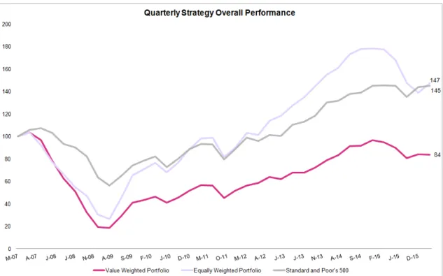
Figure 5 Overall performance (Quarterly Strategy) vs. Benchmark ... 27

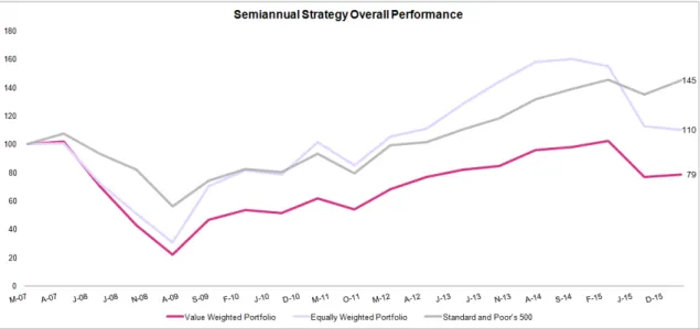
Figure 6 Overall performance (Semiannual Strategy) vs. Benchmark ... 27

Figure 7 Market tendencies definition (Quarterly Strategy) ... 28

Figure 8 Market tendencies definition (Semiannual Strategy) ... 29

Figure 9 Bullish Scenario (Quarterly Strategy) ... 29

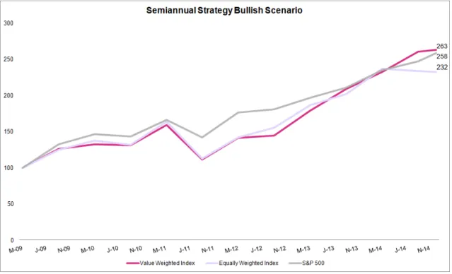
Figure 10 Bullish Scenario (Semiannual Strategy) ... 30

Figure 11 Overall performance based on worst stocks (Quarterly Strategy) ... 31

Figure 12 Overall performance based on worst stocks (Semiannual Strategy) ... 32

List of Tables

Table 1 Indexes Summary ... 16

Table 2 Summary results for overall period (Quarterly vs. Semiannual) ... 28

Table 3 Summary Results (Bullish Scenario) ... 30

Table 4 Summary Results (Stagnation Scenario) ... 31

Table 5 Summary results (upwards vs. downward revisions) - Overall Scenario and Quarterly Strategy ... 32

Table 6 Summary results (upwards vs. downward revisions) - Bullish Scenario and Quarterly Strategy ... 33

Table 7 Summary results (upwards vs. downward revisions) - Stagnation Scenario and Quarterly Strategy ... 33

Table 8 Summary results (upwards vs. downward revisions) - Overall Scenario and Semiannual Strategy ... 34

Table 9 Summary results (upwards vs. downward revisions) - Bullish Scenario and Semiannual Strategy ... 34

Table 10 Summary results (upwards vs. downward revisions) - Stagnation Scenario and Semiannual Strategy ... 35

(7)

1

1. Introduction

The inexistence of a single and “perfect” asset pricing model is one of the reasons behind the brilliance of the financial markets, in which investors can act based on their expectations.

In that sense, it is crucial to absorb all the available information you can, in order to make the right call. Automatically, some old questions arise: Are the financial markets reflecting efficiently the asset’s value through their price? Is there any discrepancy between the market price and its theoretical value during some time? Are prices reflecting all relevant information and, if not, how fast is it reflected into them?

The answers for these questions allow us to distinguish two alternative actions: active and passive management. The manager who believes in the market’s inefficiency will conduct an active strategy based on its own judgment in order to generate excess return. On the other hand, for those who believe that the market quickly absorbs all relevant available information, it will allow them to simply track the performance benchmark using, for instance, an index fund.

In order to test the efficiency of these two alternative investment strategies, we developed an active strategy by purchasing stocks selected from S&P 500 that experienced the highest three months’ revisions in their earnings by analysts. The study was conducted for a period of nine years and the two types of rebalancing the portfolios allow us to capture different market tendencies and to test the information absorption speed. Using different performance metrics, we will test if our strategy is capable to beat the market, which would represent the passive management strategy. We also applied the Fama and French model to check the existence of excess return.

(8)

2

2. Literature Review

2.1.Equilibrium models

According to the Modern Portfolio Theory, introduced by Markowitz (1952), a portfolio of assets should take into account the relationship between risk and return and should not look in perspective of individual assets. Markowitz proposed diversification as the way to reduce the total risk for the same level of return. Combining various assets, investors face a set of alternative portfolios associated with some kind of risk and return. Assuming normal distribution for the expected return probabilities, Markowitz states:

𝐸 𝑅_# = ) 𝑤_&𝐸(𝑅_&)

&*+ (1)

Where 𝐸 𝑅_# is the portfolio expected return, 𝑤_& and 𝐸(𝑅_&) are the weight of asset i in the portfolio and the return of asset i respectively. The variance of rate of return of the portfolio is given by:

𝑉𝑎𝑟 𝑅_# = ) 𝑤_&𝑤_/𝐶𝑜𝑣(𝑅_&, 𝑅_/)

/*+ )

&*+ (2)

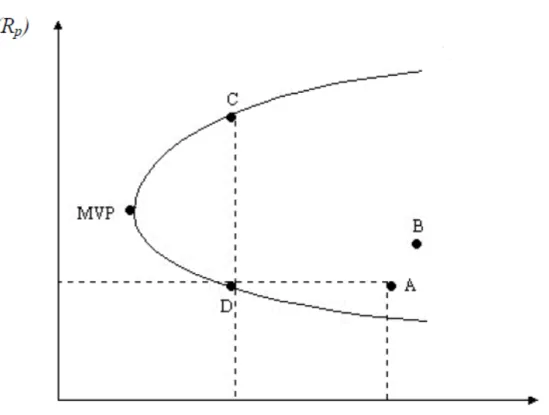
However, from all possible combinations, only few portfolios could be considered efficient because, for each level of return, only a single portfolio has a minimum variance (risk). Looking at figure 1, it is clear that a rational investor will only invest in a portfolio represented along the envelope line that starts at the dot MVP and goes up to infinite. The decision of which particular portfolio to select depends on the risk aversion of each investor. However, when there is the possibility of investing on risky free assets, either by lending or borrowing at the risk free rate, the efficient frontier changes to a straight line that starts at the risk free risk-return point and touches the risky envelope as

(9)

3

drawn in figure 2. Under this model, investors will combine the efficient risky portfolio with the riskless asset.

If investors act as above, then we are able to predict how the aggregate of investors will behave and how prices and returns are set in the market. The construction of general equilibrium models will help us to determine the relevant measure of risk for any asset as well as the relationship between risk and return for any asset when the markets are in equilibrium.

The first model called Capital Asset Pricing Model (CAPM) or the one-factor model was developed by Sharpe et al in 1960s and is obtained from the simplification of Markowitz’s model. Assuming that investors have homogeneous expectations and that the conditions showed in figure 2 hold, all investors will invest on the same risky portfolio, meaning that in equilibrium, all investors will take a position on the market portfolio. Individual differences will only reflect the investment weight in risk and risk-free assets, that is, an investment position throughout the capital market line. The equation for this straight line, which describes all efficient portfolios, is

𝑅₄ = 𝑅₅+7897:

;8 𝜎4 (3)

Where 𝑅₄ represents the expected return of the portfolio, 𝑅₌ denotes the expected return of the market, 𝑅₅ represents the risk free-rate, 𝜎₌ as a measure of risk of the market and 𝜎₄ as a measure of risk of the portfolio. However, this equation is not representative for the equilibrium of non-efficient portfolios or individual assets. Knowing that beta is the correct measure of risk for a well-diversified portfolio and that the market portfolio follows this condition, the only two dimensions that we need to

(10)

4

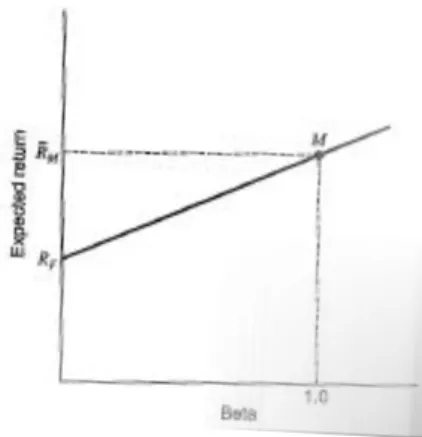
care are returns and beta. This relationship is presented in figure 3 and is called the security market line which describes the expected return for all assets and portfolios in the economy. The equation is given by

𝑅_& = 𝑅₅+ 𝛽_&(𝑅₌− 𝑅₅) (4)

Although the CAPM was used for decades, resulting in a Nobel Prize for Sharpe in 1990, Fama and French (1992) showed that the relationship between beta (the slope in the regression of a stock’s return on a market return) and average return was disappearing (1963-1990), not supporting the idea that average stock returns are positively related to market betas. Other authors found some contradictions in the Sharpe’s model. Banz (1981) has shown that market capitalization adds explanatory power to the cross-section of average returns provided by market betas. Bhandari (1988) got to the same conclusion adding the leverage effect. Fama cites that Stattman (1980) and Rosenberg, Reid and Lanstein (1985) found that the ratio of a firm’s book value of common equity to its market value is positively related to the average returns on US stocks. Additionally, Basu (1983) confirmed that earnings-price ratios help explaining the cross-section of average returns on US stocks with tests that included size and market beta. Between 1963 and 1990, Fama and French (1992) argued that the combination of size and book-to-market equity seems to absorb the roles of leverage and earnings-price ratio in average returns.

Later on, Fama and French (1993) extended the asset-pricing tests, essentially to expand the set of asset to be explained (like bonds) and adding term-structure variables to see if they play a role in bond returns. The goal of the authors was to see if the variables that mainly affect bond returns help to explain stock returns, and vice versa.

(11)

5

The authors found that the variation in stock returns is largely captured by three stock-portfolios returns, showing that a market factor and the proxy’s model for the risk factors related to size and book-to-market equity seem to help explain the cross-section of average returns. Based on these conclusions, we will explain the model behind our calculations for portfolios expected return.

The rationale behind Fama and French (1993) was to isolate the effects of each source of risk. The methodology followed was to construct six value-weighted portfolios which are built at the end of each June as a result of the intersection of two portfolios created based on size (ME) and three portfolios formed based on the ratio of book-to-market equity (BE/ME). The proxy for size is called SMB (Small Minus Big), that is, the average return on the three small portfolios minus the average return of the three big portfolios.

𝑆𝑀𝐵 =+_C 𝑆𝑚𝑎𝑙𝑙 𝑉𝑎𝑙𝑢𝑒 + 𝑆𝑚𝑎𝑙𝑙 𝑁𝑒𝑢𝑡𝑟𝑎𝑙 + 𝑆𝑚𝑎𝑙𝑙 𝐺𝑟𝑜𝑤𝑡ℎ −+_C(𝐵𝑖𝑔 𝑉𝑎𝑙𝑢𝑒 +

𝐵𝑖𝑔 𝑁𝑒𝑢𝑡𝑟𝑎𝑙 + 𝐵𝑖𝑔 𝐺𝑟𝑜𝑤𝑡ℎ) (5)

The other factor is called HML (High Minus Low) and it is used as a proxy for the book-to-market equity (BE/ME). It is the average return on the two value portfolios minus the average return on the two growth portfolios.

𝐻𝑀𝐿 =+_Q 𝑆𝑚𝑎𝑙𝑙 𝑉𝑎𝑙𝑢𝑒 + 𝐵𝑖𝑔 𝑉𝑎𝑙𝑢𝑒 −+_Q(𝑆𝑚𝑎𝑙𝑙 𝐺𝑟𝑜𝑤𝑡ℎ + 𝐵𝑖𝑔 𝐺𝑟𝑜𝑤𝑡ℎ) (6)

Lastly, the excess return on the market is given by 𝑅_R− 𝑅₅. Notice that we will briefly explain the construction of these portfolios later. Having these variables, we are able to predict asset returns using the formula below. The betas corresponded to the coefficients of each variable considering that 𝛽₌& _{is derived from CAPM.}

(12)

6

𝑅& − 𝑅5= 𝛼 + 𝛽=& 𝑅R− 𝑅5 + 𝛽T=U& 𝑆𝑀𝐵 + 𝛽V=W& 𝐻𝑀𝐿 (7)

2.2.Importance of EPS and analysts´ forecast

This research will focus on earnings per share (EPS) or, in detail, on the main impacts of earnings on prices and, in particular, on the role that the analyst estimates of EPS in the financial markets plays.

Several studies have shown that the reported earnings seem to have an effect on stock price movements. The tests conducted by Niederhoffer and Reagan (1972) allow us to conclude that stocks that perform well are those who have increased their earnings. This evidence will lead investors to act based on expectations, meaning that they will purchase stocks that create value for them (stocks that show high growth of EPS). If the market is efficient, then expectations about future earnings should be reflected on stocks prices and investors should not be able to gain excess returns based on consensus expectations about future earnings. We can now introduce the role of analysts’ earnings forecast. They can be used (1) as proxies in valuation models to forecast future share prices, e.g. discounted cash flows method; (2) to analyze the effect of surprise level (difference between actual reported earnings and analysts’ earnings forecasts); (3) to examine if security returns follow the market efficiency theory; and (4) as a source of information for market participants.

Gleason and Lee (2003) state that individual analysts´ forecast revisions play an important role in the dissemination of information about corporate earnings. They are also important in changing investors’ decisions and investment strategies. As new information becomes available, analysts revise their EPS estimates and investors can act based on these revisions in order to earn large excess returns. However, that information

(13)

7

adjustment is slowly absorbed by the market, meaning that market participants do not immediately assimilate certain potentially qualitative aspects of an earnings´ signal. Gleason and Lee (2003) found that the market does not make a sufficient distinction between revisions that provide new information and revisions that merely follow the consensus. Additionally, they found that the price adjustment process is faster and more complete for ‘celebrity’ analysts. This is in line with the findings of Elton et al. (1981), which found that an investor could earn excess returns by doing a better revision than consensus. As a result, an investor can benefit, making abnormal returns, because some analysts seem to perform better than others. However, analysts can be encouraged to report optimistic earnings due to conflicts of interest generated by investment banking relationships. In response, investors may adopt a cynical posture and use a wait-and-see approach when it comes to good news, as McKnight and Todd (2006) reported. This evidence is in line with Hong et al. (2000) that made a distinction between the market reaction to good and bad news, concluding that the first ones travel slowly in contrast to the quickness of bad news.

2.3.Some results of EPS revisions

The majority of works regarding the possibility of earn excess return according to estimates of EPS revisions refer to Elton et al. (1981) paper. Collecting firms that have fiscal years ending on December 31 and that are followed by three or more analysts, Elton et al. (1981) took a sample of 913 one-year earnings forecasts and 696 two-year earnings forecasts on March and September of each year (1973 to 1975). In general, March is the earliest date in which most companies report their financial results and September is the date that is far enough from the first forecast and far enough from the last firm report. Additionally, firms that experienced negative earnings at some time

(14)

8

were excluded from the sample. Considering portfolios with a holding period of 24 months, the authors concluded that the largest returns can be earned by selecting stocks for which analysts make the most significant revisions in their estimations. Based only in the consensus estimation of EPS, investors should not be able to earn excess returns due to the fact that all relevant information is already included in share prices. However, the authors found that it is possible to earn excess returns by selecting stocks which analysts had underestimated returns. In other words, the foreknowledge of analyst revisions is more value-relevant than the reported earnings themselves. It is important to note that excess return is defined here as the difference between actual return and expected return, based on the market model.

These results are consistent with those of Benesh and Peterson (1986). Between 1980 and 1981, the authors split the sample for each year into three subsamples, consisting of: (1) the 50 firms with the highest realized returns during the year; (2) the 50 firms with the worst realized returns during the year; and (3) the reaming firms. The stock selection was based on firms that (1) have a December fiscal year, (2) are followed by three or more analysts and (3) have monthly data available about earnings and forecasts. According to the authors, stocks that are subject to significant revisions (more than 5%) on their earnings during the first two quarters of the year, tend to lead to significant excess return over the remainder of the year. Additionally, analysts’ revisions of their forecasts become more optimistic as time passes for the eventual top-performing firms and more pessimistic for the worst firms.

In our research we will follow a similar approach to Hawkins et al. (1984). These authors refined the ideas of Elton et al. (1981) searching on how to earn excess return by predicting changes in the consensus estimate. The authors constructed equally

(15)

9

weighted quarterly portfolios between March 1975 and December 1980. They were able to create portfolios consisting of 20 stocks with the largest one-month increase in the consensus earnings estimate. The tests are consistent with the earlier findings. It is possible to achieve returns significantly above the market’s return, even if we take risk adjustment returns or different holding periods into account.

These results are in accordance with early research by Griffin (1976), Givoly and Lakonishok (1979 and 1980), and Imhoff and Lobo (1984), who have concluded that the market seems to react to analyst forecast revisions. Stickel also (1991) demonstrated that investing in firms whose consensus forecast has been recently revised upward lead to abnormal returns over the next 3 to 12 months, contrary to those whose consensus has been revised downward.

All these studies seem to disagree with the idea that markets are efficient according to Fama (1970).

3. Data

Our database covers the nine years period of between January 2007 and December 2015. We created a monthly database with 12 months forecast EPS given by the average market consensus for each stock which belongs to the S&P 500 in the observation month. This time frame was selected in order to capture different market moments (bull, bear or stagnation) and the use of 12 months forward EPS allows us to include stocks with a fiscal year that does not end in December, making all stocks comparable in our universe. Our filter was based on the exclusion of stocks that were not followed by, at least, three or more analysts or stocks that have negative forecast EPS. All this data was collected from Bloomberg.

(16)

10

We used the Fama and French (1993) model to compute assets’ expected returns in order to compare them with observed returns. As we have mentioned before, the variables from the model are based on the creation of six value-weight portfolios, which results from the intersections of two portfolios based on size (market equity, ME) and three portfolios based on the book to market equity ratio (BE/ME). The size breakpoint for year t is the median NYSE market equity at the end of June of year t. BE/ME for June of year t is the book equity for the last fiscal year end in t-1 divided by ME for December of t-1. The BE/ME breakpoints are the 30th and 70th NYSE percentiles (figure 4). The portfolios from July of year t to June of t+1 include all NYSE, AMEX and NASDAQ stocks for which we have market equity data for December of t-1 and June of t, and (positive) book equity data for t-1. Instead of creating our portfolios using this procedure in order to find SMB, HML and Rm- Rf, we will move forward and use the

results from the authors’ data library available at

(17)

11

4. Methodology

This paper is based on the idea that it is possible to observe abnormal returns by creating an investment strategy based on stocks with the three months’ highest upward revision in their EPS. This includes two different strategies:

• The one that selects stocks with the highest three-month EPS revision and a quarterly holding period.

• Another that selects socks with highest three-month EPS revision and a semiannual holding period.

The reason for using different holding periods relates with the time of the market reaction of the event under scope or, in other words, to how the market accommodates this type of information. In addition, we want to test whether there are differences in the market reaction according to different market trends. Therefore, we split our sample in order to pick up different market tendencies and see the strategy behavior:

• Bear market – between March, 07 and February, 09

• Bull market – between March, 09 and December, 14

• Stagnation – between January,15 and March,16

Sometimes the EPS revisions are limited and just seem to follow an optimism in the market. With longer EPS revisions, more information is available for analysts and the estimates become more realistic and noticeable for investors.

The metric that we use concerning the estimated earnings per share is the forward twelve-months, given by the average consensus of analysts. Let´s suppose that we are at

(18)

12

the beginning of March 2009 and want to analyze a company whose fiscal year ends in May 2009. The estimated EPS 12F for that month will contemplate about 17% of the estimated EPS for 2009 and the remaining for the next fiscal year. As we have mentioned before this metric will allow us to include companies that do not have a fiscal year ending in December.

The first step of our work was to collect the S&P 500 index composition at each month. Next, we got the monthly analysts’ projection for each index member during our analysis period.

Having the forecasts, we estimated the percentage of revision for each stock and for each revision. We excluded stocks that were followed by less than three analysts or stocks that had negative earnings for any observed month. Applying this filter, we rated it based on the highest percentage revision.

Depending on the strategy (quarterly or semiannually), we created portfolios composed by the twenty stocks that experienced the highest analysts’ estimated EPS revision. For our analysis, we will take into consideration equally weighted portfolios and market-capitalization weighted portfolios, in order to minimize the risks of including small stocks, which are historically riskier.

The weights were estimated at the beginning of the portfolio creation and were kept constant during the holding period. In each purchased period, we formed a capitalization-weighted index with twenty members selected from the portfolio, in order to get the required weights. The weight to invest in each stock is given by:

𝑤& = =XYZ4[ \X#_=XYZ4[ \X#]

] ^_

(19)

13

Where Market Capi stands for each stock and Qd_&*+𝑀𝑎𝑟𝑘𝑒𝑡 𝐶𝑎𝑝_& represents the total

market capitalization of the portfolio. In the end, we were able to compute the observed returns which are given by the individual returns by taking their weights in the portfolio into account.

𝑅_# = Qd 𝑥_&𝑅_&

&*+ (9)

Where 𝑅_# is the portfolio return, 𝑥_& 𝑅_& are the weight and return of asset i.

Regarding the two different strategies, the observed returns of each portfolio were then subject to some performance metrics, in order to test if the strategies would lead to earn any excess return (risk-adjusted alpha), beating the market. We define alpha as the difference between the portfolio return and market absolute return or the expected return, given by the Three Factor Model.

𝛼_# =7f

gf− 𝑅h (10)

𝛼# = 𝑅#− 𝑅# (11)

We also perform the Sharpe Ratio (1966), Information Ratio and Sortino Ratio (1994). 4.1.Some considerations

As the S&P500 index does not incorporate dividends on its calculation, we also discarded their effect on prices, particularly their reinvestment. Besides the fact that the dividends would improve the results of our performance strategy, their absence will make the results directly comparable with the benchmark. Stock prices were adjusted for any change in capital equity structure (e.g. mergers & acquisitions and spin-offs) and in the stock price itself (e.g. reverse stock split). When there was a loss of a

(20)

14

portfolio member in a certain holding period, the portfolio was kept until maturity, with the remaining components.

4.2.Performing measures Sharpe Ratio

The Sharpe Ratio (SR) developed by William F. Sharpe (1966) has the aim to measure risk adjusted return. Originally, the SR was designed as forward-looking ratio, in order to determine what reward an investor could expect for investing in a risky asset, instead of investing in a riskless one. Throughout the years, portfolio managers began to employ it by using actual returns. The SR is calculated by subtracting the average return of the risk free rate from the average return of the portfolio and dividing that difference by the average standard deviation (volatility) of the portfolio. In order words, it represents the excess return earned per unit of volatility, meaning that no matter if a portfolio reaped higher returns than it is peers but, how much additional risk is added to achieve that return. A negative ratio indicates that a riskless asset would perform better than the security being observed.

𝑆𝑅 =7f97i

;f (12)

The risk measure, given by the standard deviation, was based on historical information.

We performed this metric for all portfolios and for the benchmark during each period time (quarterly or semiannually).

(21)

15

The Information Ratio (IR) is another measure for the risk adjusted return and it is referred to as a generalized version of the SR. It tells us how much excess return is generated from the amount of excess risk taken relative to the benchmark. This IR is used for measuring active management managers against a passive benchmark. Like SR, the IR is based on the Markowitz mean-variance assumptions.

𝐼𝑅_# = 7f97k

lm (13)

Where TE (Tracking Error) tracks how a portfolio replicates the benchmark. It is the standard deviation of the difference in returns between the portfolio and its benchmark.

𝑇𝐸 = 𝑉𝑎𝑟(𝑅_#− 𝑅_R) (14)

A portfolio manager who wants to replicate the benchmark, looks for a TE close to zero.

Using the Sharpe Ratio allow investors to compare funds by taking their risk tolerance into account in order to see which funds have the best risk adjusted returns. On the other hand, the Information Ratio is used to rank manager performance.

Indexes performance

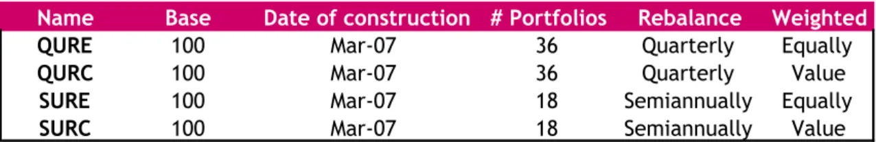
We proceeded with the creation of four indexes regarding the two different strategies (quarterly or semiannual holding period) and the index construction type (equally weighted or value weighted). This will allow us to easily check different performances and take some conclusions over the study period.

(22)

16

Table 1 Indexes Summary

The portfolios consisted in 20 stocks that showed the highest 3-months’ revision in the EPS estimate. The initial purchases are assumed to be made at the end of March 2007 and, depending on the strategy, to be rebalanced quarterly or semiannually. At the end of March 2007 (t=0) the indexes start at an initial level of 100 points. At time t the index value (I) is computed as:

𝐼_[ = 𝐼_[9+×(1 + 𝑅_[9+) (15)

in which the 𝑅_[9+ is the portfolio return at time t purchase at time 𝑡 − 1. Please read the methodology section to note the considerations about the portfolio construction.

Fama and French (1993) Model

Using a Confidence Interval of 5%, we run a multiple linear regression with 10 years historical data in order to estimate betas at the corresponding portfolio purchase period. The parameters’ estimation includes the last year average observed data, collected by Fama’s website.

4.3.Error types

Essentially, we can distinguish four types of bias regarding the creation of an investment strategy based on quantitative methods:

• Data Mining Bias – researchers use historical data as an attempt to find significant patterns and try to predict how the population will behave in the

Name Base Date of construction # Portfolios Rebalance Weighted

QURE 100 Mar-07 36 Quarterly Equally

QURC 100 Mar-07 36 Quarterly Value

SURE 100 Mar-07 18 Semiannually Equally

(23)

17

future. Any conclusion can be potentially useful but many others might just be coincidental and may not be repeated in the future, especially if we assume the efficiency market hypothesis.

• Look Ahead Bias – occurs when estimated data is used at the testing period. The majority of our project decisions are based on historical price series. However, the use of Fama and French (1993) model implies the use of some estimated data regarding the factors derived from the model.

• Time-period Bias - refers to a study that may appear to be successful only in certain periods. This is the reason why we chose the time range between January 2007 and December 2015 with the aim to pick up different market tendencies (bull and bear market).

• Survivorship Bias – results when an index member is not included in the basket due to its bankruptcy or other capital structure change, or because of its exit from the S&P500 index. Taking this into consideration, we filter the stocks that composed the index at each purchase period. As we have mentioned before, if any stock is discarded during any holding period, the portfolio return will be based on the last information available, even if their composition is less than 20 stocks at maturity.

5. Empirical Results

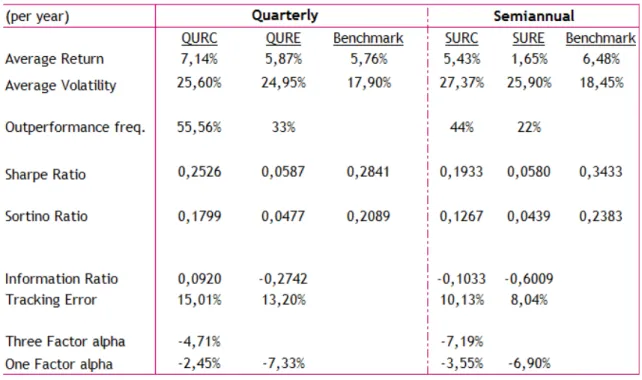
In general, our strategy was unable to beat the market. In March 2007, investing in our market value weighted portfolios could represent an accumulated gain of about 25% (in case of quarterly portfolios) and 4% (considering semiannual strategy) during the 9 years period (See Figures 5 and 6). These results are quite disappointing when looking

(24)

18

into what a passive strategy of investing on the S&P500 achieved. The benchmark accumulated about 45%, facing much lower volatility than the QURC and SURC indexes. The higher Sharpe measure from benchmark allow us to prefer investing in S&P 500. Both indexes represented an average negative annual alpha, in accordance with our estimates with the Fama and French (1993) Model. About 56% of the QURC index portfolios outperformed the benchmark. This percentage reaches 44% if we analyze semiannual rebalancing frequency. See table 2 for the main results.

The definition of market tendencies allowed us to find different patterns during a bear, bull and stagnation period. It is clear that when the market faces a correction, our strategy suffers a higher pressure, with significant losses compared with the benchmark (Figures 7 and 8). This statement is in accordance with our Sortino results, in which the majority of all scenarios represented a smaller performance compared with the S&P500 returns. On the other hand, any bullish moment seems to accelerate it. During the big optimistic period between March 2009 and December 2014, both market-value weighted indexes had outperformed the S&P500 by 37.7pp (quarterly strategy) and 4.6pp (semiannually strategy) in absolute terms and generated higher average annual returns. However, due to the lower volatility, the benchmark had a better risk-adjusted return with a Sharpe Ratio of 1.281, which compares with the 1.061 and 0.918 from the QURC and SURC indexes, respectively. The conclusions are similar to what we described before for the entire range sample, suggesting that the risk exposure to the QURC and SURC indexes do not compensate the investor. The outperform frequency closes to 50% in both indexes, generated a negative average alpha of about 2pp, opposite to our estimations using the Fama and French (1993) Model. See figures 8/ 9 and table 3 for the main results.

(25)

19

When the market faces a stagnation period, the results from the QURC index performance are quite relevant. The index has outperformed the benchmark in terms of absolute and risk-adjusted return. Between January 2015 and March 2016, the QURC index has accumulated about 11% with a Sharpe Ratio of 0.49, which compares with the SR of 0.02 from the S&P500. The index outperformed the benchmark 60% of time, and generated an excess annualized alpha of 13,14pp. This excess of return suggests that active management is preferable when the market faces a flat market period, which in this case is coincident with the suspension from the US Federal Reserve regarding the QE program and given the low economic growth prospects. Additionally, about 60% of the portfolios have outperformed the benchmark in terms of risk-adjusted return. See table 4.

Our results have shown that the equally-weighted indexes did not bring any additional benefit to investors, since those indexes have underperformed against the value-weighted indexes for all scenarios and measures.

As we predicted, the rebalancing frequency reduction seems to have an impact in our strategy. In all the scenarios, the use of semiannual rebalancing period appears to diminish our performance. This conclusion is in accordance with the market efficiency hypothesis, which states that the information disclosure to the market is quickly absorbed. Our results are in accordance with the ones of Plyakha et al. (2014) that found the same results we did, except during the bull market. The authors found that the reduction of the rebalancing frequency leads to a reduction of the alpha. Bearing the entire sample in mind, the QURC index has produced on average an annualized alpha of -2.45pp against a negative effect of 3,55pp from the SURC index. The difference is even bigger when we consider our best scenario (the stagnation period). The same

(26)

20

analysis can be conducted if we compare the market value weighted indexes with the equally weighted indexes.

Although the IR allows us to compare our strategies, evaluating them in a world where there are so much active managers is challenging. Some research has been done in order to distinguish the different levels of IR. According to Kahn (2000), top-quartile active equity managers have information ratios of 0.50 or higher. Grinold and Kahn (1995) defined an IR of 1.0 as “exceptional”, 0.75 as “very good” and 0.50 as “good”. However, the consensus from the professionals shows that an IR between 0.20 and 0.30 is superior. Looking at our strategies, only two funds fulfill the requirements:

• QURC index during the bullish period

• QURC index during the stagnation period

Note that this conclusion confirms what we have stated before: the use of market value weighted portfolios added to higher rebalancing frequency leads to better results.

Believing on market's overreaction, we tested the same procedure for stocks that have been revised down. In fact, equally-weighted portfolios have performed well compared with our best strategy designed before, signalizing a positive contribute from small firms. Considering the entire sample, the QURE index has generated an average positive alpha of 10bp (vs. -7.33pp), with 56% of the total portfolios outperforming the benchmark. These results are improved under the bullish scenario, where the QURE index had an accumulated gain of more than 500%, facing much lower volatility than the comparable index. Additionally, almost 80% of the portfolios have outperformed the

(27)

21

benchmark, and generated an average alpha of about 12pp. Like the first one, this strategy seems to be smashed by bear and stagnation periods.

In this case, introducing market-value weighted portfolios does not bring any additional benefit for the investor, and increasing the rebalancing frequency seems to diminish the performance, in accordance to what was found above. See tables 5 to 10 and figures 11 and 12 to observe these conclusions.

6. Conclusion

Managers and investors have long shown an appetite to beat the market. some active strategies have indeed demonstrated the ability to create excess return but the higher volatility seems to diminish their performance, in accordance with Markowitz’s theory. In this framework and taking advantage of Hawkins’s studies, a new active investment strategy in the US stock market was proposed based on changes in analysts’ expectations. Considering the entire sample, the strategy was not capable to beat the market. However, it seems to behave differently when it faces different market tendencies, especially in a bull and stagnation period.

In some activity sectors, the use of EPS seems to have a little impact on market reactions since there are other measures that replicate better the sector performance (e.g. evolution of NPLs for the banks and margins for retail). In that sense, would be relevant to substitute the EPS measure in our work to other such as sales, margins, operating costs, etc.

(28)

22

This paper assumes that the information available is released at the same time. In fact, the analyst projections are known progressively during a month and should be interesting for future works to design portfolios according to that timing.

7.

Bibliography

Benesh, Gary A. and Peterson, Pamela P. (1986). On the Relation Between Earnings, Changes, Analysts’ Forecasts and Stock Price Fluctuations. Financial Analysts Journal 42 (6), 29-39, 55

Elton, Gruber, Martin J. and Gultekin M. (1981). Expectations and Share Prices. Management Science 27 (9), 975-987

Elton, Gruber, M., Brown, S. and Goerznann, W. (2014). Modern Portfolio Theory and Investment Analysis. 7th edition. New York: John Wiley & Sons

Fama, Eugene F. and French, Kenneth R. (1992). The Cross-Section of Expected Stock Returns. The Journal of Finance 47 (2)

Fama, Eugene F. and French, Kenneth R. (1993). Common risk factors in the returns on stocks and bonds. Journal of Financial Economics 33, 3-56

French, Kenneth R. (2016). Available at:

http://mba.tuck.dartmouth.edu/pages/faculty/ken.french/index.html

Givoly, D. and Lakonishok, J. (1979). The information content of financial analysts’ forecasts of earnings. Journal of Accounting and Economics 1, 165-185

(29)

23

Gleason, Cristi A. and C. Lee, Charles M. (2003). Analyst Forecast Revisions and Market Price Discovery. The Accounting Review 78 (1), 193-225

Griffin, P. (1976). Competitive information in the stock market: An empirical study of earnings, dividends, and analysts’ forecasts. Journal of Finance 31, 631-650

Grinold, R. C. and Kahn, R. N. (2000). Active Portfolio Management. McGraw-Hill, New York, second edition

Hawkins, Chamberlin, Stanley C. and Daniel, Wayne E. (1984). Earnings Expectations and Security Prices. Financial Analysts Journal 40 (5), 24-38, 74

Hong, Lim, T. and Stein J. (2000). Bad News Travels Slowly: Size, Analyst Coverage, and the Profitability of Momentum Strategies. Journal of Finance 55 (1), 265-295

Imhoff, E. and Lobo, G. (1984). Information content of analysts’ composite forecast revisions. Journal of Accounting Research 22, 541-554

Markowitz, H. (1952). Portfolio Selection. The Journal of Finance 7 (1), 77-91

McKnight, Phillip J. and Todd, Steven K. (2006). Analyst Forecasts and the Cross Section of European Stock Returns. Financial Markets, Institutions & Instruments 15 (5), 201-224

Niederhoffer, V. and Regan, Patrick J. (1972). Earnings Changes, Analysts’ Forecasts and Stock Prices. Financial Analysts Journal 28 (3), 65-71

Plyakha, R. Uppal, and G. Vilkov (2014). Equal or Value Weighting? Implications for Asset-Pricing Tests. SSRN

(30)

24

Sharpe, William F. (1964). Capital Asset Prices: A Theory of Market Equilibrium under Conditions of Risk. The Journal of Finance 19 (3), 425-442

Sharpe, William F. (1966). Mutual Fund Performance. The Journal of Business 39 (1), 119-138

Sortino, Frank A. and Price, Lee N. (1994). Performance Measurement in a Downside Risk Framework. The Journal of Investing 3 (3), 59-64

Stickel, Scott E. (1990). Predicting Individual Analyst Earnings Forecasts. Journal of Accounting Research 28 (2), 409-417

(31)

25