A statistical learning in chip-based test and diagnostics methodology

(1)

F

ACULDADE DE

E

NGENHARIA DA

U

NIVERSIDADE DO

P

ORTO

A Statistical Learning in Chip-based

Test and Diagnostics Methodology

César Carpinteiro

Mestrado Integrado em Engenharia Eletrotécnica e de Computadores

Supervisor: José Machado da Silva Second Supervisor: R. D. (Shawn) Blanton

(2)

c

(3)

(4)

(5)

Resumo

À medida que a indústria dos circuitos integrados alcança capacidade de fabrico de semicondutores de dimensões nanométricas, os circuitos ficam mais vulneráveis a mecanismos de envelhecimento que começam por se manifestar como atrasos de propagação crescentes, levando à redução da vida útil dos circuitos. O recurso a bandas de guarda, isto é, bandas de tolerância mais largas, é uma das soluções adotadas para melhorar a fiabilidade do circuito, mas esta prática torna o custo final mais oneroso. Sistemas de aprendizagem estatística têm sido desenvolvidos para inferir o ponto ótimo de operação do circuito a partir de dados de stress recolhidos e assim evitar sobredi-mensionamentos. Em particular, a metodologia CASP testa o circuito a frequências mais elevadas para detetar falhas iminentes. Esta metodologia de diagnóstico permite localizar falhas ao nível do sub-circuito, ainda que com alguma ambiguidade. Algoritmos de aprendizagem podem ser usados para melhorar a exatidão da deteção e localização.

Neste trabalho vários algoritmos de aprendizagem foram analisados para melhorar a precisão do diagnostico do CASP. A abordagem baseada no algoritmo Dynamic K-Nearest Neighbors mostrou ser a que apresenta melhor desempenho. O classificador DKNN foi implementado usando matrizes sistólicas de modo a obter uma solução completamente parameterizável, que alcança lin-earidade temporal e de utilização de recursos. Esta solução foi sintetizado para implementação em FPGA com uma utilização mínima de recursos e um tempo de execução competitivo.

(6)

(7)

Abstract

As the integrated circuits industry reaches the capability of fabricating semiconductors with nano-metric features, circuits become more susceptible to aging mechanisms, which start to manifest as increasing propagation delays, leading to a reduction of circuits lifetime. Resorting to design guard bands, that is larger tolerance bands, is one of the solutions that has been adopted to im-prove circuit reliability, but this practice comes at the cost of more expensive production costs. Statistical learning engines are being developed to infer the optimum operating point of a circuit from gathered stress data and thus to avoid costly overdesign. In particular, the CASP methodol-ogy tests a circuit at an higher frequency to detect looming failures. This diagnostic methodolmethodol-ogy pinpoint failures at the sub-circuit level, yet with some ambiguity. Machine learning algorithms can be used to improve the accuracy of the fault detection and localization.

In this work several machine learning algorithms were analyzed in order to improve accuracy of CASP diagnostic. The approach based on the Dynamic K-Nearest Neighbors showed to be the one that ensures the best performance. The DKNN classifier was implemented with a systolic array architecture in a fully parameterizable design which shows both temporal and resource us-age linearity. The design was synthesized for implementation in a FPGA platform with minimal resource usage and competitive execution time.

(8)

(9)

Agradecimentos

Há 5 anos atrás lá comecei eu indeciso a minha caminhada para me tornar engenheiro. Hoje só me arrependo que não tenha durado mais tempo. Nestes anos cresci muito como pessoa e estudante, fiz grandes amizades, descobri novas paixões e tive a oportunidade de conhecer um pouco desse vasto mundo.

Em primeiro lugar quero agradecer à minha Família por sempre acreditarem em mim e tornarem tudo isto possível. Tudo o que sou - defeitos, virtudes, sonhos, objectivos - devo aos meus pais e é com um profundo orgulho e gratidão que guardo todos os vossos conselhos, reprimendas e carinho. À minha irmã agradeço todas as nossas guerras insignificantes, alianças contra os pais e conversas aleatórias. De ti só espero excelência e tenho imenso orgulho em ser teu irmão.

Esta dissertação não seria possível sem todo o apoio dos meus orientadores. Ao Prof. José Machado da Silva agradeço todo o apoio e conselhos que me deu, bem como toda a preocupação que teve comigo. Ao Prof. Shwan Blanton fico grato pelo acholhimento excelente que me deu nos Estados Unidos e nunca vou esquecer as nossas conversas sobre doutoramento. Ao Xuanle Ren quero agradecer toda a assistência que me deu para tornar esse trabalho possível.

Um curso é tão bom quanto os seus professores e eu tenho muito que lhes agradecer. Em particular tenho de referir os Professores Pedro Guedes Oliveira, João Barros, Jaime Cardoso e Paulo Sá não só pôr serem excelentes professores, mas sobretudo por me aturarem e me darem uma visão nova do mundo.

Uma vida não se faz sem amigos e eu devo ter os melhores, já que me conseguiram suportar durante todo este tempo. Aos meus amigos desde sempre Sara, Zé Barbosa e Gonçalo obrigado por todas as conversas debaixo das estrelas, aos churrascos e as caminhadas. Ao Miguel por estares ao meu lado quando eu precisei, nunca me esquecerei. E também ao Vítor, Fábio, Vilaça, Tiago e Rafa, por maior que seja a distância quero voltar ao Plátano e econtrar-vos sempre lá.

A todos os amigos que fiz na faculdade, em especial o Diogo e o Vinícius, espero que me protejam das árvores e não me deixam transformar em Jesus Cristo. À Team CMU que descobriu os segredos da black magic conto convosco, Bernardo, Xico e João para destrocar pesado nos 50 estados.

Tenho grandes recordações de Delft e de toda a gente fantástica que lá conheci. Com Manel, André e João, criamos os Sons of Kapsalon, escrevemos os mandamentos do Kapsalon e vimos a encarnação da mitica Fénix.. Vou ter saudades. Foi também em Delft the que conheci a menina grega mais atrasada do mundo. Marianthi, obrigado por me fazeres tão feliz e por aturares um português tão irritante. A distância é grande, mas eu tenho um plano.

(10)

(11)

Acknowledgments

Five years ago there was I unsure in my quest to become an engineer. Today, my only regret is that it didn’t last for longer. In these years I grew up a lot as an person and as a student, I made great friendships, I discovered new passions and had the opportunity to know a little from this vast world.

In first place I want to thank my Family for always believing in me and making all this possible. Everything I am - defects, virtues, dreams and goals - I owe it to my parents and it’s with a deep pride and gratitude I save all your advice, rebukes and affection. To my sister I thank all our insignificant wars, alliances against our parents and random talks. I only expect excellence from you and I have a huge pride in being your brother.

This dissertation wouldn’t be possible without all the support from my supervisors. To Prof. José Machado da Silva I thank all the support and advice he gave and the general concern he always had for me. To Prof. Shawn Blanton I’m grateful by excellent reception he gave when I was in the United States and I will never forget our talks about PhD. To Xuanle Ren I want to thank all the help he provided me to make this work possible.

A master is as good as its professors and I have much to thank to them. In particular, I need to refer professors Pedro Guedes Oliveira, João Barros, Jaime Cardoso and Paulo Sá not only for being excellent teachers, but most of all for putting in up with me and giving me a new vision of the world.

A life is not made without friends and I must have the best of them, since they stick around me for all this time. To my friends since the beginning Sara, Zé Barbosa and Gonçalo thank you for all the conversations under the stars, the barbecues and the hikes. To Miguel for being there when I needed, I will never forget. And also to Vítor, Fábio, Vilaça, Tiago and Rafa, the distance can be huge but I want to return to Plátano and find you all always there.

To all my friends I made in faculty, in special Diogo and Vinícius, I hope you protect me from trees and don’t let me transform in Jesus Christ. To Team CMU which uncovered the mysteries of the black magic I’m waiting for you, Bernardo, Francisco and João to "destrocar pesado" in the 50 states.

I have the best memories from Delft and all the great people I’ve meet there. With Manel, An-dré and João, we created the Sons of Kapsalon, wrote the commandments of the Mighty Kapsalon and watched to the incarnation of the mythical fenix.. I will miss you. It was also in Delft I’ve meet the most delayed greek girl in the world. Marianthi, thank you for making me so happy and for putting up with this annoying portuguese. The distance is great, but I have a plan.

(12)

(13)

“A sorte protege os audazes”

(14)

(15)

List of Figures

2.1 Transistor cross sections illustrating negative-bias temperature instability (NBTI) (a), HCI (b), RTN (c), and TDDB (d). Positive-bias temperature instability (PBTI) is equivalent to NBTI but occurs in an n-channel metal oxide semiconductor (NMOS)

device [1] . . . 4

3.1 Fault Dictionary Structure . . . 12

3.2 (a) The Pass/Fail (PF) test response register stores test responses in a circular buffer, (b) the fault accumulator (FA) tracks faults compatible with observed in-correct behavior, and (c) the faulty module identification circuitry (FMIC) maps faults, tracking how many compatible faults are within each sub-circuit [2]. . . . 13

3.3 Error rate of the DKNN classifier for increasing training set sizes. . . 17

3.4 Error rate of the DKNN classifier for increasing neighborhoods. . . 18

4.1 KNN Dependency Graph. . . 20

4.2 DKNN Signal Flow Graph. . . 21

4.3 The Xilinx Zynq-7000 ZC706 Evaluation Kit. . . 25

(18)

(19)

List of Tables

3.1 Mean percentual error rate and standard deviation for static and dynamic data. . . 16

4.1 Execution time (ms). . . 28

(20)

(21)

Abbreviations e Symbols

BTI Bias Temperature Instability

DKNN Dynamic K-Nearest Neighbor ELF Early Life Failure

FF Flip-Flop FIFO First In First Out

FPGA Field Programmable Gate Array HCI Hot Carrier Injection

ILP Instruction Level Parallelism IP Intellectual Property

KNN K-Nearest Neighbor

MOSFET Metal-Oxide-Semiconductor Field Effect Transistor N-LUT N input Lookup Table

PE Processing Elements RAM Random Access Memory RTN Random Telegraph Noise SoC System-on-Chip

SVM Support Vector Machine

(22)

(23)

Chapter 1

Introduction

As the semiconductor industry continues to scale down to 1X nm geometry features, variations occurred in the fabrication process have a higher impact on overall transistor dimensions. Fur-thermore, the devices become more susceptible to aging mechanisms such as bias temperature instability (BTI), hot carrier injection (HCI), random telegraph noise (RTN), and other physical and chemical phenomena occurred in the circuits structures — metal-oxide semiconductor (MOS) transistors and interconnections. These flaws manifest as different performance deviations of the circuits’ behaviors, being increasing propagation delays observed over the circuits’ lifetime one of the most critical ones, as far as their detection is concerned.

The designer’s job is to guarantee the system will operate correctly despite the various types of misbehaviors. One approach is to overdesign the circuit to operate at a higher than required speed to cope with the variability of the manufacturing process and device aging effects. A designer can also improve fault tolerance after replicating functional units or repeating operations during execution. However, such approaches result in significant performance losses, extra area over-head, and excessive power consumption, which are unacceptable for many embedded and energy constrained devices.

Since performance variations are increasingly harder to control, one can tackle the problem by accepting the unique characteristics of each device. In chip learning engines rely on stress data, usage patterns and error detection data to infer the device state and tune operating parameters to achieve optimal performance. Sensors spread through the chip can be used to reliably detect aging defects. A learning engine can mitigate those effects by reducing the operating voltage and frequency of the stressed area of the chip or reduce the execution load in the case of a multi-processor system. These are means that can be explored to allow potentially defective circuits to heal or to delay the degradation process.

Another way to detect defects is to periodically stop the system and test the circuit (off-line test), using high coverage test vectors. The output vectors are matched against a fault dictionary to narrow down the identification of possible locations of the defective component. To detect failures

(24)

2 Introduction

modern designs use several terabytes of space.

Regarding the availability problem, one solution that has been proposed is the CASP method-ology. The in chip CASP controller schedules a core of the chip for testing, while the remaining cores maintain their normal mission operation. After matching the core under test (CUT) output response with the fault dictionary data present in an off chip memory, repair or replacement of the faulty core (or sub-circuit) is done. The fault dictionary not always pinpoints just one sub-circuit and thus CASP can wrongly repair a non-faulty sub-circuit.

To improve accuracy of the faulty module prediction, machine learning algorithms can be used. Dynamic k-Nearest Neighbor uses the CASP diagnosis results as input and provides a prediction of the most likely faulty core making use of previously defined correctly labeled training data. Dynamic kNN can update the training data to gradually adapt to new fault patterns.

The work presented in this dissertation had two main goals: in the one hand, the evaluation of different machine learning based algorithms aiming to improve the accuracy of online failure detection in digital circuits. The algorithms were trained with fault data of a simulated cache controller, which revealed the DKNN classifier was the best performing choice; and on the other hand, redesign the hardware architecture proposed in [3] for the DKNN classifier and implement it for the first time in a FPGA target. Additionally, relevant performance results are presented and implementation considerations are made which support that the lean and fast hardware design proposed is suitable to a low impact silicon implementation.

Support for this research was provided by the Fundação para a Ciência e Tecnologia (Por-tuguese Foundation for Science and Technology) through the Carnegie Mellon Portugal Program.

1.1 Dissertation Structure

After this introduction, this dissertation continuous, in chapter 2, by providing an overview of circuit aging mechanisms in MOS circuits, detection sensors and testing methodologies to detect faulty behaviors caused by said mechanisms and some fault tolerant systems implemented to mit-igate aging. In chapter 3 a comparison is made among several machine learning algorithms to justify the choice of the DKNN classifier. Chapter4 describes the hardware architecture of the DKNN based classifier and the posterior implementation in FPGA. Results from the FPGA im-plementation are provided. Chapter5summarizes the main contributions of this work. Finally, in the Appendix, section6.1, which shows the long abstract published in the 1st Doctoral Congress in Engineering held in FEUP.

(25)

Chapter 2

Background

During the last 40 years the MOSFET technology has been the standard to build large scale digital circuits. Invented in 1960, the MOSFET transistor [4] consists in a doped semiconductor substrate, usually silicon, covered by a thin layer of silicon oxide and a upper layer of metal. Above a certain threshold level, the voltage applied to the metal-oxide layer forms a conductive channel in the silicon substrate, which allows for the establishment of a voltage controlled current between the ends of the metal-oxide layer. Since the oxide insulates the substrate from the metal, ideally no current is needed to control the transistor.

The low current usage of the MOSFET transistor control terminal, the scalability of its manu-facturing process and its continuous shrinking geometry, paved the way for the digital revolution that happened in the second half of the twentieth century. Today’s digital circuits can comprise billions of transistors [5] in one chip and the pace of innovation does not slow down: there are pro-cessors shipping with transistors whose lowest dimension is 14 nm, but there are years of research to further continue this downscaling [6].

As the transistors’ size reduces, they exhibit progressively higher non-linear behavior which makes it harder for hardware designers the task of designing reliable digital circuits. Furthermore, some wear-out and aging mechanisms become more prominent and reduce circuits longevity. Next section presents the main aging processes which affect MOS circuits.

2.1 Aging Mechanisms

During a circuit’s lifetime continuous operation will cause degradation and wear-out of the tran-sistors performance. The wear-out is more pronounced when the circuit is operated close or even exceeding the recommended limits of operation — mainly clock frequency, supply voltage, and temperature. This degradation often manifests as increased delay of the logic gates high to low and low to high transitions. As this delay increases, the registers inside a circuit have shorter time to capture the stabilized result of a logic operation. When the registers can no longer capture the

(26)

4 Background

Figure 2.1: Transistor cross sections illustrating negative-bias temperature instability (NBTI) (a), HCI (b), RTN (c), and TDDB (d). Positive-bias temperature instability (PBTI) is equivalent to NBTI but occurs in an n-channel metal oxide semiconductor (NMOS) device [1]

.

The four main mechanisms responsible for circuits’ performance degradation are [1]: bias temperature instability (BTI), hot carrier injection (HCI), time-dependent dielectric breakdown (TDDB), and random telegraph noise (RTN). Fig2.1show illustrations of transistors cross section depicting these performance degradation mechanisms.

BTI manifests as the increase of the absolute value of the threshold voltage of mainly pMOS transistors. When a constant negative voltage is applied between the gate and source of a transistor, the silicon-hydrogen bonds in the oxide interface start breaking and the hydrogen migrates towards the gate. As the temperature increases the atoms vibrate more and the probability bonds’ breaking increases. The lack of hydrogen in the oxide interface, creates positively charged traps which delays the formation of the channel and increases the threshold voltage. When the transistor is switched off the trapped charges start being released and the transistor starts recovering.

HCI degradation occurs when carriers with high kinetic energy (hot) exceed the necessary potential energy to travel inside the gate oxide. The carrier forms a charge trap in the gate oxide and degrades the transistor’s threshold voltage.

RTN is believed to be caused by the random capturing and emitting of charges trapped in the gate oxide. These charge movements cause the random variation of the threshold voltage.

The TDDB or oxide breakdown occurs when enough traps in the oxide stack together and form a conductive path (by percolation) between the gate and the conductive channel. The traps in the oxide are created by continuous high voltages in the gate. Since the gate is no longer isolated some current passes from the gate to the channel and the gate to source voltage decreases.

Besides the normal aging mechanisms some circuits suffer from Early Life Failure (ELF). Those circuits result from a defective manufacturing and even though have passed production tests, they are bond to fail much earlier than the expected lifetime of the circuit. Most ELF candidates are detected by a burn-in test, which consists in stressing circuits with high operating temperatures and voltages. Such stress conditions degrade much faster ELF affected circuits, while normal

(27)

2.2 Fault Detection 5

circuits suffer minor aging. However, a percentage of defective circuits still passes the burn-in and ship to the costumer. During operation those circuits exhibit progressive delay increase [7] and, eventually, will fail while inside the manufacturer warranty of the circuit.

2.2 Fault Detection

The performance degradation a circuit suffers during its lifetime eventually leads to a faulty behav-ior. The early detection of that malfunction is fundamental to prevent a circuit from compromising the reliability of the system where it is integrated and also to give insight to the circuit’s designer or manufacturer on what went wrong so the circuit implementation can be improved in posterior productions.

Circuit testing is an operation meant to to detect faulty behaviors. It consists in applying strategically chosen patterns to the input of the circuit and compare the output to the expected golden response of the fault free circuit. But circuit testing comes with several challenges. First, in combinational circuits, it is typically possible to sensitize most of all gates and internal transitions of the circuit by applying stimuli to the primary inputs of the circuits. However, in sequential circuits, the nodes logical level transitions are dependent on the previous state of the internal registers. Sensitizing some areas of the circuit becomes a cumbersome process of sequentially applying patterns to the primary input in order to put the circuit in a internal state which can sensitize the desire path inside the circuit. Even worse, some faults don’t directly affect the primary outputs of the circuit and can’t be observed.

To improve, observability boundary-scan buses, among other design for testability approaches, can be used [8]. Within the boundary-scan strategy, as defined by the IEEE 1149.1 standard (JTAG), a set of some or all internal registers of the circuit are connected in chain with two ex-ternally acccessible wires (Test Data In and Test Data Out). By shifting in bits by one wire it is possible to put the internal registers in the state desired for testing. After the test is performed the new state of the registers can be shifted out and analyzed. This allows to observe faulty behaviors otherwise not observable at the circuits primary outputs.

After detecting a faulty behavior it is necessary to pinpoint the fault with a certain level of accuracy. A fault model has to be developed, which is a computationally efficient way to represent the presence of faults in a digital circuit. The faults are usually modeled at the logic gate level and fall in the following categories [8]: stuck-open faults, where an interconnect of the logic gate is left unconnected; stuck-at faults, where the interconnect of the gate is connected permanently to the ground or the supply voltage; bridging faults, where two interconnects are connected to each other. After the bridging the two connections behave the same way following the pattern of a AND or OR logic function. Since the stuck-at model is simpler and can replicate the behavior

(28)

6 Background

the supply voltage during normal execution. Instead, as seen in the previous section, circuits are gradually affected by increasing propagation delays which eventually lead to a catastrophic faulty behavior. In delay fault models [9], a delay is lumped to either the logic gates or the paths of the circuits. The response of the circuit is analyzed to check if slow to rise or slow to fall responses of the gates/paths generate an error. This testing is done in two phases: a first input vector initializes the circuit and a second one triggers the transition being analyzed.

A fault model allows to create a computationally efficient model of a faulty circuit. This model can be used to search the input vector space for testing vectors which allow to detect a specific faulty behavior. For each modeled fault of the circuit, the set of input vectors which can sensitize it is found. A fault dictionary is constructed with the set of test vectors and the faults that each vector allows to detect. In modern integrated circuits design, the size of the fault dictionary can reach several terabytes (TB). For systems in production, where age induced delays need to be evaluated, it is too costly to stop the system and test TB of testing vectors.

To reduce the size of the dictionary, instead of saving the full response of the test, a simple pass/fail binary response is saved. This reduction of size comes at the expense of accuracy in diagnostics [10]. Furthermore, in some circuits gate level accuracy is not needed. It is possible to reduce the dictionary size and still achieve sub-circuit accuracy by removing redundant faults, i. e., in case all of them point to the same sub-circuit and leave only the minimum number of faults necessary to identify a faulty behavior [2]. The objective is to ensure that the resulting dictionary allows to identify faulty delays at a sub-circuit level with a certain level of accuracy.

Some systems cannot afford the occurrence of failures in their circuits. In these cases it is important to detect stressed circuits before they start showing a faulty behavior under normal op-eration. As device aging manifests as an increasing propagation delay during the circuit operation, by increasing the frequency of operation during testing, more stressed circuits will fail first than less stressed ones [7]. The user of the circuit can permanently replace that circuit or stop it to allow for a partial healing.

There are others methods to detect delay faults caused by aging mechanisms, besides testing circuits with fault dictionaries and compare the expected voltage response of the outputs. The power supply current of digital circuits exhibits spikes during transitions between logical states. When the logic gates commute, both the PMOS and NMOS transistor nets of the gate are briefly shorted and a conductive path between the ground and the supply voltage is established, which explains the current spike. Some open defects in the circuit manifest as an increased delay in the transition of a logic gate. As shown in [11] the delay of the transition, also delays the dynamic current contribution from the affected transistor. By measuring the time difference between the main current spike and the smaller spike caused by the open defect is possible to detect the delay fault.

In-chip sensors are also a viable option to measure circuit aging. Unlike circuit testing, in-chip sensors have a marginal impact and don’t require circuit downtime to evaluate circuit aging. Oscillators [1] spread across a chip, some under the same stress load as normal executing func-tional units, others insulated from stress and acting as the reference point of the system without

(29)

2.3 Fault Tolerant Circuits 7

stress. As the circuit feels the effects of aging, the stressed oscillators will reduce their frequency. When evaluating the frequency of the stressed and reference oscillators, the phase between the two signals will drift periodically, which can be used to accurately measure the stress level of the circuit. Another sensing approach involves modifying Flip-Flops to detect increase in propagation delay [12]. In Adaptative Error Prediction Flip-Flop, the master latch captures the signal of the D input of the Flip-Flop. The master latch is connected to the slave latch which holds the state of the Flip-Flop upon positive transition of the clock, it is also connected to a delay element. Under normal behavior, the input is successfully captured by the flip-flop and also by the delay element. When the input transition is delayed by aging, the delay element further delays the signal and the transition is not captured in the delay element, but it is still captured in the Flip-Flop. This delay element serves as an early warning system which detects late captures of the Flip-Flop which can worsen to delay faults. This special Flip-Flop is strategically placed in the critical paths of the circuit to detect and avoid potential delay faults.

2.3 Fault Tolerant Circuits

Typically circuits are designed without fault tolerance and hardware companies opt to over-design with large speed guards bands — design a circuit capable of sustaining higher operating frequen-cies than the ones used in normal operation. As the manufacturing process progresses and enables lower transistor dimensions, physical limits start to be hit and the transistors have more unreliable characteristics, thus becoming more difficult and expensive to over-design circuits. In addition to that, foundries have increased difficulty to achieve economically viable yields of fault free circuits from their manufacturing processes [13].

The only way forward is to accept the flawed nature of the circuits and design them in a way which they can cope with faulty behavior. One such way is to design 3 copies of critical functional units of the circuit and do a majority vote. Even if one functional unit fails, the circuit still provides the correct computation. The cost of the extra hardware makes it unaffordable for everything, but critical industrial and control system where reliability is valued.

Error correcting codes are other technique to cope with faults. In memory circuits the infor-mation bits are saved with extra bits to keep redundancy which can be used to detect and correct errors in the stored data [14]. However, stress related faults in the controller logic of the mem-ory system can’t be detected or corrected. Recomputing with Shifted Operands [15] allows the detection of erroneous logical operations. Once a fault is detected, the computation is repeated again. This mechanism allows to obtain correct results for transient faults, but errors caused by permanent faults can’t be corrected since only error is detected and further computations won’t change the result.

(30)

8 Background

impact in the throughput [16]. Every instruction is fetched and decoded in micro operations as normal. Each micro operation is then replicated and assigned to different functional units — a modern processor has several ALUs, Branch Units, Multipliers and Floating Point engines, not to be mistaken by multiple cores. Since two different physical units execute the same operation, permanent faults can be detected. Still the reduction of 30% in performance, refrains processor companies of implementing such fault tolerance mechanism.

Certain classes of circuits deal with naturally stochastic or error-ridden data and implement algorithms which cope with several sources of variability. In video, an hardware decoder needs to process data with different levels of noise and if the data comes from the network it also needs to deal with bit flips and missing packets. The outputted video can have artifacts as dropped frames, but it generally degrades gracefully with the error increase in the data. Stochastic Processors [17] implement such fault tolerant algorithms and hardware is viewed as an additional error source for the algorithm. The circuit is implemented without usual speed guard bands which reduces the production cost. The hardware receives feedback from the algorithm and adjusts the supply voltage or clock frequency to offset some of the delay faults and meet some quality criteria of the video output. Since the algorithms are only prepared to deal with errors in the data, hardware errors can only affect the datapath. The control logic is deterministic and thus it needs to be designed with the usual speed guard bands.

Machine Learning Hardware Classifiers are another class of circuits which can be used to develop fault tolerant circuits.. In particular, [18] details a low powered Support Vector Machine Classifier to do real time detection of seizures from electrical signals coming from a patient’s brain. Since the devised circuit is low-powered, the supply voltage and frequency needs to remain low and, thus, the device is more prone to delay faults. Statistics of the hardware faults are extracted and the Support Vector Machine model is retrained with the brain signals and hardware fault data. The accuracy of the predictions has a slight decrease compared with a fault free hardware but still meets the quality criteria for medical seizure detection.

The previous fault tolerant approaches only apply to a very narrow set of circuits. Relying always on redundant hardware which replicates computations, is expensive to implement and, on the other hand, deterministic outputs are a must for processor and control circuits. Furthermore, some systems cannot stop for long periods to perform testing. It is a common solution to provide memory controllers with built-in self-test (BIST) modules to check the memory block integrity [19] during system initialization. When a memory block becomes corrupted by a physical defect, the controller avoids that memory block and saves information in a redundant block allowing the overall memory system to ensure data reliability.

The CASP [20] methodology aims to provide the same low level impact when testing a multi-core system as that provided by built-in self-test circuits already existing in memory devices. The CASP controller starts by scheduling a core, coprocessor or controller of the system for testing. When the sub-system where that core is included is free from previously assigned work, the CASP controller tests it while the remaining system continues normal execution. The test is performed with testing vectors which are stored in an off-chip memory. After the test, the CASP controller

(31)

2.3 Fault Tolerant Circuits 9

gathers the test results and reports them to the system. If no error is found, the sub-system is set online again and made available for scheduling of normal tasks. In case the sub-system tests report an error, the CASP controller reports it to the system which either tries repairing or permanently shutting down the sub-system. Approaches like SLIC [21] build on top of the CASP diagnosis system and takes it a step further to improve circuits performance and and make them fault re-silient. The silicon industry has gathered, since many decades, data about circuit performance and failure under a multitude of operating environments. This data was mostly used to improve the quality of the manufacturing process. SLIC aims to use that data to adapt operating parameters to the changing environment of execution and optimize circuit’s performance. A SLIC controller receives data from in-chip sensors and diagnostic results from the CASP controller and tries to infer the circuit’s aging state by fitting the collected data, with machine learning algorithms. In particular sensor data gives hints to the stress of the circuit and the SLIC engine can infer the adequate supply voltage or frequency to allow system to heal. On the other hand CASP tests a sub-system with small fault dictionaries so the test time is small and the performance impact is modest. As seen, small dictionaries trade size for accuracy in the detection of the fault location. SLIC can be used to predict the location of the fault with better accuracy.

In the present work a SLIC like system [3] was analyzed. The system consists in an CASP controller which monitors the OpenSPARC T2 processor. Each core/controller of the system is tested using a delay fault dictionary described in [2], with the purpose of being accurate enough to detect an error in each of the independently repairable sub-circuits of the system. Independently repairable circuits in a processor can be the several functional units of a core. The test is performed at an higher than normal frequency to uncover faults before they can actually affect the system. The CASP controller reports the number of potential faults inside each circuit. Since several circuits

(32)

(33)

Chapter 3

Algorithm Selection

Machine learning based approaches have been explored for fault diagnosis purposes in different types of systems. In [22] Bayesian networks are used for fault diagnostics in a power delivery system. A Bayesian network is used to control an unsupervised fault tolerant system to generate oxygen on Mars [23]. In the context of biomedicine, Sajda describes in [24] how different machine learning methods have impacted the detection and diagnosis of diseases. Regarding electronic circuits, neural networks are used in [25] to diagnose faults in analog circuits. More recently, a test generation algorithm based on extreme learning machines was proposed in [26]. In [27] it is shown that a a principal component analysis(PCA) and particle swarm optimization (PSO) support vector machine (SVM) analog circuit fault diagnosis method, provides better results that using SVM or neural networks only approaches. In the case of microprocessors, the algorithm presented in [28], based on anomaly detection techniques, first builds a model of the correct on-chip signal activity after the results of passing test executions. The obtained model is then used as a reference to detect erroneous behaviors, allowing for identifying bug’s time and location.

In general terms, applying machine learning algorithms for diagnosis purposes implies es-tablishing a trade-off to maximize generalization performance, departing from known physically realistic constraints, and incorporating a priori knowledge and uncertainty. This is achieved by learning the consistent performance of the golden system / circuit, and then using the statistics which relate groups of measurements to identify anomalous deviations from the norm and identify faults in all subsystems for which measurements are available.

Deciding which specific algorithm to use is not trivial, as it is found when looking at the several approaches that have been published in the literature. In this chapter results obtained with different algorithms are compared to evaluate which one provides the best diagnosis results.

(34)

12 Algorithm Selection

Figure 3.1: Fault Dictionary Structure

3.1 Data

Figure 3.1 illustrates the structure of the dictionary. The Test Vector field comprises two input vectors: one vector used to set the circuit into the desired state and a second vector to force the circuit to make the desired transition used to detect the potential delay fault and propagate the result; The Expected Response field holds the expected output of the circuit after the tested transition; The Response Mask are vectors that indicate which bits of the output response should be ignored; The Dictionary Data field holds a binary vector which indicates which faults can be detected by the test.

After the CASP controller executes all the test patterns of the dictionary, it emits a vector with the binary Pass/Fail status of each test. Figure3.2shows the circuit proposed in [2], which is used to process the Pass/Fail vector. At each cycle, the Pass/Fail vector is shifted and each test result is feed sequentially into the Fault accumulator. The Fault accumulator consists in a Flip-Flop for each of the faults covered by the fault dictionary. Each Flip-Flop only changes its state to one if a test response reports Fail and the Dictionary Data from that test indicates the fault tracked by the Flip-Flop can be sensitized.

Given the ambiguous nature of the fault dictionary, several faults are sensitized. Furthermore, the dictionary was optimized to detect faults at sub-circuit level, so the faults need to be grouped by the sub-circuit to which they belong. The Fault module identification circuit counts the number of potential faults each sub-circuit has. The Flip-Flops in the Fault accumulator are ordered by the sub-circuit to which the faults, which they represent, belong. The Flip-Flops are sequentially evaluated. If a Flip-Flop holds one, the counter of one of the sub-circuits is incremented. The decision of which counter to increment is made by comparing the index of the Flip-Flop with the MiMjindexes, which define which range of Flip-Flops belongs to each counter.

The final output of the circuit is the number of sensitized faults of each sub-circuit from the core/uncore tested by the CASP controller1. Given several sub-circuits report faults, a classifica-tion strategy needs to be employed to determine the true faulty sub-circuit with good accuracy.

The dataset used to train and test the classifier consists of vectors with the fault count of each sub-circuit and the true sub-circuit which originated the abnormal behavior of the core/uncore dur-ing diagnosis. Each vector was generated by changdur-ing the propagation delay of a given standard cell in the netlist of the circuit under test, so that it exhibited the faulty pattern of one of the faults present in the dictionary.

1_{An uncore is a block of circuit that performs functions that are essential to a microprocessor but that not makes}

(35)

3.2 Support Vector Machine 13

Figure 3.2: (a) The Pass/Fail (PF) test response register stores test responses in a circular buffer, (b) the fault accumulator (FA) tracks faults compatible with observed incorrect behavior, and (c) the faulty module identification circuitry (FMIC) maps faults, tracking how many compatible faults are within each sub-circuit [2].

For vectors where only one feature is non-zero — the number of reported faults of a sub-circuit is different than zero — it can be safely assumed the faulty sub-sub-circuit is the same to which the feature belongs. Most vectors though, have several features with non-zero fault counts and uncertainty arises to determine the faulty sub-circuit. Furthermore, no information is given from the causality relations between sub-circuits — information of which sub-circuits are susceptible to be affected by a fault in another sub-circuit. All features are fault counts so there is no need to normalize features with different units before classification. The chosen classifier should also be robust to new error patterns.

The dataset used in the project consists of 1000 vectors obtained from the simulation of faults in the netlist description of the L2B cache controller of the OpenSPARC T2 [29] processor. The cache controller was partitioned in 10 independent sub-circuits. Next sections detail the analyzed classifiers and the respective results.

3.2 Support Vector Machine

Support Vector Machines (SVM) [30] are learning algorithms used for regression and classifica-tion of data. The training of a SVM consists in calculating the hyperplane which cleanly separates data points with different labels and maximizes the distance between the closest neighbors of the different labels and the hyperplane. When no clear partition of the data is possible, the require-ments of the SVM can be relaxed by the introduction of a cost function which penalizes points inside the partition with labels different than theirs. The hyperplane is then obtained by minimiz-ing the cost function.

(36)

For classification, the point to be classified is compared to the existing hyperplanes to check in which side of the hyperplanes it is and determine the label to which it belongs. If a nonlinear boundaries are being used the point goes through the kernel function and evaluated in the vector space of the kernel, where boundaries are linear.

The L2B dataset was trained and evaluated with LIBSVM library[31], with several kernels. The polynomial kernel of second degree showed the best performance, for a training set of 256 samples.

3.3 Bayesian Classification

Bayesian Classification [30] performs data classification based on known statistics of the provided data. For the L2B dataset the Maximum a posteriori estimation was used. In a first stage each of the 256 training points was assumed to be a different label and the objective was to calculate the probability of the point to be evaluated belonging to the training point, given its location is known in the vector space.

P(Xi|x) =

P(x|Xi)P(Xi)

P(x) (3.1)

In equation3.1, x is the point being evaluated and Xi is the training point. In the training set it is assumed that all points are equiprobable. Since the probabilities of the evaluated points will be compared, the probability of x can be ignored. Finally, the probability of point x to occur, given its training point is known, is a Gaussian function of the distance between x and the training point, being the standard deviation an adjustable parameter.

It will be assumed that the probabilities in equation 1 for all training points are mutually exclu-sive, so the probability of the evaluated point belonging to one of the original labels corresponds to the sum of the probabilities of the training points with that label. This algorithm gives a higher probability to the training points closer to the point being evaluated and favors the classification of labels with several training points closer to it.

The standard deviation is the sensitivity parameter of the algorithm — with a high standard deviation the Gaussian has a longer tail and training points farther away from the evaluated sample still have a high contribution to the overall probability, which tends to favor the label with more training points; with a low deviation only the nearest training points have a significant impact on the probability and there is the risk of overfitting to the training data. In the simulations made a standard deviation of 0.51 showed the best performance.

3.4 Decision Tree

Decision Tree [30] is a classification algorithm that recursively divides the vector space based in the training data. In each node a binary decision is made over the value of the features and the last nodes of the trees, the leaves, hold the label. The threshold in each node is decided by maximizing

(37)

3.5 K-Nearest Neighbor 15

the information gain, that is, choose the threshold that after decision reduces more the ambiguity of the true label of the point being analyzed.

The decision tree was trained with 256 vectors on MATLAB and its performance evaluated with the remaining vectors. After several simulations it was determined a depth of 11 in the tree provided the best results.

3.5 K-Nearest Neighbor

The K-Nearest Neighbors (KNN) algorithm classifies a sample based on the training points found closest to it. Unlike the previous algorithms, the KNN does not have a training step and all com-putation is deferred to the classification. The classification starts by computing a distance function between the evaluated point and all the training vectors, then distances are sorted and the K clos-est are kept. Finally a majority vote of the labels of each distance is made and the label with the highest count is the prediction.

The KNN algorithm was implemented in MATLAB with a training set of 256 vectors. It was found that the best number of K nearest neighbors is 5.

3.6 Dynamic K-Nearest Neighbor

The main classification step of the Dynamic K-Nearest Neighbors algorithm [3] is equal to that of the KNN algorithm. However, it makes some assumptions about the fault training data which helps to improve the accuracy of the classification. First, if the input sample only has one non-zero feature it classifies and makes the prediction such as explained in the Data section; Second, if the sample evaluated has a zero feature, any training vectors which have the same label as that feature will be removed from the KNN classification. This happens because it is assumed a faulty sub-circuit always sensitizes faults occurring in itself and not in other sub-circuits; Lastly, after making the prediction it waits for the diagnosis system to retest the core/uncore to check if the predicted sub-circuit was in fact faulty. If the DKNN algorithm misses the prediction it reports the next likeliest faulty circuit and the process is repeated until the faulty sub-circuit is found. The algorithm then updates the training set to learn from the misprediction. The closest neighbor with the first wrong label is replaced by the evaluated sample with the true label which was found after testing.

The DKNN algorithm was implemented in MATLAB with a training set of 256 vectors and after simulations it was found that 5 is the ideal number of nearest neighbors.

(38)

First the error rate of each algorithm was evaluated. The one thousand samples dataset was partitioned in sets of 256 samples. Each set was used to independently train the classifiers with the remaining data used for testing. Those sets were used to evaluate the static performance of the classifiers. To evaluate the dynamic performance, the ability of the classifier to adapt and correctly classify data to which it was not trained for, sets of 256 samples were prepared where the vectors with labels from sub-circuits 9 and 10 were withheld. The test sets are the remaining samples and contain the withheld data.

Table 3.1: Mean percentual error rate and standard deviation for static and dynamic data.

Algorithm Static Dynamic

SVM 86.5 (1.82) 88.06 (0.48)

Bayesian Classification 28.16 (4.39) 51.69 (0.38) Decision Tree 22.49 (0.47) 49.12 (1.34)

KNN 19.43 (1.29) 47.50 (2.67)

DKNN 19.39 (0.21) 18.29 (0.67)

The Support Vector Machine shows a very poor performance for this data. Even though non-linear kernels allowed for complex boundaries, there was simply no partition that could separate all or most of the points from each label. Furthermore SVM were not designed for incremental training, so when data from unknown label arrives, the SVM doesn’t even define boundaries for that label.

The Decision Tree performs much better than the SVM. Unlike the SVM which partitions the feature space in a continuous block for each label, the Decision Tree partitions the space in small blocks, which are marked with different labels in a non-continuous fashion. When some labels are withheld, the performance suffers since there are no partitions for the unknown labels and retrain the tree after each wrong classification. It is then an expensive process not suitable for an hardware implementation.

The Bayesian Classification and K-Nearest Neighbors Variants all classify new samples based on the closest training points. In theory the Bayesian Classifier considers the contributions of all training points, but given the standard deviation used in the Gaussian, only the points up to 10 units of distance have any meaningful contribution. Giving a higher weight to closer neighbors and limiting the contribution of the neighbors only by distance and not by number, gives worse results compared with the K-Nearest Neighbors and the high standard deviation in the static dataset seems to indicate some training sets were overfitted.

The K-Nearest Neighbors variants show by far the best performance in the static case, indi-cating that giving different weights to each neighbor don’t produce as good results as one would expect. In the dynamic dataset, given that the Dynamic KNN was the only algorithm designed with adaptation in mind, it provides the lowest error rate. The Bayesian Classification could be also adapted to replace training with the correctly labeled testing that, but it would still perform worse than the DKNN as seen in the static dataset.

(39)

3.7 Results 17

Figure 3.3: Error rate of the DKNN classifier for increasing training set sizes.

In face of these obtained results the DKNN algorithm was selected to be implemented in hard-ware. It follows some results which show the best operating parameters for the DKNN Classifier. In figure3.3as more vectors are added to the training set the classifier gets better at mimicking the underlying structure of the data and error rate drops quickly. After 50 vectors que error rate

(40)

Figure 3.4: Error rate of the DKNN classifier for increasing neighborhoods.

In figure3.4 the behavior of the classifier for increasing Neighborhoods doesn’t have such a clear trend as the previous graph. After 5 neighbors the error rate increases in 2 %. For low number of neighbors a odd number seems to perform better. The decision was made to choose a neighborhood of 5 which provided the lowest error rate.

(41)

Chapter 4

Hardware Implementation

4.1 DKNN Hardware Architecture

The hardware architecture of the DKNN Classifier was implemented in a FPGA for proof of con-cept evaluation purposes. The end goal is to integrate the classifier in a custom silicon in-chip diagnosis system, thus the design process was guided by low resource usage, good performance and scalability of the architecture with respect to the number of training vectors, dimension of the feature space and number of nearest neighbors. The architecture proposed in [32] was first explored to implement the DKNN classifier. However this architecture is targeted to image pro-cessing, where input space has very high dimension. Furthermore, a wavelet transform is applied to the input and some coefficients are discarded, to speedup computation, in a lossy process. As the fault data has a relatively low dimension and loss of information is not allowed, the wavelet architecture is not adequate. On the other hand the design proposed by Manolakos and Stamou-lias [33] is based on systolic arrays and results in a very flexible and performing implementation, which preserves all the information of the input. Given the flexibility of Manolakos design, it was decided to use it as start point to design the DKNN hardware architecture.

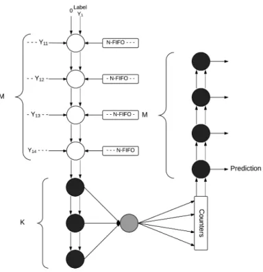
In a dependency graph an algorithm is decomposed in a set of composable atomic operations. The different colored circles (PE - Processing Elements) represent the different kinds of atomic operations. Each PE computes a partial result as a function of the incoming data from upstream PEs.

Figure4.1shows the data dependency graph of the K-Nearest Neighbor classifier. Yxy corre-sponds to the y feature of the x Testing vector and Xxy to the y feature of the x Training vector. The white PEs compute an one-dimensional Manhattan distance which is added to the incoming partial distance of the upstream white PEs. The dark-grey PEs receive two distance-label pairs; the pair with the lowest distance is outputted in the horizontal direction and the other in the vertical direction. Finally, the light-grey PEs receive the label of one of the nearest neighbors, increment

(42)

20 Hardware Implementation

Figure 4.1: KNN Dependency Graph.

Given the invariant structure of the dependency graph, it provides a robust framework to de-sign scalable architectures — computing the K-Nearest Neighbors with one more training vector corresponds to an additional column of white and dark-grey PEs; one more dimension in the fea-ture space corresponds to an additional row of white PEs; one more nearest neighbor corresponds to one more row of dark-grey and light-grey PEs.

The dependency graph provides a useful visualization of the data dependencies of the algo-rithm and its core operations. The next step is to project a dependency graph to obtain a data flow graph with linear time execution and resource usage.

Figure4.2shows a modified signal flow graph obtained from the horizontal projection of the dependency graph, in which M is the dimension of the feature space, K the number of Nearest Neighbors and N the number of training vectors. This projection trades the ability to pipeline the computation of different testing vectors for a much lower resource usage. In fact the architecture of the dependency graph outputs a new result each cycle after a delay of M + K + N, while the architecture of Figure4.2outputs a new result every N cycles after M + K + N + M cycles. The additional M cycles of delay comes from the fact an additional pipeline of M dark-grey PEs were added to sort the counters, unlike the dependency graph which only outputs label with the high-est count. The following sections will detail the main decisions when implementing the DKNN algorithm.

4.1.1 Ideal Resolution Classification

If, after the diagnosis, only one sub-circuit reports potential faults, the DKNN classifier is skipped and the sub-circuit in question is reported as faulty. To identify this so called Ideal Resolution Classification, each dimension of the testing vector is sequentially checked for zero. A counter

(43)

4.1 DKNN Hardware Architecture 21

Figure 4.2: DKNN Signal Flow Graph.

keeps track of the number of zero dimensions and a register keeps the index of the last non-zero dimension. After M cycles the vector analysis is completed. If the counter is equal to one, the contents of the register hold the index of the only non-zero dimension which incidentally are the identifier of the predicted faulty sub-circuit. When the counter is higher than one, the DKNN is started.

In case the Ideal Resolution Classification is wrong, there is no way of providing further valid predictions and thus the system can not learn the true label of the testing vector and update the training data.

4.1.2 Distance Calculation

The DKNN classification starts with the distance calculation. To reduce the hardware complexity, it was chosen to compute the Manhattan instead of the standard Euclidean with no clear impact on system accuracy (1 %). Each white PE calculates the distance between one dimension of the testing vector and the same dimension of the incoming training vector, which is added to the incoming partial distance of the previous PE. The first white PE receives a partial distance of 0 like Figure4.2shows.

(44)

In the first iteration, the first PE calculates the partial distance of the first dimension of the testing vector to the first dimension of the training vector. All the other PEs are stalled since their incoming partial distances are not valid yet. In the second iteration the first PE calculates the distance between the first dimension of the testing vector to the first dimension of the second training vector. The second PE already has a valid partial distance coming from the previous iteration occurred in the first PE, so it calculates the distance between the second dimension of the testing vector to the second dimension of the first training vector. Generalizing the process, after all the PEs start computing, M different features of M consecutive training vectors will be fed into the PEs. Even though the memory subsystem retrieves one training vector per cycle there is a need to keep a FIFO buffer with the last M training vectors, since the PEs retrieve features from the last M training vectors.

Per requirement of the DKNN devised by [3], when a training vector has a label identifier which correspond to the index of a dimension which is zero in the testing vector, that training vector can not be used to compute the nearest neighbors. As the memory sub-system only outputs one vector per cycle, if one training vector is not fit for evaluation, the pipeline has to be stalled. So when the pipeline is staled, all PEs of all colors do not execute their functions and keep outputs of the previous execution. In fact the only element of the system that changes is the pointer of the next memory position which is incremented. Overall one cycle is wasted without any useful computation, but at least energy is saved since all PEs remain static.

All inputs are represented with suitable number of bits. To represent the intermediate partial distances between the PEs, the worst case is considered which is all the testing features being the highest representable number and the training features being the highest representable number of opposite sign. The final distance is then two times M times the maximum dimension, which correspond to a total of the number of bits of the input plus log base 2 of M plus 1.

4.1.3 Distance Sorting

After the distance calculation, the first dark-grey PE, below the white PE pipeline, receives the distance, label and also the index of the training vector to which they belong.

The dark-grey PE is initialized with the highest representable distance and compares the in-coming distance with the saved distance. If the inin-coming distance is smaller than the saved dis-tance, the saved distance is outputted to the next PE and the incoming distance is set as the new saved distance. Otherwise the saved distance is kept and the incoming distance goes directly to the next PE. Every time a distance is moved the corresponding label and index are moved with it. The saved labels and indexes are also an input that can be read by the the light-grey PE.

After all distances are feed into the dark-grey PEs, each PE will hold the distance, label and index of the K nearest training vectors to the testing vector being evaluated. The distances are kept in ascending order.

(45)

4.1 DKNN Hardware Architecture 23

4.1.4 Label Counting

A single grey PE reports the number of neighbors each label has. In each iteration the light-grey PE reads the saved label of consecutive dark-light-grey PEs and increments the label corresponding to that label. After K iterations the counter vector holds the number of hits each label has.

4.1.5 Label Sorting

There is another set of dark-grey PEs, after the counters vector, which sort the labels by their counts, instead of sorting distances like the previous dark-grey PEs. Algorithm1 shows sorting mechanism of the labels. The label sorting starts with the counters vector being iterated as input to the first dark-grey PE. The PE is initialized with the saved counter content as zero and the label as invalid. The incoming counter value is compared with the saved counter. If the incoming counter value is higher than the saved one, the saved counters passes to the next PE. If the saved label is invalid, the incoming counter is always saved. If the incoming counter is smaller than the saved one, the incoming counter goes to the next PE. If the counters have the same value, there is a need of a more complex untie mechanism unlike the distance sorting PE that treated higher and equal as the same case.

In every iteration the dark-grey PE compares the incoming and saved labels with each label of the nearest neighbors. An array of K bits is kept for the incoming and saved label. Each bit is set to one if the label is the same of the label of the neighbor, zero otherwise. The most significant bit of the array belongs to the comparison with the nearest neighbor. When there is a tie, the two arrays are compared as unsigned integers. The array with the closest neighbors with the same label as the counter being evaluated, has the highest number. So, if the incoming counter holds a neighbor nearer than that in the saved counter, the incoming counter is updated with the new saved counter, otherwise it goes for the next PE. As in the case of the distance ordering, when a counter moves the associated label moves with it.

After M iterations the saved labels of the PEs hold the ordered list of labels. Those labels are predictions with decreasing levels of confidence for the faulty sub-circuit.

4.1.6 Data Replacement

After one prediction, the diagnosis system fixes/replaces the predicted faulty sub-circuit and retests the core. Unlike the first test where all the potential faults grouped to the belonging sub-circuit, this test just needs to provide a binary result. If the system still shows a faulty behavior, the classifier predicts the next probable faulty sub-circuit. The classifier will iterate over the predictions until the faulty sub-circuit is found.

(46)

Data: Counters[M]; NearestLabels[K]; for i = 1 to M do

for j = 0 to i do

if Counters[i].counter > Counters[k].counter then temporary = Counters[i];

Counters[i] = Counters[j]; Counters[j] = temporary;

else if Counters[i].counter == Counters[k].counter then for l = 0 to K do

if NearestLabels[l] == Counters[i].label then temporary = Counters[i];

Counters[i] = Counters[j]; Counters[j] = temporary; break;

else if NearestLabels[l] == Counters[i].label then break; end else Counters[i]; end end end

Algorithm 1: Pseudo code of the label sorting algorithm.

vector and the true label, which is no more than the identifier of the real faulty circuit. The index allows to find and replace the training vector in main memory.

4.2 FPGA Implementation

The end goal of this work is to create a diagnosis system suitable to be integrated on chip as a learning system, able to identify stressed sub-circuits and allow for minimizing performance degradation. The process to achieve a performing system involves many iterative design steps and tweaking in face of the performance characterization results. It is not affordable to implement each version of the system in custom silicon as the cost would be not affordable. Instead, resorting to simulation and an intermediate prototyping platform are validation approaches commonly used in the preliminary phases of a system development process. Likewise, this approach was followed to design and test the diagnosis system being proposed here.

An FPGA (Field-Programmable Gate Array) provides a middle ground between purely be-havioral simulation and a custom silicon implementation. A typical FPGA has N-input Look Up Tables (N-LUTs) which can be loaded with the truth table of any N-input combinational function; it also has memory elements in the form of FFs (Flip-Flops) used to create sequential circuits. These two blocks can be combined to create different logic circuits, being the complexity of the logical function limited by the FPGA resources. Nevertheless, this flexibility comes at the cost of performance.

(47)

4.2 FPGA Implementation 25

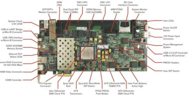
Figure 4.3: The Xilinx Zynq-7000 ZC706 Evaluation Kit.

A custom circuit allows for better resource usage than a circuit with one-size-fits-all kind of logic gates. There is also the issue of the in-chip network in the FPGA. For large logic systems, regardless the effectiveness of the routing algorithm, some signals will end up traveling half the FPGA chip to reach their destination. That is not the case with custom in chip networks with which this issue can be better dealt with. Since flexibility comes always at the cost of performance, FPGA designers decided to trade some flexibility and embed frequently used fixed function elements in the chip. Those elements include RAM blocks, multipliers, rocketIO, and even general purpose processors.

In the present case an FPGA was used to implement the DKNN classifier. The resources usage and execution speed in the FPGA can guide the optimization of the classifier for a future implementation of a high performance and low resource classifier in custom silicon. The Xil-inx Zynq-7000 ZC706 Evaluation Kit [34] was used. Next section provides some details of the platform and some functional considerations will be made.

4.2.1 Xilinx Zynq-7000 ZC706 Evaluation Kit

The ZC706 is a high-end board that comes with a large variety of communication options, among them: gigabit ethernet, PCI express, USB, HDMI, expansion connectors; it has 2 gigabytes of DDR3 memory, one gigabyte of them accessible by the programmable logic.

The FPGA chip is a System-on-Chip (SoC), the Zynq-7000 All Programmable SoC Z-7045. The SoC is composed of a Dual Core Cortex-A9 ARM [35] processor and the programmable logic

(48)

Figure 4.4: Communication system block diagram.

to accelerate any kind of computation. In this work instead of implementing the classifier and then communicate with it from the general purpose IO, the classifier will run as a co-processor of the main ARM processor.

Xilinx contributes to Linux Kernel and introduced support for the Zynq-7000 SoC. It even provides the binaries [36] of the kernel and bootloader to allow developers to run Linux distribu-tions on the ZC706 board. In this work, the Zynq’s SD Card was loaded with the Xilinx provided Kernel and the Arch Linux ARM operating system. The Zynq SoC Boot Mode DIP Switch (fig-ure 4.3) was set to allow booting from the SD Card. With the operating system running, SSH communication was set up to control the Zynq board from a computer in the network.

The Programmable Logic is configurable via a JTAG bus. The Zynq-7000 SoC has two JTAG ports, one accessible by the USB port present on the Board, and the other present in the ARM processor. To configure the Programmable Logic from the first JTAG port, one has to use the Vivado Design Suite and the whole board needs to be reset. The second port is mapped to the operating system running on the ARM processor as a char device. The Programmable Logic is configured while the operating system is running, without the need to reset the whole board.

4.2.2 Communication Interface

Up to know, there is an ARM processor running Linux and a classifier implemented in Verilog HDL ready to be synthesized for the FPGA. In this section, the communication system between the processor and the classifier will be detailed. Throughout this work the Vivado Design Suite was used to synthesize the classifier and the communication interface to the FPGA.

Vivado ships with the Intellectual Property (IP) core of the AMBA AXI protocol designed by ARM. AMBA AXI is an on-chip interconnection specification used to connect functional units inside a SoC. This protocol was used to connect the processor and the classifier.

Figure4.4shows the architecture of the implemented communication system. The rightmost block is the DKNN classifier, which was packaged on Vivado as an AXI slave core. The interface