www.atmos-meas-tech.net/3/209/2010/
© Author(s) 2010. This work is distributed under the Creative Commons Attribution 3.0 License.
Measurement
Techniques
A method for improved SCIAMACHY CO
2
retrieval in the presence
of optically thin clouds
M. Reuter, M. Buchwitz, O. Schneising, J. Heymann, H. Bovensmann, and J. P. Burrows
University of Bremen, Institute of Environmental Physics, P.O. Box 330440, 28334 Bremen, Germany
Received: 28 August 2009 – Published in Atmos. Meas. Tech. Discuss.: 8 October 2009 Revised: 15 January 2010 – Accepted: 9 February 2010 – Published: 12 February 2010
Abstract. An optimal estimation based retrieval scheme for satellite based retrievals of XCO2(the dry air column
aver-aged mixing ratio of atmospheric CO2) is presented enabling
accurate retrievals also in the presence of thin clouds. The proposed method is designed to analyze near-infrared nadir measurements of the SCIAMACHY instrument in the CO2
absorption band at 1580 nm and in the O2-A absorption band
at around 760 nm. The algorithm accounts for scattering in an optically thin cirrus cloud layer and at aerosols of a default profile. The scattering information is mainly obtained from the O2-A band and a merged fit windows approach enables
the transfer of information between the O2-A and the CO2
band. Via the optimal estimation technique, the algorithm is able to account for a priori information to further constrain the inversion. Test scenarios of simulated SCIAMACHY sun-normalized radiance measurements are analyzed in order to specify the quality of the proposed method. In contrast to existing algorithms for SCIAMACHY retrievals, the system-atic errors due to cirrus clouds with optical thicknesses up to 1.0 are reduced to values below 4 ppm for most of the ana-lyzed scenarios. This shows that the proposed method has the potential to reduce uncertainties of SCIAMACHY retrieved XCO2making this data product potentially useful for surface
flux inverse modeling.
1 Introduction
CO2is the dominant anthropogenic greenhouse gas but there
are still large uncertainties of its natural global sources and sinks (Stephens et al., 2007). Global measurements of the atmospheric CO2 concentration can be used as input
Correspondence to:M. Reuter
for inverse models to reduce these uncertainties. In-situ CO2 measurements of networks such as the NOAA
(Na-tional Oceanic and Atmospheric Administration) carbon cy-cle greenhouse gas cooperative air sampling network (http: //www.esrl.noaa.gov/gmd/ccgg/flask.html) are very accurate. However, the sparseness of the measurement sites and their world wide distribution with a majority over US and Euro-pean land surfaces and a minority on the Southern Hemi-sphere limit the current knowledge of CO2 surface fluxes.
Theoretical studies have shown that satellite measurements of CO2have the potential to significantly reduce the surface
flux uncertainties. This requires a precision of about 1% for regional averages and monthly means (Rayner and O’Brien, 2001; Houweling et al., 2004). However, undetected biases of a few tenths of a part per million on regional scales can already hamper inverse surface flux modeling (Miller et al., 2007; Chevallier et al., 2007).
Currently, there are only a few satellite instruments in orbit which are able to measure atmospheric CO2. The High
Res-olution Infrared Radiation Sounder (HIRS) (Ch´edin et al., 2002, 2003), the Atmospheric InfraRed Sounder (AIRS) (En-gelen et al., 2004; En(En-gelen and McNally, 2005; Aumann et al., 2005; Strow et al., 2006; Maddy et al., 2008), and the Infrared Atmospheric Sounding Interferometer (IASI) (Crevoisier et al., 2009) perform CO2 sensitive
measure-ments in the thermal infrared (TIR) spectral region, i.e. these instruments do not detect reflected solar radiation but ther-mal radiation emitted from surface and atmosphere. This brings the advantage that measurements are possible not only at day-time but also at night-time. However, the disadvantage of such measurements is their lack of sensitivity in the lower troposphere where the strongest signals due to sources and sinks can be expected.
(with height) and shows maximum values near the surface, typically. Note that in this paper NIR and SWIR are com-monly referred to as NIR. At present, SCIAMACHY aboard ENVISAT launched in 2002 (Bovensmann et al., 1999) and TANSO (Thermal And Near infrared Sensor for carbon Observation) aboard GOSAT (Greenhouse gases Observing SATellite) launched in 2009 (Yokota et al., 2004) are the only orbiting instruments measuring NIR radiation in appropriate absorption bands at around 0.76, 1.6, and 2.0 µm with suf-ficient spectral resolution to retrieve XCO2. Another
car-bon dioxide observing satellite was OCO (Orbiting Carcar-bon Observatory) (Crisp et al., 2004). OCO was designed to measure within the same spectral region. Unfortunately, the satellite was lost shortly after lift-off on 24 February 2009 (Palmer and Rayner, 2009).
Contrary to TANSO, SCIAMACHY was not especially designed for the retrieval of XCO2with the precision and
ac-curacy needed to enhance our knowledge about sources and sinks via inverse modeling. Due to SCIAMACHY’s lower spatial and spectral resolution, the achievable accuracy and precision is expected to be lower compared to a TANSO like instrument. Nevertheless, within the time period 2002–2009 SCIAMACHY was the only instrument measuring XCO2
from space with significant sensitivity also to the lower tro-posphere. Therefore, the development of algorithms deriving XCO2from SCIAMACHY as accurate as possible with
real-istic error estimates is crucial to start a consistent long-term time series of XCO2observations from space.
In the literature one can find several somewhat differ-ent XCO2retrieval algorithms for SCIAMACHY data: The
WFM-DOAS algorithm (Weighting Function Modified Dif-ferential Optical Absorption Spectroscopy) was developed at the University of Bremen for the retrieval of trace gases from SCIAMACHY and has been described by Schneising et al. (2008), Buchwitz et al. (2005a,b, 2000b), and Buchwitz and Burrows (2004). This algorithm is based on a fast look-up table (LUT) based forward model used to derive the num-ber of CO2and O2molecules in the atmospheric column in
order to derive XCO2. Other groups have developed
some-what different approaches to retrieve XCO2or CO2columns
from SCIAMACHY. The computationally much more ex-pensive FSI/WFM-DOAS algorithm (Full Spectral Initiation WFM-DOAS) described by (Barkley et al., 2006a,c,b, 2007) derives XCO2 by retrieving the number of CO2 molecules
from SCIAMACHY but determining the air column from meteorological analysis of the surface pressure. This ap-plies also to the algorithm discussed by Houweling et al. (2005). The retrieval algorithm designed for OCO follows the strategy to determine XCO2from column measurements
of CO2and simultaneous measurements of the surface
pres-sure derived from meapres-surements in the O2-A band (Connor
et al., 2008). B¨osch et al. (2006) applied a modified ver-sion of this algorithm with a reduced number of state vec-tor elements to SCIAMACHY data in a surrounding of the Park Falls FTS-site. As SCIAMACHY’s channel 7 suffers
from a light-leak and ice on the detector, all these algorithms derive the number of CO2 molecules from the weak CO2
absorption band at around 1.6 µm and not from the much stronger band at around 2.0 µm. B¨osch et al. (2006) and Schneising et al. (2008) showed that XCO2can be retrieved
from SCIAMACHY with a single measurement precision of 1–2% assuming clear sky conditions. Additionally, Schneis-ing et al. (2008) showed that a relative accuracy of about 1–2% for monthly averages at a spatial resolution of about 7◦×7◦ can be achieved from SCIAMACHY measurements under clear sky conditions.
However, scattering at aerosol and/or cloud particles re-mains a major source of uncertainty for SCIAMACHY XCO2retrievals which easily exceeds the precisions and
ac-curacy estimated for clear sky conditions. Houweling et al. (2005) found that the XCO2 retrieval error may amount to
10% in the presence of mineral dust aerosols. Schneising et al. (2008) showed that a thin scattering layer with an opti-cal thickness of 0.03 in the upper troposphere can introduce XCO2 uncertainties of up to several percent. They derived
a XCO2error of 8.80% resulting from a CO2column error
of−0.89% and a O2column error of−8.91% for a scenario
with an albedo of 0.1. Aben et al. (2007) found an underesti-mation of space-based measurements of the CO2column of
8% for a scenario with a cirrus cloud optical thickness (COT) of 0.05 and a surface albedo of 0.05. The underestimation amounted to 1% for an albedo of 0.5.
Unfortunately, thin clouds with optical thicknesses below 0.1 cannot easily be detected within nadir measurements in the visible and near infrared spectral region (e.g. Reuter et al., 2009; Rodriguez et al., 2007).
Satellite occultation measurements as well as lidar obser-vations show that sub visible cirrus clouds occur quite fre-quently with a maximum occurrence probability of about 45% within the tropics, seasonally following the inter tropi-cal convergence zone (ITCZ) (Wang et al., 1996; Winker and Trepte, 1998; Nazaryan et al., 2008). The WFM-DOAS 1.0 XCO2 retrieval for SCIAMACHY has a low quality over
dark ocean surfaces and is therefore applied to land surfaces only. The global distribution of the continents shows that the land masses of the Southern Hemisphere are closer to the equator. For this reason, southern hemispheric SCIA-MACHY XCO2 retrievals are statistically much more
af-fected by undetected sub visible cirrus clouds compared to northern hemispheric retrievals. Analyzing data of the li-dar instrument CALIOP (Cloud-Aerosol LIli-dar with Orthog-onal Polarization) aboard the CALIPSO satellite (Cloud-Aerosol Lidar and Infrared Pathfinder Satellite Observa-tions), Schneising et al. (2008) found that discrepancies of the southern hemispheric annual cycle of SCIAMACHY re-trieved XCO2and corresponding values of NOAA’s CO2
Having in focus the spectrally high resolving satellite in-struments TANSO aboard GOSAT and OCO, algorithms have been developed to correct for scattering effects. Bril et al. (2007) developed a method which is based on appli-cation of the equivalence theorem and photon path-length statistics with further parameterization of the photon path-length probability density function (PPDF) for a TANSO like instrument. They derive effective scattering parameters of cirrus clouds and aerosols from the O2-A band and from
sat-urated water vapor lines at around 2.0 µm. This information is used to correct the CO2retrieval in the 1.6 µm CO2band.
Kuang et al. (2002) proposed a method based on simultane-ously fitting cloud and aerosol parameters (and others) within the three spectral bands of OCO at around 0.76, 1.6, and 2.0 µm. They estimated that a precision of 0.3 to 2.5 ppm is achievable for aerosol optical thicknesses (AOT) of up to 0.3. In contrast to both methods, the XCO2retrieval algorithms
for SCIAMACHY mentioned above do not explicitly ac-count for scattering effects. They either do not acac-count for scattering at all or in an indirect way as the WFM-DOAS al-gorithm does by assuming that photon path-length modifica-tions are identical at 0.76 and 1.6 µm. In this approximation, scattering errors of CO2and O2cancel out when calculating
XCO2.
Within the publication at hand, a new XCO2retrieval
algo-rithm optimized for SCIAMACHY nadir data is introduced explicitly considering scattering in an (optically thin) ice cloud layer and at aerosols of a default profile. The physical basis for simultaneously retrieving scattering related param-eters and XCO2using a merged fit windows approach is
de-scribed in Sect. 2. The information about these scattering pa-rameters comes mainly from the measurements in the O2fit
window. The usability of SCIAMACHY or GOME measure-ments in this spectral region for the retrieval of cloud param-eters is already confirmed within several publications (e.g. Kokhanovsky et al., 2006; Wang et al., 2008; van Dieden-hoven et al., 2007). Section 3 describes the inversion tech-nique based on optimal estimation. Within this section, de-tails of the forward operator, the state vector, and the usage of prior knowledge is discussed. An error analysis is given in Sect. 4. Here, the retrieval algorithm is applied to simu-lated SCIAMACHY data in order to specify the algorithm’s sensitivity to the state vector elements but also to parameters that are not retrieved within the state vector. In this regard, special emphasis is put on cloud parameters which are not retrieved.
2 Physical basis
The WFM-DOAS algorithm (Schneising et al., 2008; Buch-witz et al., 2005a,b, 2000b; BuchBuch-witz and Burrows, 2004) re-trieves several independent parameters from SCIAMACHY measurements in the spectral region dominated by CO2
absorption from 1558 to 1594 nm (in the following referred
to as the “CO2fit window”) and also from measurements in
the spectral region of the O2-A band from 755 to 775 nm (in
the following referred to as the “O2fit window”). Within the
CO2fit window the number of CO2molecules, the number of
H2O molecules, the atmospheric temperature, spectral shift
and squeeze, and a 2nd order polynomial are retrieved. The number of CO2molecules is retrieved by shifting a reference
profile with constant mixing ratio. In the same manner, the number of H2O molecules as well as the atmospheric
tem-perature is determined by shifting reference profiles. Sep-arately from this, the number of O2 molecules, the
atmo-spheric temperature, spectral shift and squeeze, and a 2nd order polynomial are retrieved in an analogous way from the O2fit window. Beforehand, an albedo retrieval is performed
in both fit windows using measurements in micro windows (nearly) without absorptions line features at the edge of both fit windows.
Each of these parameters influences the spectrum of re-flected solar radiation measured at the satellite instrument. The partial derivatives of the measured radiation with respect to a parameter is called the weighting function (or Jacobian) of this parameter. Of course, it is only possible to retrieve those parameters having a unique weighting function, suffi-ciently different from all other weighting functions in terms of the instrument’s precision. Very similar weighting func-tions can result in ambiguities of the retrieved corresponding parameters.
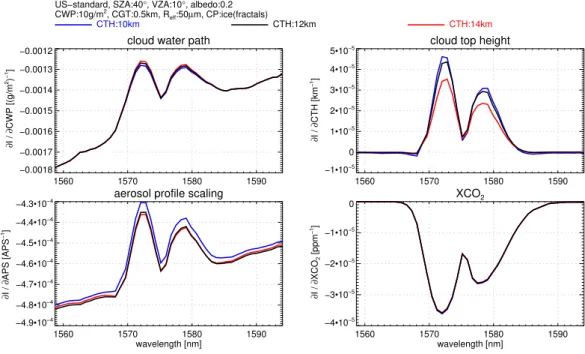
Figure 1 shows for exemplary atmospheric conditions with moderate aerosol load and one thin ice cloud layer the weighting functions of three different scattering re-lated parameters under a typical observation geometry in SCIAMACHY’s spectral resolution. Additionally, the figure shows the XCO2weighting function which gives the change
of radiation when columnar increasing the CO2
concentra-tion by 1 ppm. For this example, the magnitude of its spectral signature is comparable to a change of the cloud top height (CTH) by 1 km, the cloud water/ice path (CWP) by 0.2 g/m2, or to a change of the aerosol load by 100%. It is immedi-ately noticeable that there are high correlations between the curves. Especially between the aerosol profile scaling (APS) and the cloud water/ice path weighting function as well as be-tween the cloud top height and the XCO2weighting function.
XCO2 changes of 1 ppm are approximately the detection
limit due to SCIAMACHY’s signal to noise (SNR) charac-teristics. This means, with SCIAMACHY it is actually not possible to discriminate XCO2 values of a few ppm from
changes of the given scattering parameters. For example, de-creasing the cloud top height from 14 to 10 km spectrally changes the radiation in (nearly) the same way as increas-ing XCO2 by 4 ppm does. Most likely, it is not possible to
retrieve scattering parameters simultaneously with the num-ber of CO2molecules, i.e. uncertainties of the scattering
pa-rameters will always result in uncertainties of the retrieved CO2 molecules when solely analyzing measurements from
cloud top height
1560 1570 1580 1590
−1•10−5
0
1•10−5
2•10−5
3•10−5
4•10−5
5•10−5
∂
I /
∂
CTH [km
−1]
cloud water path
1560 1570 1580 1590
−0.0018 −0.0017 −0.0016 −0.0015 −0.0014 −0.0013 −0.0012
∂
I /
∂
CWP [(g/m
2) −1]
XCO2
1560 1570 1580 1590
wavelength [nm]
−4•10−5
−3•10−5
−2•10−5
−1•10−5
0
∂
I /
∂
XCO
2
[ppm
−1]
aerosol profile scaling
1560 1570 1580 1590
wavelength [nm]
−4.9•10−4
−4.8•10−4
−4.7•10−4
−4.6•10−4
−4.5•10−4
−4.4•10−4
−4.3•10−4
∂
I /
∂
APS [APS
−1]
US−standard, SZA:40°, VZA:10°, albedo:0.2
CWP:10g/m2, CGT:0.5km, R
eff:50µm, CP:ice(fractals)
CTH:10km CTH:12km CTH:14km
Fig. 1. Weighting functions in the CO2fit window for three cloud scenarios based on a US-standard atmosphere including an optically thin
ice cloud with a cloud top height of 10 km (blue), 12 km (black), and 14 km (red): cloud water/ice path (top/left), cloud top height (top/right), scaling of the aerosol profile (bottom/left), and XCO2 (bottom/right). The weighting functions are calculated with the SCIATRAN 3.0 radiative transfer code and are folded with SCIAMACHY’s slit function.
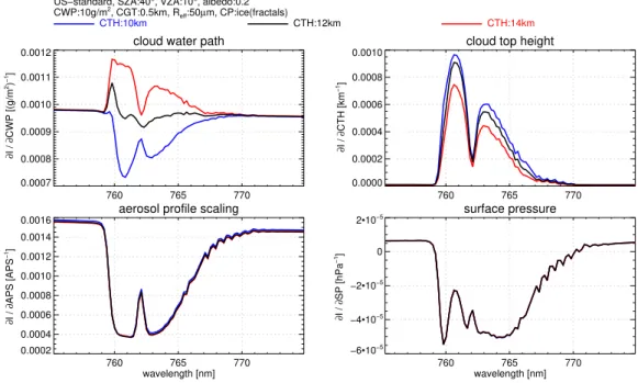
Analogous to Fig. 1, Fig. 2 shows for identical atmo-spheric conditions the weighting functions of the same scat-tering parameters but for the O2 fit window. Additionally,
it shows the weighting function in respect to surface pres-sureps which can be used to derive the total number of air
molecules within the atmospheric column by applying the hydrostatic assumption. The similarities between the weight-ing functions are less pronounced in this fit window. This ap-plies especially when comparing the surface pressure weight-ing function to the weightweight-ing functions of the given scatter-ing parameters. This originates by much stronger tion lines in this fit window. As width and depth of absorp-tion lines depend on the ambient pressure, saturaabsorp-tion effects differ much stronger with height within this spectral region. Additionally, SCIAMACHY’s resolution resolves the spec-tral structures of the gaseous absorption better within this fit window. Nevertheless, there are still similarities that are not negligible e.g. between the cloud top height and aerosol pro-file scaling weighting function. Differences of 1 hPa are in the order of the detection limit according to SCIAMACHY’s SNR characteristics. Therefore, it can be expected that inde-pendent information on the given scattering parameters can be extracted from this fit window simultaneously with infor-mation about the surface pressure.
The large differences of the three illustrated cloud top height weighting functions show that the radiative transfer can become non-linear in respect to this parameter. Addi-tionally, the spectral similarity of the CTH and the CWP
weighting function strongly depend on the scenario (large differences for the cloud at 12 km, minor differences for the cloud at 10 km). This means, depending on the individual scene, ambiguities may be more or less pronounced. In this context, also the selected surface albedo has strong influence. In the following section we will describe, how the infor-mation on scattering parameters, which can be derived from the O2fit window, can be transported to the CO2fit window.
3 Inversion via optimal estimation
We use an optimal estimation based inversion technique to find the most probable atmospheric state given a SCIA-MACHY measurement and some prior knowledge. Nearly all mathematical expressions given in this publication as well as their derivation and notation can be found in the text book of Rodgers (2000). A list of all used symbols is given by Table 1.
The forward modelF is a vector function which calcu-lates for a given (atmospheric) state simulated measurements i.e. simulated SCIAMACHY spectra. The input for the for-ward model are the state vectorxand the parameter vectorb. The state vector consists of all unknown variables that shall be retrieved from the measurement (e.g. CO2). Parameters
cloud top height
760 765 770
0.0000 0.0002 0.0004 0.0006 0.0008 0.0010
∂
I /
∂
CTH [km
−1]
cloud water path
760 765 770
0.0007 0.0008 0.0009 0.0010 0.0011 0.0012
∂
I /
∂
CWP [(g/m
2) −1]
surface pressure
760 765 770
wavelength [nm]
−6•10−5
−4•10−5
−2•10−5
0
2•10−5
∂
I /
∂
SP [hPa
−1]
aerosol profile scaling
760 765 770
wavelength [nm] 0.0002
0.0004 0.0006 0.0008 0.0010 0.0012 0.0014 0.0016
∂
I /
∂
APS [APS
−1]
US−standard, SZA:40°, VZA:10°, albedo:0.2
CWP:10g/m2, CGT:0.5km, R
eff:50µm, CP:ice(fractals)
CTH:10km CTH:12km CTH:14km
Fig. 2. Weighting functions in the O2fit window for three cloud scenarios based on a US-standard atmosphere including an optically
thin ice cloud with a cloud top height of 10 km (blue), 12 km (black), and 14 km (red): cloud water/ice path (top/left), cloud top height (top/right), scaling of the aerosol profile (bottom/left), and surface pressure (bottom/right). The weighting functions are calculated with the SCIATRAN 3.0 radiative transfer code and are folded with SCIAMACHY’s slit function.
is given in the first column of Table 3. The measurement vec-toryconsists of SCIAMACHY sun-normalized radiances of two merged fit windows concatenating the measurements in the CO2and O2fit window. The difference of measurement
and corresponding simulation by the forward model is given by the error vectorεcomprising inaccuracies of the instru-ment and of the forward model:
y=F(x,b)+ε (1)
According to Eq. (5.3) of Rodgers (2000), we aim to find the state vectorxwhich minimizes the cost functionχ2: χ2=(y−F(x,b))TS−ǫ1(y−F(x,b))
+(x−xa)TSa−1(x−xa) (2)
Here,Sǫ is the error covariance matrix corresponding to the
measurement vector, xa is the a priori state vector which
holds the prior knowledge about the state vector elements andSais the corresponding a priori error covariance matrix
which specifies the uncertainties of the a priori state vector elements as well as their cross correlations.
Even though the number of state vector elements (26) is smaller than the number of measurement vector elements (134), the inversion problem is generally under-determined. The weighting functions of some state vector elements show quite large correlations under certain conditions. This es-pecially applies to the weighting functions corresponding to
the ten-layered CO2profile but also to some of the
weight-ing functions shown in Figs. 1 and 2. For this reason we use a priori knowledge further constraining the problem and making it well-posed. However, for most of the state vector elements the used a priori knowledge gives only a weak con-straint and is therefore not dominating the retrieval results. Furthermore, we use only static (i.e. spatially and temporally invariant) a priori knowledge of XCO2.
According to Eq. (5.8) of Rodgers (2000), we use a Gauss-Newton method to iteratively find the state vectorxˆ which minimizes the cost function.
xi+1=xi+ ˆS[KTi S
−1
ǫ (y−F(xi,b))−S−a1(xi−xa)] (3)
ˆ
S=(KTi Sǫ−1Ki+S−a1)
−1 (4)
Within this equation, Kis the Jacobian or weighting func-tion matrix consisting of the derivatives of the forward model in respect to the state vector elementsK=∂F(x,b))/∂x. In the case of convergence,xi+1is the most probable solution
given the measurement and the prior knowledge and is then denoted as maximum a posteriori solutionxˆ of the inverse problem. Sˆ is the corresponding covariance matrix consist-ing of the variances of the retried state vector elements and their correlations.
The iteration starts with the first guess state vector x0.
Often, x0 is set toxa, even though this is mathematically
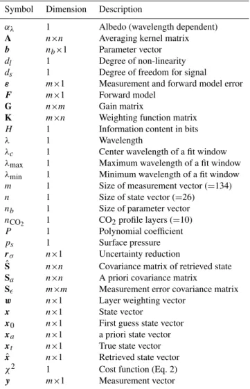
Table 1. List of used symbols and corresponding dimensions and short descriptions.
Symbol Dimension Description
αλ 1 Albedo (wavelength dependent)
A n×n Averaging kernel matrix
b nb×1 Parameter vector
dl 1 Degree of non-linearity
ds 1 Degree of freedom for signal
ε m×1 Measurement and forward model error
F m×1 Forward model
G n×m Gain matrix
K m×n Weighting function matrix
H 1 Information content in bits
λ 1 Wavelength
λc 1 Center wavelength of a fit window
λmax 1 Maximum wavelength of a fit window
λmin 1 Minimum wavelength of a fit window
m 1 Size of measurement vector (=134)
n 1 Size of state vector (=26)
nb 1 Size of parameter vector
nCO2 1 CO2profile layers (=10)
P 1 Polynomial coefficient
ps 1 Surface pressure
rσ n×1 Uncertainty reduction
ˆ
S n×n Covariance matrix of retrieved state
Sa n×n A priori covariance matrix
Sǫ m×m Measurement error covariance matrix
w n×1 Layer weighting vector
x n×1 State vector
x0 n×1 First guess state vector
xa n×1 a priori state vector
xt n×1 True state vector
ˆ
x n×1 Retrieved state vector
χ2 1 Cost function (Eq. 2)
y m×1 Measurement vector
we test for convergence by relating the changes of the state vector to the error covarianceSˆ after each iteration. If the value of(xi−xi+1)TSˆ−1(xi−xi+1)falls below the number
of state vector elements (26), we assume that convergence is achieved and stop the iteration. As it is theoretically possible that convergence is never achieved, we stop the iteration after ten unsuccessful steps. However, typically, the convergence criterion is fulfilled after two to four iterations.
Subsequently, we use some terms also given by Rodgers (2000) to compute the gain matrixG(Eq. 2.45), the averag-ing kernel matrixA(Eq. 3.10), the degree of freedom for sig-nalds (Eq. 2.80), and the information contentH (Eq. 2.80).
The gain matrix corresponds to the sensitivity of the retrieval to the measurement and is given by:
G=(KTS−ǫ1K+S−a1)KTS−ǫ1 (5)
Having the gain matrix, we can compute the averaging kernel matrix which is the sensitivity of the retrieval to the true state:
A=GK (6)
The degree of freedom for signal corresponds to the number of independent quantities that can be derived from the mea-surement and is given by:
ds=tr(A) (7)
The information content gives the number of different atmo-spheric states that can be distinguished in bits:
H= −1
2ln(|I−A|) (8)
The degree of freedom as well as the information content can be calculated for arbitrary sub sets of state vector elements by taking only corresponding elements of the averaging ker-nel matrix into account. Comparing the variances of the re-trieved state vector elements with the corresponding a priori variances, the uncertainty reductionrσ of thejt hstate vector
element is defined by:
rσ j=1−
q ˆ
Sj,j/Sa j,j (9)
Note: Using merged fit windows instead of performing a CO2 and a O2 retrieval independently within two separate
fit windows has two main advantages when retrieving state vector elements which have sensitivities in both fit windows. 1) These elements are better constrained because simultane-ous fitting implicitly utilizes the knowledge that the retrieved quantity (e.g. the atmospheric temperature) must be identi-cal in both fit windows. 2) If there are state vector elements with strong ambiguities in one fit windows (e.g. surface pres-sure and scattering parameters in the CO2fit window), the
information come mainly from the fit window with less am-biguities. Merging the fit windows makes this information available in both fit windows.
3.1 Forward model
All radiative transfer calculations utilized for our studies are calculated with the SCIATRAN 3.0 radiative transfer code (Rozanov et al., 2005) in discrete ordinate mode. We use the correlated-k approach of Buchwitz et al. (2000a) to increase the computational efficiency. As final part of the forward calculation, the resulting spectra are folded with a SCIA-MACHY like Gaussian slit function and the dead/bad pixel mask also used for WFM-DOAS 1.0 is applied. Spectral line parameters are taken from the HITRAN 2008 (Rothman et al., 2009) database.
The radiative transfer calculations are performed on 60 model levels, even though our state vector includes only a ten-layered CO2 mixing ratio profile. This profile is
In the case of liquid water droplets, phase function, extinc-tion, and scattering coefficient of cloud particles are calcu-lated with Mie’s theory assuming gamma particle size distri-butions.
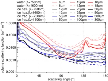
In the case of ice crystals, corresponding calculations are performed with a Monte Carlo code, assuming an ensemble of randomly aligned fractal or hexagonal particles. The vol-ume scattering function is the product of phase function and scattering coefficient. Figure 3 illustrates the volume scatter-ing functions of all cloud particles analyzed in Sect. 4.
3.2 State vector
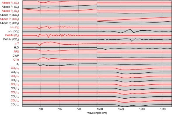
All retrieval results shown here are valid for a state vector consisting of 26 elements listed in the first column of Ta-ble 3. Corresponding weighting functions calculated for ex-emplary atmospheric conditions are illustrated in Fig. 4. This figure shows that not only the scattering parameter weighting functions may have cross correlations with other weightung functions. In this context, e.g. the albedo weighting functions show strong similarities to the scattering related weighting functions. For all state vector elements, we aim at obtaining realistic a priori uncertainties which sufficiently constrain the inversion by defining a well-posed problem without dominat-ing the retrieval results.
3.2.1 Wavelength shift, slit function FWHM
The state vector accounts for fitting a wavelength shift and the full width half maximum (FWHM) of a Gaussian shaped instrument’s slit function separately in the O2 and CO2 fit
window. This means, the corresponding weighting functions are identical zero within the O2or in the CO2 fit window,
respectively.
3.2.2 Albedo
We assume a Lambertian surface with an albedo α with smooth spectral progression which can be expressed by a 2nd order polynomial separately within both fit windows.
αλ=P0+P1
λ−λc
λmax−λmin
+P2(
λ−λc
λmax−λmin
)2 (10)
Here,P0,P1, andP2are the polynomial coefficients,λthe
wavelength, λc the center wavelength, λmin the minimum,
andλmaxthe maximum wavelength within the fit window. In
order to get good first guess and a priori estimates for the 0th polynomial coefficients, we use the look-up table based albedo retrieval described by Schneising et al. (2008). This estimates the albedo within a micro window not influenced by gaseous absorption lines at one edge of each fit window assuming a cloud free atmosphere with moderate aerosol load. We use an a priori uncertainty of 0.05 for the 0th poly-nomial coefficients. The first guess and the a priori values of the 1st and 2nd polynomial coefficients are zero. Their
0 45 90 135 180
scattering angle [°] 0.0001
0.0010 0.0100 0.1000 1.0000
volume scattering function [sr
−1
m
−1
]
water (λ=750nm) water (λ=1600nm) ice hex. (λ=750nm) ice hex.(λ=1600nm) ice frac. (λ=750nm) ice frac.(λ=1600nm)
6µm 6µm 12µm 12µm 50µm 50µm
12µm 12µm 25µm 25µm 100µm 100µm
18µm 18µm 50µm 50µm 300µm 300µm
Fig. 3. Volume scattering functions of all cloud particles analyzed
in Sect. 4. The dominant forward peaks is cut in this clipping.
estimated a priori uncertainties are 0.01 and 0.001, respec-tively. The magnitude of these values is typical for 2nd order polynomial coefficients fitted to the natural surfaces albedos shown in Fig. 5.
3.2.3 CO2mixing ratio profile
The CO2mixing ratio is fitted within 10 atmospheric layers,
splitting the atmosphere in equally spaced pressure intervals normalized by the surface pressureps (0.0,0.1,0.2,...,1.0).
We analyzed CarbonTracker data over land surfaces of the years 2003 to 2005 to determine a static a priori statistic for the CO2mixing ratio in corresponding pressure levels. The
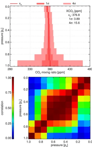
resulting a priori state vector elements, their standard devi-ation and correldevi-ation matrix are shown in Fig. 6. It is not surprising that the largest variability is observed in the low-est 10% of the atmosphere. From the correlation matrix it is also visible that there are large cross correlations in the boundary layer, the free troposphere, and the stratosphere.
As the shape of the CO2 weighting functions in
SCIA-MACHY resolution shows only minor changes with height, it cannot be expected that there is much information obtain-able about the CO2profile shape from SCIAMACHY nadir
measurements. Therefore, we use a relatively narrow con-straint for the profile shape but simultaneously a rather weak constraint for XCO2. For this reason, we build the CO2part
of the a priori covariance matrix by using the correlation ma-trix as is but using a four times increased standard deviation. As a result, the a priori uncertainty of XCO2increases from
3.9 to 15.6 ppm. The average XCO2of all analyzed
CO2 L0
CO2 L1
CO2 L2
CO2 L3
CO2 L4
CO2 L5
CO2 L6
CO2 L7
CO2 L8
CO2 L9
ps
CTH
CWP
APS
H2O
∆ T
FWHM (CO2)
FWHM (O2)
∆λ (CO
2)
∆λ (O 2)
Albedo P2 (CO2)
Albedo P1 (CO2)
Albedo P0 (CO2)
Albedo P2 (O2)
Albedo P1 (O2)
Albedo P0 (O2)
760 765 770 1560 1570 1580 1590
wavelength [nm]
Fig. 4. Weighting functions (scaled to the same amplitude) calculated with the SCIATRAN 3.0 radiative transfer code for the first guess
state vector of the “met. 1σ” scenario at 40◦solar zenith angle.
3.2.4 Atmospheric profiles
With regard to the application to real SCIAMACHY mea-surements, we plan to use atmospheric profiles of pressure, temperature, and humidity provided by ECMWF (European Center for Medium-range Weather Forecasts) for the forward model calculations as part of the parameter vector. Applying the hydrostatic assumption, the surface pressure determines the total number of air molecules within the atmospheric col-umn. Therefore, it is a critical parameter for the retrieval of XCO2.
We compared a dataset of more than 8000 radiosonde mea-surements of the year 2004 within−70◦E to 55◦E longitude and−35◦N to 80◦N latitude with corresponding ECMWF profiles. The exact SCIAMACHY sub pixel composition of surface elevations is not perfectly known. For this reason, we used unmodified ECMWF profiles i.e. we performed no interpolation of the surface height within the ECMWF pro-files. Therefore, the surface elevation within a radiosonde profile may differ from the surface elevation within the pro-file of the corresponding ECMWF grid box. This means, our estimate combines two uncertainties: The ECMWF sur-face pressure uncertainty and the sub grid box sursur-face pres-sure variability due to topography which is most times much larger. This is only a rough estimate that certainly drastically overestimates the true ECMWF surface pressure precision for cases where an interpolation to the true topography within
the instrument’s field of view can be applied. However, this overestimation ensures that we do not over constrain the re-trieval in respect to surface pressure.
Resulting from these comparisons, we estimated that the surface pressure is known with a standard deviation of 3.2%. The standard deviation of the temperature shift between mea-sured and modeled temperature profiles amounts to 1.1 K. The corresponding value for a scaling of the H2O profile is
32%. The biases were much smaller than the standard devia-tions. Therefore, we apply no bias to the a priori knowledge of surface pressure, temperature profile shift, and scaling of the humidity profile.
3.2.5 Scattering parameters
Scattering can cause very complex modifications of the satel-lite observed radiance spectra and there is nearly an infi-nite amount of micro and macro physical parameters that are needed to comprehensively account for all scattering effects in the forward model. However, as illustrated in Figs. 1 and 2 it is unlikely possible to retrieve many of these parameters simultaneously from SCIAMACHY measurements in the O2
fit window. The same applies to the CO2fit window which
700 900 1100 1300 1500 1700 wavelength [nm]
0.0 0.2 0.4 0.6 0.8 1.0
albedo
snow sand conifers
ocean soil
deciduous rangeland
Fig. 5. Spectral albedos of different natural surface types.
Repro-duced from the ASTER Spectral Library through the courtesy of the Jet Propulsion Laboratory, California Institute of Technology, Pasadena, California (©1999, California Institute of Technology) and the Digital Spectral Library 06 of the US Geological Survey.
spectral signatures which makes them distinguishable from other weighting functions. These parameters are cloud top height, cloud water/ice path whereas water/ice stands for ice and/or liquid water, and the aerosol scaling factor for a de-fault aerosol profile. All other scattering related parameters are not part of the state vector but only part of the parameter vector and are set to constant values.
Within the parameter vector we define that scattering at particles takes place in a plane parallel geometry at one cloud layer with a geometrical thickness of 0.5 km homo-geneously consisting of fractal ice crystals with 50 µm ef-fective radius. In addition, scattering happens at a stan-dard LOWTRAN summer aerosol profile with moderate ru-ral aerosol load and Henyey-Greenstein phase function and a total aerosol optical thickness of about 0.136 at 750 nm and 0.038 at 1550 nm. Both cloud parameters are aimed at opti-cally thin cirrus clouds because on the one hand it is not pos-sible to get enough information from below an optically thick cloud and on the other hand the foregoing cloud screening fil-ters already the optically thick clouds. Additionally, Schneis-ing et al. (2008) found that thin cirrus clouds are most likely the reason for shortcoming of the WFM-DOAS 1.0 CO2
re-trieval on the Southern Hemisphere.
We set the a priori value of CTH to 10 km with a one sigma uncertainty of 5 km. Both values are only rough estimates for typical thin cirrus clouds. Nevertheless, the size of the one sigma uncertainty seems to be large enough to avoid over-constraining the problem as it covers large parts of the upper troposphere where these clouds occur.
All micro physical cloud and aerosol parameters are as-sumed to be constant and known. This assumption is obvi-ously not true. Scattering strongly depends on the size of the scattering particles e.g. scattering is more effective at clouds
280 330 380 430 480
CO2 mixing ratio [ppm]
1.0 0.8 0.6 0.4 0.2 0.0
pressure [p
s
]
xa 1σ 4σ
XCO2 [ppm]
xa: 376.8
1σ: 3.89
4σ: 15.6
0.00 0.25 0.50 0.75 1.00
correlation
1.0 0.8 0.6 0.4 0.2 0.0
pressure [ps]
1.0 0.8 0.6 0.4 0.2 0.0
pressure [p
s
]
Fig. 6. Static a priori knowledge of the ten-layered CO2mixing
ra-tio profile calculated from three years (2003–2005) CarbonTracker data over land surfaces. Top: A priori state vector values and their 1σand 4σ uncertainties. Bottom: Correlation matrix.
with smaller particles. For this reason, it is not possible to derive the correct cloud water/ice path without knowing the true phase function, scattering, and extinction coefficient of the scattering particles. Hence, the cloud water/ice path pa-rameter, which is part of our state vector, is rather an effective cloud water/ice path corresponding to the particles defined in the parameter vector. As an example, it can be expected that the retrieved CWP will be larger than the true CWP in cases with true particles that are smaller than the assumed particles. Such effects must be considered when choosing the a pri-ori constraints of CWP. Additionally, the constraints must be weak enough to enable cloud free cases with CWP=0. We here use an a priori value for CWP of 5 g/m2 with an one sigma uncertainty of 10 g/m2. This corresponds to a cloud optical thicknesses of the a priori cloud of 0.16. For the aerosol scaling factor we use an a priori value of 1.0 with a standard deviation of 1.0.
Sect. 4 the question how the lack of knowledge about sev-eral macro and micro physical cloud properties affects the XCO2results.
3.3 XCO2
In this section we describe how XCO2is calculated from the
retrieved state vector elements and what implications this cal-culations have for the error propagation. As mentioned be-fore, the CO2mixing ratio profile consists of ten layers with
equally spaced pressure levels at (0.0,0.1,0.2,...,1.0)ps.
Under the assumption of hydrostatic equilibrium, each layer consists of the same number of air molecules. We define the layer weighting vectorwas the fraction of air molecules in each layer compared to the whole column. In our case its value is always 0.1. For all elements that do not correspond to a CO2mixing ratio profile element in the state vector, the
layer weighting vector is zero. XCO2is than simply
calcu-lated by:
XCO2=wTxˆ (11)
Following the rules of error propagation, the variance of the retrieved XCO2is given by:
σXCO2
2=w
Tˆ
Sw (12)
Note: the surface pressure weighting function is defined in that way, that a modification of the surface pressure in-fluences the number of molecules in the lowest layer only. This means, after an iteration that modifies the surface pres-sure, the surface layer will not have the same number of air molecules anymore. The surface pressure weighting function expands or reduces the lowest layer assuming that this layer has a CO2 mixing ratio given by the latter iteration or the
first guess value. Therefore, the surface pressure weighting function influences the mixing ratio which is now a weighted average of the mixing ratio before and after iteration. For this reason, at the end of each iteration, the new non-equidistant CO2 mixing ratio profile, which now starts at the updated
surface pressure, is interpolated to ten equidistant pressure levels whereas XCO2is conserved.
4 Error analysis
Within the error analysis, the retrieval algorithm is applied to SCIAMACHY measurements simulated with the forward model described in Sect. 3.1 using a modified US-standard atmosphere. The corresponding measurement error covari-ance matrices are assumed to be diagonal. They are cal-culated for an exposure time of 0.25 s using the instrument simulator that was also used for the calculations of Buchwitz and Burrows (2004). However, it shall be noted that the cal-culated measurement errors are not utilized for adding noise to the simulated spectra.
In the following, we analyze the retrieval’s capability to reproduce the state vector elements as well as the retrieval’s
sensitivity to cloud and aerosol related parameter vector ele-ments. Therefore, we define a set of 35 test scenarios. Some of them are only aiming at the retrieval’s capability to repro-duce changes of state vector elements.
However, radiative transfer through a scattering atmo-sphere can be very complex. Thinking about the almost in-finite number of possible ensembles of scattering particles, all with different phase functions, extinction, and absorption coefficients, a set of three scattering related state vector ele-ments is by far not enough to comprehensively describe all possible scattering effects. For this reason, the remaining test scenarios are used to estimate the sensitivity to aerosol, cloud micro and macro physical parameters which are not part of the state vector but of the parameter vector.
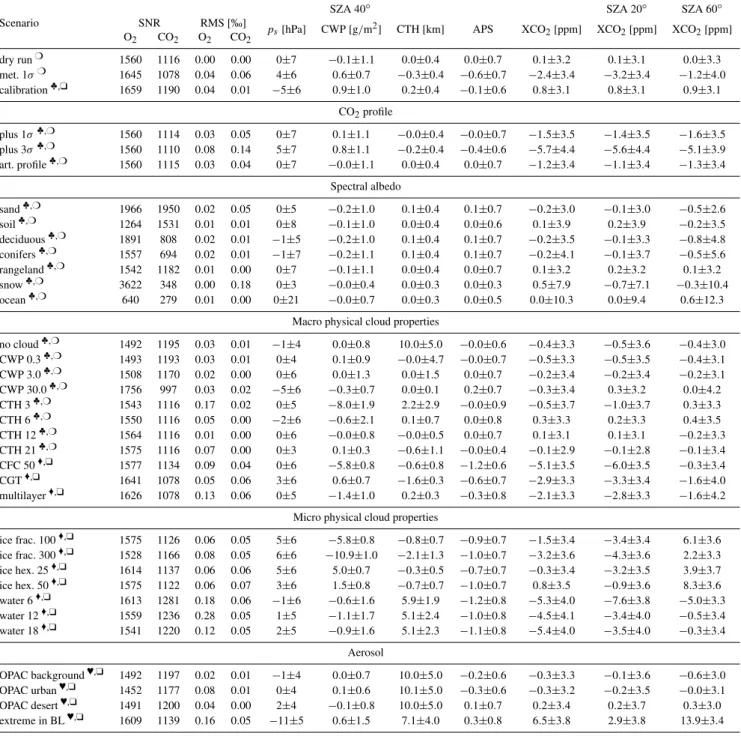
An overview of the results of all test scenarios is given in Table 2 showing the systematic and stochastic XCO2errors
of all scenarios for the solar zenith angles (SZA) 20◦, 40◦, and 60◦. Additionally, the systematic and stochastic errors of the scattering parameters and the surface pressure are given for 40◦SZA. Except for the ”spectral albedo” scenarios, all calculations are performed with an spectrally constant Lam-bertian albedo of 0.2. Table A1 and Table A2 include cor-responding results but for calculations with an albedo of 0.1 and 0.3, respectively.
Note: The stochastic errors represent the a posteriori errors based on the assumed measurement noise and the assumed a priori error covariance matrix. According to Eq. (3.16) of Rodgers (2000), the systematic errors given in Table 2 cor-respond to the smoothing error(A−I)(xt−xa)of the state
vector elements. This applies to all scenarios in which only state vector elements but no parameter vector elements are modified. In these cases, errors due to noise, unknown pa-rameter vector elements, and due to the forward model do not exist.
4.1 The “dry run” scenario
The true state vector of the “dry run” scenario is almost iden-tical to the first guess state vector which is again ideniden-tical to the a priori state vector in almost all elements. Only the con-stant part of the albedo polynomials of the first guess state vector differ slightly from the true state vector as it is esti-mated by the prior first guess albedo retrieval mentioned in Sect. 3.2.2. The “dry run” scenario includes a thin cirrus cloud with a CTH of 10 km, a CWP of 10 g/m2, and a COT at 500 nm of 0.33.
Residuals with relative root mean square (RMS) values be-low 0.005‰ in the O2and CO2region as well as almost no
systematic errors prove that the algorithm is self-consistent (Table 2).
Table 2. Overview of the retrieval performance for 35 test scenarios based on SCIATRAN 3.0 simulations with a modified US-standard atmosphere. For all scenarios, we assume a Lambertian surface with an albedo which is spectrally constant 0.2except for the “spectral albedo” scenarios. The table shows the average signal to noise (SNR) and the residuals relative root mean square (RMS) in both fit windows as well as the main retrieval errors of XCO2, scattering parameters (CWP, CTH, APS), and surface pressure. All errors are given
with systematic error (bias) ±stochastic error. The scenarios are based on the “dry run” scenario (♣), the “met. 1σ” scenario (♦), and the “no cloud” scenario (♥). Some scenarios are intended to quantify the retrievals capability of reproducing modifications of state vector elements (❍). The other scenarios are intended to additionally quantify the retrievals sensitivity to parameter vector elements (❑) (i.e. to a imperfect forward model).
SZA 40◦ SZA 20◦ SZA 60◦
Scenario SNR RMS[‰]
O2 CO2 O2 CO2
ps[hPa] CWP[g/m2] CTH[km] APS XCO2[ppm] XCO2[ppm] XCO2[ppm]
dry run❍ 1560 1116 0.00 0.00 0±7 −0.1±1.1 0.0±0.4 0.0±0.7 0.1±3.2 0.1±3.1 0.0±3.3 met. 1σ❍ 1645 1078 0.04 0.06 4±6 0.6±0.7 −0.3±0.4 −0.6±0.7 −2.4±3.4 −3.2±3.4 −1.2±4.0 calibration♣,❑ 1659 1190 0.04 0.01 −5±6 0.9±1.0 0.2±0.4 −0.1±0.6 0.8±3.1 0.8±3.1 0.9±3.1
CO2profile
plus 1σ♣,❍ 1560 1114 0.03 0.05 0±7 0.1±1.1 −0.0±0.4 −0.0±0.7 −1.5±3.5 −1.4±3.5 −1.6±3.5 plus 3σ♣,❍ 1560 1110 0.08 0.14 5±7 0.8±1.1 −0.2±0.4 −0.4±0.6 −5.7±4.4 −5.6±4.4 −5.1±3.9 art. profile♣,❍ 1560 1115 0.03 0.04 0±7 −0.0±1.1 0.0±0.4 0.0±0.7 −1.2±3.4 −1.1±3.4 −1.3±3.4
Spectral albedo
sand♣,❍ 1966 1950 0.02 0.05 0±5 −0.2±1.0 0.1±0.4 0.1±0.7 −0.2±3.0 −0.1±3.0 −0.5±2.6 soil♣,❍ 1264 1531 0.01 0.01 0±8 −0.1±1.0 0.0±0.4 0.0±0.6 0.1±3.9 0.2±3.9 −0.2±3.5 deciduous♣,❍ 1891 808 0.02 0.01 −1±5 −0.2±1.0 0.1±0.4 0.1±0.7 −0.2±3.5 −0.1±3.3 −0.8±4.8 conifers♣,❍ 1557 694 0.02 0.01 −1±7 −0.2±1.1 0.1±0.4 0.1±0.7 −0.2±4.1 −0.1±3.7 −0.5±5.6 rangeland♣,❍ 1542 1182 0.01 0.00 0±7 −0.1±1.1 0.0±0.4 0.0±0.7 0.1±3.2 0.2±3.2 0.1±3.2 snow♣,❍ 3622 348 0.00 0.18 0±3 −0.0±0.4 0.0±0.3 0.0±0.3 0.5±7.9 −0.7±7.1 −0.3±10.4 ocean♣,❍ 640 279 0.01 0.00 0±21 −0.0±0.7 0.0±0.3 0.0±0.5 0.0±10.3 0.0±9.4 0.6±12.3
Macro physical cloud properties
no cloud♣,❍ 1492 1195 0.03 0.01 −1±4 0.0±0.8 10.0±5.0 −0.0±0.6 −0.4±3.3 −0.5±3.6 −0.4±3.0 CWP 0.3♣,❍ 1493 1193 0.03 0.01 0±4 0.1±0.9 −0.0±4.7 −0.0±0.7 −0.5±3.3 −0.5±3.5 −0.4±3.1 CWP 3.0♣,❍ 1508 1170 0.02 0.00 0±6 0.0±1.3 0.0±1.5 0.0±0.7 −0.2±3.4 −0.2±3.4 −0.2±3.1 CWP 30.0♣,❍ 1756 997 0.03 0.02 −5±6 −0.3±0.7 0.0±0.1 0.2±0.7 −0.3±3.4 0.3±3.2 0.0±4.2
CTH 3♣,❍ 1543 1116 0
.17 0.02 0±5 −8.0±1.9 2.2±2.9 −0.0±0.9 −0.5±3.7 −1.0±3.7 0.3±3.3 CTH 6♣,❍ 1550 1116 0.05 0.00 −2±6 −0.6±2.1 0.1±0.7 0.0±0.8 0.3±3.3 0.2±3.3 0.4±3.5 CTH 12♣,❍ 1564 1116 0.01 0.00 0±6 −0.0±0.8 −0.0±0.5 0.0±0.7 0.1±3.1 0.1±3.1 −0.2±3.3 CTH 21♣,❍ 1575 1116 0.07 0.00 0±3 0.1±0.3 −0.6±1.1 −0.0±0.4 −0.1±2.9 −0.1±2.8 −0.1±3.4 CFC 50♦,❑ 1577 1134 0.09 0.04 0±6 −5.8±0.8 −0.6±0.8 −1.2±0.6 −5.1±3.5 −6.0±3.5 −0.3±3.4 CGT♦,❑ 1641 1078 0.05 0.06 3±6 0.6±0.7 −1.6±0.3 −0.6±0.7 −2.9±3.3 −3.3±3.4 −1.6±4.0 multilayer♦,❑ 1626 1078 0.13 0.06 0±5 −1.4±1.0 0.2±0.3 −0.3±0.8 −2.1±3.3 −2.8±3.3 −1.6±4.2
Micro physical cloud properties
ice frac. 100♦,❑ 1575 1126 0.06 0.05 5±6 −5.8±0.8 −0.8±0.7 −0.9±0.7 −1.5±3.4 −3.4±3.4 6.1±3.6 ice frac. 300♦,❑ 1528 1166 0.08 0.05 6±6 −10.9±1.0 −2.1±1.3 −1.0±0.7 −3.2±3.6 −4.3±3.6 2.2±3.3 ice hex. 25♦,❑ 1614 1137 0.06 0.06 5±6 5.0±0.7 −0.3±0.5 −0.7±0.7 −0.3±3.4 −3.2±3.5 3.9±3.7 ice hex. 50♦,❑ 1575 1122 0.06 0.07 3±6 1.5±0.8 −0.7±0.7 −1.0±0.7 0.8±3.5 −0.9±3.6 8.3±3.6 water 6♦,❑ 1613 1281 0.18 0.06 −1±6 −0.6±1.6 5.9±1.9 −1.2±0.8 −5.3±4.0 −7.6±3.8 −5.0±3.3 water 12♦,❑ 1559 1236 0.28 0.05 1±5 −1.1±1.7 5.1±2.4 −1.0±0.8 −4.5±4.1 −3.4±4.0 −0.5±3.4 water 18♦,❑ 1541 1220 0.12 0.05 2±5 −0.9±1.6 5.1±2.3 −1.1±0.8 −5.4±4.0 −3.5±4.0 −0.3±3.4
Aerosol
OPAC background♥,❑ 1492 1197 0.02 0.01 −1±4 0.0±0.7 10.0±5.0 −0.2±0.6 −0.3±3.3 −0.1±3.6 −0.6±3.0 OPAC urban♥,❑ 1452 1177 0.08 0.01 0±4 0.1±0.6 10.1±5.0 −0.3±0.6 −0.3±3.2 −0.2±3.5 −0.0±3.1 OPAC desert♥,❑ 1491 1200 0.04 0.00 2±4 −0.1±0.8 10.0±5.0 0.1±0.7 0.2±3.4 0.2±3.7 0.3±3.0
extreme in BL♥,❑ 1609 1139 0
.16 0.05 −11±5 0.6±1.5 7.1±4.0 0.3±0.8 6.5±3.8 2.9±3.8 13.9±3.4
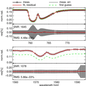
4.2 The “met. 1σ” scenario
The meteorological parameters (temperature shift, H2O
scal-ing, APS, CWP, CTH,ps, and CO2mixing ratio) of the true
state vector of the “met. 1σ” scenario differ from the cor-responding values of the a priori state vector by 0.5 to 1.0
sigma a priori uncertainty. The “met. 1σ” scenario includes a thin cirrus cloud with a CTH of 15 km, a CWP of 15 g/m2, and a COT at 500 nm of 0.49.
0.00 0.05 0.10 0.15 0.20
760 765 770
−0.10 0.00 0.10
res[%]
norm.rad.
SNR: 1645
RMS: 4.48e−03%
0.09 0.11 0.13
1560 1570 1580 1590
wavelength [nm] −0.20
0.00 0.20
res[%]
norm.rad.
SNR: 1078
RMS: 5.86e−03% meas. fit, residual
meas. err. first guess
Fig. 7. O2and CO2 fit windows with simulated measurements,
first guess, fitted sun-normalized radiation, residual and simulated measurement uncertainty for the “met. 1σ” scenario at 40◦solar zenith angle.
reduction are given for this scenario in Table 3. The cor-responding spectral fits in both fit windows as well as their residuals are plotted in Fig. 7.
We find large uncertainty reductions greater than 0.88 for the albedo parameters, wavelength shift, and FWHM within the O2 spectral region. The corresponding values of the
CO2spectral region are somewhat smaller but always greater
equal 0.69. Temperature shift and H2O scaling are retrieved
with low systematic biases and error reductions of 0.67 and 0.79 despite rather narrow a priori constraints.
In contrast to this, the APS retrieval, with an uncertainty reduction of only 0.32, seems to be dominated by the a pri-ori even though the corresponding constraints are weak. Ac-cordingly, we find a large stochastic error of 0.7 and a large systematic bias of−0.6 which brings the retrieval close to the a priori value. This can be explained by the following: The aerosol profile has its maximum in the boundary layer and scattering and absorption features of aerosol vary only slowly in the relatively narrow fit windows. Therefore, it is not surprising that the shape of the APS weighting function has similarities to the surface pressure weighting function. Additionally, the sensitivity to APS is very low due to very low absolute values of the APS weighting function. For both points see Fig. 2.
Compared to APS, the error reduction of CWP and CTH is much higher (>0.9). Referring to Fig. 2, the shape of the CWP weighting function strongly depends on the specific scenario which can cause ambiguities, problems of finding
300 400 500 600
CO2 mixing ratio [ppm]
1.0 0.8 0.6 0.4 0.2 0.0
pressure [p
s
]
CO2 profile plus 1σ
CO2 profile plus 3σ
artificial CO2 profile
a priori CO2 profile
true true true xa
retrieved retrieved retrieved 1σ
Fig. 8. Retrieved and true CO2mixing ratio profiles of the three
“CO2profile” scenarios.
suitable first guess values, and problems of the convergence behavior. The retrieval’s sensitivity to CWP and CTH is de-scribed in more detail in Sect. 4.6.
The surface pressure is retrieved with a bias of 4 hPa, a stochastic error of 6 hPa and an error reduction of 0.80. As the CO2 layered weighting functions look very similar
and as the a priori knowledge shows strong inter-correlation between the layers, the retrieved profile has also strongly correlated layers. Additionally, the retrieval shows a very low error reduction especially in the stratosphere resulting in a degree of freedom for signal of 1.07 for the whole pro-file. This means that only one independent information can be retrieved about the profile. The shape of the profile re-mains strongly dominated by the a priori statistics. See also Sects. 4.4 and 4.9.
The “met. 1σ” scenario serves as basis for several other scenarios which are mainly intended to quantify the retrievals performance under more realistic conditions including also unknown parameter vector elements, i.e. an imperfect for-ward model.
4.3 Calibration
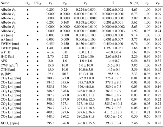
Table 3. Detailed retrieval results of the “met. 1σ” scenario for each state vector element and for the resulting XCO2. The meaning of the columns from left to right is: 1) name of the state vector element, 2+3) weighting function with non-zero elements in the O2and CO2 fit window, respectively, 4) true statext, 5) first guess statex0, 6) a priori statexa±uncertainty, 7) retrieved statexˆ ±stochastic error, 8)
information contentH, 9) degree of freedom for signalds, 10) uncertainty reductionrσ Note:xt,x0,xa,xˆ, and the corresponding errors
are rounded to the same number of digits within each line.
Name O2 CO2 xt x0 xa xˆ H [bit] ds rσ
AlbedoP0 • 0.200 0.224 0.224±0.050 0.202±0.002 4.65 1.00 0.96 AlbedoP1 • 0.0000 0.0000 0.0000±0.0100 0.0000±0.0001 6.73 1.00 0.99 AlbedoP2 • 0.0000 0.0000 0.0000±0.0010 0.0000±0.0001 3.09 0.99 0.88 AlbedoP0 • 0.200 0.168 0.168±0.050 0.201±0.001 5.62 1.00 0.98 AlbedoP1 • 0.0000 0.0000 0.0000±0.0100 0.0000±0.0002 5.63 1.00 0.98 AlbedoP2 • 0.0000 0.0000 0.0000±0.0010 0.0001±0.0003 1.92 0.93 0.74
1λ[nm] • 0.000 0.000 0.000±0.100 0.000±0.000 9.14 1.00 1.00 1λ[nm] • 0.000 0.000 0.000±0.100 0.001±0.007 3.77 0.99 0.93 FWHM[nm] • 0.450 0.450 0.450±0.050 0.450±0.000 6.76 1.00 0.99 FWHM[nm] • 1.400 1.400 1.400±0.100 1.397±0.031 1.68 0.90 0.69 1T[K] • • −0.6 0.0 0.0±1.1 −0.8±0.4 1.62 0.89 0.67 H2O[‰] • • 2.70 2.22 2.22±0.86 2.65±0.18 2.26 0.96 0.79
APS • • 2.0 1.0 1.0±1.0 1.4±0.7 0.56 0.54 0.32
CWP [g/m2] • • 15.0 10.0 5.0±10.0 15.6±0.7 3.85 1.00 0.93 CTH[km] • • 15.0 10.0 10.0±5.0 14.7±0.4 3.59 0.99 0.92 ps[hPa] • • 981 1013 1013±30 985±6 2.33 0.96 0.80
CO2L9[ppm] • 380.9 373.0 372.9±8.0 375.4±7.5 0.01 0.01 0.06 CO2L8[ppm] • 384.5 375.6 375.7±9.0 378.3±8.5 0.02 0.02 0.06 CO2L7[ppm] • 385.1 376.4 376.4±8.6 380.9±7.3 0.03 0.04 0.16 CO2L6[ppm] • 386.6 376.8 376.8±10.0 383.0±7.9 0.03 0.04 0.21 CO2L5[ppm] • 387.9 377.0 377.0±11.1 384.0±8.7 0.03 0.05 0.22 CO2L4[ppm] • 388.9 377.0 377.0±12.0 384.7±9.4 0.04 0.05 0.22 CO2L3[ppm] • 390.0 377.1 377.1±13.1 385.7±10.2 0.04 0.05 0.22 CO2L2[ppm] • 394.7 377.3 377.3±18.8 394.7±9.8 0.08 0.10 0.48 CO2L1[ppm] • 409.3 377.6 377.6±36.4 411.5±18.5 0.17 0.21 0.49 CO2L0[ppm] • 448.0 380.2 380.2±81.8 453.6±42.0 0.50 0.50 0.49
XCO2[ppm] 395.6 376.8 376.8±15.6 393.2±3.4 2.46 1.07 0.78
by a factor by 10%. This primarily affects the retrieved 0th order albedo polynomials which are approximately 10% too large. The weighting function of the 0th order albedo polynomial shows similarities with other weighting functions (Fig. 4) which affects the retrieval errors of other parameters. However, the systematic errors of XCO2remain smaller than
1 ppm.
4.4 CO2profile
The detailed results of the “met. 1σ” scenario, given in Ta-ble 3, already show that it is not possiTa-ble to retrieve much information about the profile shape. Figure 8 shows the retrieved CO2 profiles of the “plus 1σ”, “plus 3σ”, and
“art. profile” CO2profile scenarios. The three scenarios
dif-fer from the “dry run” scenario only by a modified (true) CO2
profile.
The “plus 1σ” scenario has a true CO2profile which
dif-fers from the a priori profile by an enhancement of 1σa priori uncertainty in each layer. We find a slight overestimation of
the CO2mixing ratio in the boundary layer, an almost
neu-tral behavior between 0.8ps and 0.3ps, and a slight
underes-timation in the stratosphere. The resulting XCO2has a bias
of−1.5 ppm and a stochastic error of 3.5 ppm for 40◦SZA (Table 2).
In the case of the “plus 3σ” scenario, the observed effects become more pronounced. We find a week overestimation in the boundary layer, a week underestimation between 0.8ps
and 0.3ps, and a clear underestimation in the stratosphere.
The resulting XCO2has a bias of−5.7 ppm and a
stochas-tic error of 4.4 ppm (Table 2). Even though this scenario is a clear outlier in terms of the a priori statistics, the al-gorithm is still able to retrieve XCO2with a systematic
ab-solute error of 1.5%. This means that the XCO2 retrieval
In order to illustrate that it is actually not possible to re-trieve the shape of the CO2profile, we confront the retrieval
with an artificial profile with an almost constant mixing ratio of 380 ppm in all layers except the third layer having a mix-ing ratio of about 495 ppm. In this case, the retrieved CO2
profile follows not the true profile. In fact, the retrieved pro-file still adopts the shape from the a priori information even though the direction of the profile modification is retrieved correctly. However, the a priori information of the CO2
pro-file, which we generate from CarbonTracker data, hint that the profile shape is already relatively well known before the measurement (Fig. 6). Therefore, it is most unlikely that sce-narios like the “art. profile” scenario occur in reality.
Note that the systematic errors shown in this subsection correspond to the CO2profile smoothing error.
4.5 Spectral albedo
Unfortunately, the spectral albedo cannot be assumed to be constant within the O2and CO2fit window. In the worst case,
the spectral shape of the albedo would be highly correlated with the surface pressure or CO2weighting function. In this
case, errors of the retrieved surface pressure or CO2mixing
ratios would be unavoidable. However, this is most unlikely in reality.
As illustrated in Fig. 5, the albedo of typical surface types is spectrally smooth and only slowly varying within the fit windows. This applies especially to satellite pixels with large foot print size consisting of a mixture of surface types. Therefore, we assume that the albedo can be approximated within each fit window with a 2nd order polynomial. In or-der to make a perfect retrieval with no remaining residuals theoretically possible, we fit a 2nd order polynomial in both fit windows to the spectral albedos given in Fig. 5. We use these polynomials as true spectral albedo for the albedo sce-narios “sand”, “soil”, “deciduous”, “conifers”, “rangeland”, “snow”, and “ocean”. All other elements of the state vector are identical to those of the “dry run” scenario.
Table 2 shows that the systematic XCO2 errors of these
scenarios are all between−0.8 and 0.6 ppm, most of them close to zero. We observe almost no systematic errors for the surface pressure. According to the large differences of the tested albedos, SNR values vary from 640 to 3622 in the O2
fit window and from 279 to 1950 in the CO2fit window.
We find the lowest stochastic XCO2errors for the “sand”
scenario. This scenario has a relatively high albedo of about 0.3 in the O2and 0.5 in the CO2fit window. For this reason
the corresponding SNR values are also relatively large which is essential for low stochastic errors.
The largest SNR values are observed in the O2 fit
win-dow for the “snow” scenario because of the high reflectivity of snow in this spectral region. Due to the higher spectral resolution, stronger absorption features, and most times bet-ter SNR values in the O2 fit window, the surface pressure
retrieval is dominated by the O2fit window. For this reason,
we observe a distinctively smaller stochastic surface pressure error of 3 hPa for this scenario. Nevertheless, the stochastic XCO2error of this scenario is quite large with about 8 ppm.
This can be explained by a very low SNR value in the CO2
fit window caused by a very low reflectivity of snow in this spectral region.
The “ocean” scenario has the lowest albedo and there-fore the lowest SNR value in the O2 and CO2 fit window.
Consequently, we here observe the largest stochastic errors of 21 hPa for the surface pressure and of about 10 ppm for XCO2. Comparing these values with the uncertainty of the
prior knowledge shows that only very little information about XCO2can be obtained over snow covered or ocean surfaces. 4.6 Macro physical cloud parameter
Within the scenarios “no cloud”, “CWP 0.3” to “CWP 30.0”, we test the retrievals ability to retrieve CWP of an ice cloud of fractal particles with 50 µm effective radius (as defined in the parameter vector). All other state vector elements are de-fined as in the “dry run” scenario. As implied by the name of these scenarios, the ice content of the analyzed clouds amounts to 0.0, 0.3, 3.0, and 30.0 g/m2. The correspond-ing cloud optical thicknesses of these scenarios are about 0.00, 0.01, 0.10, and 1.00. Note, in this context, specify-ing only the optical thickness is not appropriate to describe the scattering behavior of a cloud. Knowledge about phase function, extinction, and absorption coefficients is required in order to make the optical thickness a meaningful quantity. The SNR values of the “no cloud” and “CWP 0.3” scenar-ios is almost identical and there are only weak differences to the “CWP 3.0” scenario. This indicates that the clouds of these cases are extremely transparent and most likely not visible for the human eye. In contrast to this, the SNR of the “CWP 30.0” scenario increases within the O2fit window.
Within the CO2fit window, the effect of enhanced
backscat-tered radiation is balanced by the strong absorption of ice in this spectral region. We observe nearly no systematic errors of the retrieved surface pressure except for the “CWP 30.0” scenario which results in a bias of −5 hPa. The CWP re-trieval is almost bias free compared to its stochastic error for all analyzed solar zenith angles. The same applies to the re-trieved CTH of the “CWP” scenarios. For the “no cloud” scenario, the unmodified a priori value is retrieved without any error reduction which is reasonable. The stochastic CTH error reduces for CWP values greater than 3.0 g/m2. The systematic absolute XCO2error of these scenarios is less or
equal 0.5 ppm whereas the stochastic error is in the range of 3.0 and 4.2 ppm. In contrast to this, a WFM-DOAS like retrieval systematically overestimates XCO2 by 3, 33, and
30.0 g/m2 especially for large solar zenith angles. In such cases, the algorithm is often not able to discriminate between a thick cloud or an extremely low surface pressure.
Analogous to the “CWP” scenarios, the “CTH” scenarios are identical to the “dry run” scenario except for the cloud top height which varies between 3, 6, 12, and 21 km. CWP, CTH, and APS are retrieved nearly bias free for the “CTH 6”, “CTH 12”, and “CTH 21” scenario. The systematic XCO2
error of these scenarios is also comparatively low with values between−0.2 and 0.4 ppm. Only the “CTH 3” scenario pro-duces larger systematic errors of CWP and CTH. Addition-ally, the systematic XCO2error of this scenario is slightly
larger with values up to−1.0 ppm. This behavior may be ex-plained by the fact that APS, and especially CTH and CWP weighing functions become more and more similar for low clouds.
Up to this point, we only tested the retrieval’s ability to reproduce modifications to state vector elements. However, and as mentioned before, especially in respect to scattering, three state vector elements are by far not enough to entirely define the radiative transfer. For this reason, we analyze the retrieval’s sensitivity to different parameter vector elements within the following scenarios. At this, we put the emphasis on properties of thin cirrus clouds. In the context of macro physical cloud parameters we estimate the retrieval’s sensi-tivity to cloud fractional coverage of 50% (“CFC 50” sce-nario), cloud geometrical thickness (“CGT” scesce-nario), and multilayer clouds (“multilayer” scenario). These three sce-narios are based on the “met. 1σ” scenario. They only differ from their reference scenario by modified cloud properties.
The radiation of the “CFC 50” scenario is an average of the radiation of the “met. 1σ” scenario with and without cloud. We observe a systematic CWP error being 6.4 g/m2smaller than the corresponding error of the “met. 1σ” reference sce-nario. This can be explained with the total ice content of the “CFC 50” scenario which is 7.5 but not 15 g/m2. We re-trieve XCO2values systematically differing in the range of
−2.8 and 0.9 ppm from those of the reference scenario. This implies that the errors induced by fractional cloud coverage may also depend on CWP because the modeled cloud ap-pears thicker or thinner under different solar zenith angles. The total XCO2 errors are here in the range of −6.0 and
−0.3 ppm.
The “CGT” scenario differs from the reference scenario only by the cloud geometrical thickness that is 2.5 km com-pared to 0.5 km for the reference scenario. The results of this scenario are very similar to the reference results. Solely, the retrieved CTH is systematically 1.3 km lower. Due to the larger geometrical thickness and identical ice content at the same time, the particle density is lower. For this reason, the effective penetration depth in this cloud is larger which can explain the differences of the retrieved CTH.
The “multilayer” scenario includes two clouds with iden-tical ice particles and ideniden-tical geometrical thickness of 0.5 km. The lower CTH is 8 km whereas the upper CTH is
12 km. The corresponding “true” value, which is the basis for the calculation of the CTH bias in Table 2, amounts to 10 km. The results of this scenario are also comparable with the results of the reference scenario. Systematic XCO2
dif-ferences compared to the reference scenario are in the range of −0.4 and 0.4 ppm. The retrieved CTH lies between the simulated clouds and is 0.2 km larger than the average CTH of both cloud layers.
4.7 Micro physical cloud parameter
Within this section we estimate the retrieval’s sensitivity to cloud micro physical properties. This means, we confront the retrieval with clouds consisting of particles differing from those defined in the parameter vector.
The information about the three retrieved scattering pa-rameters CWP, CTH, and APS can nearly entirely be at-tributed to the O2fit window. Scattering properties are
de-fined within the state vector solely by these three parameters. The whole micro physical cloud and aerosol properties like phase function, extinction, and absorption coefficients are only defined in the parameter vector. Unfortunately, these micro physical properties are not known and also not con-stant in reality and the values that we define in the parameter vector are obviously only a rough estimate.
Let us first consider only the O2 fit window and assume
that extinction and absorption coefficients as well as phase function of the scattering particles are constant in this spec-tral region. Let us now assume two clouds having phase functions which differ only by a factor (or an offset within a logarithmic plot) outside the forward peak. In such case, the CWP retrieval would be ambiguous in respect to the mi-cro physical properties and consequently, correct CWP val-ues are only retrievable if the scattering particles are known. Referring to Fig. 3, the volume scattering functions within the O2fit window of e.g. fractal ice crystals of different size
show such similarities. This means that in the case of un-known particles, it is hardly possible to retrieve the true CWP from measurements in the O2fit window only. The retrieved