ISSN: 1809-4430 (on-line)
_________________________
1 Licenciada em Matemática, Prof. Doutora, Centro de Ciências Exatas e Tecnológicas (CCET), Programa de Pós-Graduação em Engenharia Agrícola (PGEAGRI), UNIOESTE/Cascavel - PR, Fone: (45) 32207320, [email protected]
2 Agrônomo, Prof. Doutor, Departamento de Estatística, UFPR/Curitiba – PR, [email protected]
3 Estatístico, Prof. Doutor, Centro de Ciências Exatas e Tecnológicas (CCET), Programa de Pós-Graduação em Engenharia Agrícola (PGEAGRI), UNIOESTE/Cascavel - PRProdutividade Científica CNPq, [email protected]
4 Licenciada em Matemática, Doutora em Estatística, UFPE/Recife - PE, [email protected] Recebido pelo Conselho Editorial em: 24-11-2014
SOYBEAN YIELD MAPS USING REGULAR AND OPTIMIZED SAMPLE WITH DIFFERENT CONFIGURATIONS BY SIMULATED ANNEALING
Doi:http://dx.doi.org/10.1590/1809-4430-Eng.Agric.v36n1p 114-125/2016
LUCIANA P. C. GUEDES1, PAULO J. RIBEIRO JUNIOR2, MIGUEL A. URIBE-OPAZO3,
FERNANDA DE BASTIANI4
ABSTRACT: This study aimed to compare thematic maps of soybean yield for different sampling grids, using geostatistical methods (semivariance function and kriging). The analysis was performed with soybean yield data in t ha-1 in a commercial area with regular grids with distances between points of 25x25 m, 50x50 m, 75x75 m, 100x100 m, with 549, 188, 66 and 44 sampling points respectively; and data obtained by yield monitors. Optimized sampling schemes were also generated with the algorithm called Simulated Annealing, using maximization of the overall accuracy measure as a criterion for optimization. The results showed that sample size and sample density influenced the description of the spatial distribution of soybean yield. When the sample size was increased, there was an increased efficiency of thematic maps used to describe the spatial variability of soybean yield (higher values of accuracy indices and lower values for t he sum of squared estimation error). In addition, more accurate maps were obtained, especially considering the optimized sample configurations with 188 and 549 sample points.
KEYWORDS: accuracy indices, optimization, sampling grids, spatial variability.
MAPAS DA PRODUTIVIDADE DA SOJA USANDO CONFIGURAÇÕES AMOSTRAIS REGULARES E OTIMIZADAS PELA TÊMPERA SIMULADA
RESUMO: Neste trabalho, teve-se o objetivo de estudar e comparar mapas temáticos da produtividade da soja para diferentes grades amostrais, utilizando métodos geoestatísticos (função semivariância e krigagem). A análise foi realizada com dados da produtividade de soja em t ha-1 numa área comercial com grades regulares e distâncias entre pontos de 25x25 m, 50x50 m, 75x75 m e 100x100 m, com 549; 188; 66 e 44 pontos amostrais, respectivamente, e dados obtidos pelo monitor de colheita. Também foram gerados esquemas amostrais otimizados, com o algoritmo chamado Têmpera Simulada, usando a maximização da medida de acurácia exatidão global, como critério de otimização. Foi verificado que fatores como o tamanho da amostra e a densidade amostral influenciaram na descrição da distribuição espacial da produtividade da soja feita por meio dos mapas temáticos. Quando se aumentou o tamanho amostral, houve aumento da eficiência dos mapas temáticos quanto à descrição da variabilidade espacial da produtividade da soja (maiores valores dos índices de acurácia e os menores valores para a soma quadrada do erro de estimação). Além disso, os mapas mais acurados foram obtidos considerando as configurações amostrais otimizadas com 188 e 549 pontos amostrais.
INTRODUCTION
With the advance of mechanized technologies and the growth of worldwide agricultural production, many researchers have been investigating the production process searching for sustainable farming practices that can radically improve agricultural production, for instance by reducing the use of agricultural inputs. In particular, soybean production is of extreme economic importance to Brazil. In the 2010/11 crop-year, global soybean yield was 263.7 million tonnes, with a planted area of 103.5 million hectares, where Brazil is the second largest soybean producer (USDA, 2011). In the same year, Brazil had an average yield of 3.125 t ha-1 over an area greater than 24 million hectares, totaling a yield of 75 million tonnes (CONAB, 2011).
Research on the spatial dependence structure of agricultural georeferenced variables, such as chemical and physical soil properties and crop yield, is an analysis tool which provides information to support a decision in favour of better management of production areas (BORSSOI et al., 2011; GREGO et al., 2011; URIBE-OPAZO et al., 2012; NESI et al., 2013; ASSUMPÇÃO et al., 2014; BERNARDI et al., 2014). This can be accomplished by means of geostatistical techniques that retrieve from a set of sample elements, information about the spatial variation of the phenomenon in the whole area through the construction of thematic maps of variability (DIGGLE & RIBEIRO JUNIOR, 2007).
The number of sample elements available to conduct research on the spatial dependent variables and their respective sample configuration, may affect the description of the spatial dependence structure, or more, the spatial estimates of non-sampled values obtained by the kriging interpolation technique, and consequently the reliability of the results shown by the thematic map (URIBE-OPAZO et al., 2007; COELHO et al., 2009; ODA-SOUZA et al., 2010; GUEDES et al., 2011; RIFFEL et al., 2012; SOUZA et al., 2014).
When financial resources are limited, the definition of the shape and size of sampling strategy to be used to study the spatial dependence structure are crucial, in an effort to both minimize operating costs and maximize the results of spatial prediction. Thus, it is necessary to study how the sampling strategy used in the study area affects the estimation of the parameters of the spatial model that describes the spatial dependence structure of the georeferenced variable, the spatial estimation of this variable in non-observed locations and, as a consequence, the thematic maps to be generated for such estimation (SPOCK & HUSSAIN, 2012).
In this context, the aim of this study was to evaluate the influence of different sampling grids on the description of the spatial dependence structure of soybean yield. The configurations used in this study were regular grids and optimized configurations by the optimization method called Simulated Annealing, both with different sample densities.
MATERIAL AND METHODS
The soybean productivity (t ha-1) data used in this study were collected in a commercial area
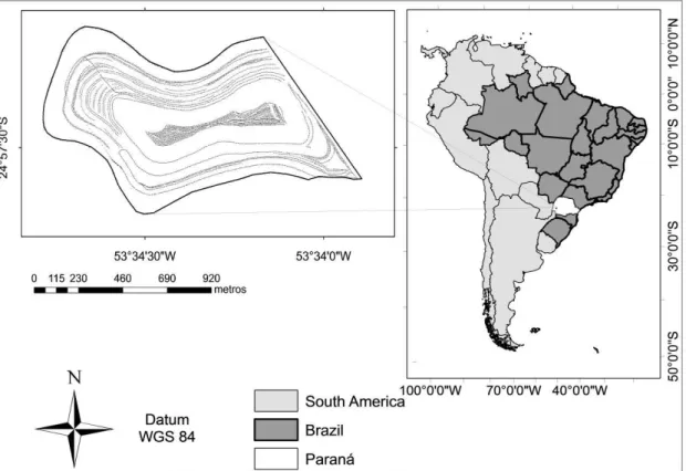
of 57.16 ha, located in Cascavel city, in western region of Paraná State, Brazil. The area has approximate geographic coordinates of 24.95° S and 53.57° W, with an average elevation of 650 m above sea level (Figure 1). The soil of the region is classified as Oxisols with clayey texture and deep soils with good water storage capacity, porosity and permeability. The climate in the region is very wet and classified as mesothermal, Cfa (Köeppen), with average annual temperature of 21ºC (IAPAR, 2007).
FIGURE 1. Location of the commercial area and database generated by harvest monitors totaling
7588 points.
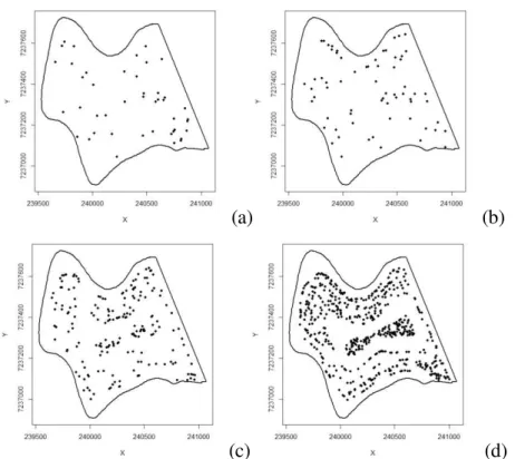
(a) (b)
(c) (d)
FIGURE 2. Location of sampling points of regular grids with (a) 44, (b) 66, (c) 188 and (d) 549 sampling points.
function. The criteria for model selection were cross-validation and maximum value of the log-likelihood function (LML).
These estimates also allowed to obtain the relative nugget effect
, which represents the intensity of spatial dependence (CAMBARDELLA et al., 1994).
Considering the locations of the original mesh (7588 points), yield values in these locations were estimated by ordinary kriging method, using values as the results of each regular grid (44, 66, 188 and 549 sampling points) and estimating the parameters selected by the models selection criteria.
The estimated yield values for the grids 100x100 m, 75x75 m, 50x50 m and 25x25 m were compared with the actual yield values obtained by the harvest monitor, using the sum of squared errors (SQE) of the spatial estimation and the accuracy measures described in Table 1.
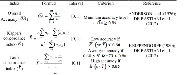
TABLE 1. Accuracy measures.
Index Formula Interval Criterion Reference
Overall
Accuracy ( ) [0, 1] Minimum accuracy level
if
ANDERSON et al. (1976); DE BASTIANI et al.
(2012)
Kappa’s
concordance index ( )
m i i i m i i i m i ii n n n n n n n 1 2 11 [0, 1]
Low accuracy if
Average accuracy if
High accuracy if
KRIPPENDORFF (1980); DE BASTIANI et al.
(2012)
Tau’s
concordance index ( )
m m n T m i ii 1 1 1 1 ^
[0,1]To calculate the accuracy measures shown in Table 1, the error matrix (Table 2) as described by DE BASTIANI et al. (2012) was adapted in this study, considering ten classes of intervals of values (m = 10). Each element of the error matrix ( ) represents the number of estimations classified into class i ( ) of the model map (set of estimated values at the locations of the
original mesh, obtained through the sampling points of the study grids) and class j( ) of
the reference map (values of the original mesh, obtained by the harvest monitor).
This study also developed optimized sample configurations with the same sample sizes used in regular grids, for its efficiency in spatial prediction at locations not sampled by the method called Simulated Annealing (SA) (RUIZ-CÁRDENAS et al., 2010), using the accuracy measure called Overall accuracy as an objective function to be maximized (Table 1).
The algorithm that determined the optimal sample configuration by Simulated Annealing was implemented through the following steps:
TABLE 2. General error matrix.
Reference map
Model map 1 2 m Total
1 n11 n12 n1m n1
2 n21 n22 n2m n2
m nm1 nm2 nmm nm
Total n1 n2 nm n
: number of estimations classified into to class i of the model map and class j of the reference map; : number of estimations
classified into class i of the model map; : number of estimations classified into class j of the reference map; : number of
estimations classified into the same class in both maps; : total values in the original mesh (harvest monitor); : number of classes of error matrix.
Step 1: A random sampling configuration Si with reduced size d0 (44, 66, 188 and 549
sampling points) was selected from the initial mesh.
Step 2: For this sample configuration, a spatial model was fitted by maximum likelihood method, and spatial estimation was performed of yield values at the locations of the original mesh, using the geostatistical interpolation technique called kriging. Next, the objective function was calculated forSi .
Step 3: A new random sampling configuration Si1 was obtained, from the original mesh, and
the objective function was calculated for Si1.
Step 4: The variation of the objective function that occurred between the two sampling schemes was calculated, expressed by i f(Si1) f(Si). The new solution Si1will be accepted
with the probability described in [eq. (1)]:
exp , if 0 .
0 if
, 1
accept 1
i i i i i t S
P (1)
Step 5: The optimization process was completed if the stopping criterion was met. Otherwise, the value of the current temperature was decreased by the cooling schedule described in step 0,
1
i
i was calculated, and step 3 was followed again.
For optimized sample configurations, a spatial model was fitted, following the criteria of cross-validation and LML. Then, based on the estimation of the spatial model and the optimized sample configuration, the soybean yield value was estimated at the locatio ns of the original mesh by the ordinary kriging method.
The estimated yield values for optimized grids were compared with the actual yield values, obtained by the harvest monitor, using the SQE of the spatial estimation and by the accuracy measures described in Table 1.
Regular sampling grids with different sample densities were compared with the sampling grids generated by the optimization process, considering the same sample sizes of regular grids. These sample configurations were compared for the following measures: estimates of accuracy measures described in Table 1, the SQE of spatial estimation and estimates of the parameters of the spatial model.
estimation, fitting of models, spatial estimation and development of the optimization routine. This software program is open source and have GPL (General Public license).
RESULTS AND DISCUSSION
Figure 3 shows the locations of the sampling configurations optimized for Simulated Annealing, considering the same sampling densities of regular grid (Figure 2). Comparing the arrangement of the points, between the regular and optimized grids, it is noted that the arrangement of sampling points in the optimized sampling settings shows that there is an attempt of the optimization process to distribute the points to gain a better coverage of the study area. The same results were observed in simulated datasets and chemical soil properties by GUEDES et al. (2011). Moreover, it is observed that with increasing sample size, there is a similarity between optimized sampling settings and regular grids as for the arrangement of the points.
(a) (b)
(c) (d)
FIGURE 3. Location of sampling configurations obtained by optimization with (a) 44, (b) 66, (c) 188 and (d) 549 sampling points.
Table 3 shows descriptive statistics of the variable soybean yield in t ha-1, for the different sampling grids analyzed, for the optimized sample configurations and for data from the harvest monitor.
It is important to note that some of these descriptive statistics were similar for all sampling grids and for the harvest monitor. The results show that soybean yield, at the different sampling grids, obtained by the harvest monitor showed low dispersion (SD) and homogeneity in the
frequency distribution of data from different sampling grids, with low (CV ≤ 10%, GOMES, 2000) and medium (10 % < CV ≤ 20%, GOMES, 2000) dispersions.
The estimates presented for these models showed that there is a similarity in the estimates of the nugget effect and their standard deviations in all sample configurations and densities. It was also observed that most models fitted to different sampling patterns showed moderate spatial dependence (25% ≤ RNE ≤ 75%; CAMBARDELLA et al, 1994), with the exception of the model fitted to the data of the regular grid with the lowest sample size (44 points), which showed weak spatial dependence (RNE > 75%; CAMBARDELLA et al, 1994).
TABLE 3. Summary of statistics for the four regular grids analyzed, for the harvest monitor and for the optimized sample configurations.
Statistics 25x25 50x50 75x75 100x100 Regular grids Harvest monitor Optimized configurations
Nº samples 549 188 66 44 7582 549 188 66 44
Mean 3.25 3.27 3.22 3.28 3.23 3.29 3.30 3.26 3.38
Median 3.26 3.28 3.19 3.32 3.27 3.31 3.32 3.21 3.41
Q1 3.00 3.00 2.95 3.11 2.98 3.04 3.09 2.95 3.21
Q3 3.54 3.55 3.48 3.49 3.55 3.57 3.56 3.51 3.60
Minimum 1.56 1.63 2.09 2.26 0.68 1.55 1.95 2.69 2.03
Maximum 4.36 4.17 4.09 3.80 4.99 4.99 4.21 4.13 4.08
SD 0.40 0.45 0.38 0.32 0.47 0.41 0.38 0.37 0.36
CV (%) 12.36 12.27 11.71 9.72 14.50 12.43 11.66 11.40 10.60
Q1: 1st quartile; Q3: 3rd quartile; SD: standard deviation; CV: coefficient of variation.
The weak spatial dependence obtained for the data sets with the smallest sample size may have been influenced by the small sample size. This result corroborates the study of URIBE-OPAZO et al. (2007), which compared regular sampling grids with different sample densities and different methods of estimation of the spatial model, and found that the estimation of the parameters that describe the spatial dependence structure of a georeferenced variable, depends not only on the estimation method but also on the number of samples used for geostatistical analysis.
TABLE 4. Parameters estimates for the spatial models, where the standard deviation values of such estimates are shown in parentheses.
Grids (nº samples) Model C0 C1 RNE (%) a
100x100(44) Matérn (k=2) (0.0551) 0.0829 (0.0509) 0.0163 83.57 (597.89) 284.54
75x75(66) Matérn (k=2) (0.0396) 0.0783 (0.0319) 0.0578 57.53 (116.90) 283.60
50x50(188) Matérn (k=2) (0.0182) 0.1090 (0.0083) 0.0496 68.73 (51.15) 358.64
25x25(549) Exponential (0.0112) 0.0657 (0.0056) 0.0998 39.70 (15.05) 293.55
Optimized (44) Matérn (k=2) (0.0619) 0.0826 (0.0287) 0.1249 66.13 (49.9556) 547.01
Optimized (66) Matérn (k=2) (0.0503) 0.0513 (0.0239) 0.1365 37.58 (15.1088) 358.31
Optimized (188) Matérn (k=2) (0.0182) 0.0706 (0.0087) 0.1487 47.48 (2.8300) 427.67
Optimized (549) Exponential (0.0319) 0.0806 (0.0162) 0.1495 53.95 (21.1437) 441.95
C0: nugget effect; C1: contribution; a: range and RNE: relative nugget effect.
indicative that the range was estimated with greater efficiency in these models; higher values for contribution and, as a consequence, lower values for estimates of the relative nugget effect, thus indicating an increase in intensity for the presence of spatial dependence.
Table 5 shows the results for accuracy measures and the SQE of spatial estimation, when comparing the productivity gained by harvest monitors with their estimates obtained by kriging. Using the configurations under study, it was observed that for the two types of sampling configuration under study (regular and optimized), spatial efficiency estimation was increased with increasing sample size because there was an increase of accuracy measures and a decrease in the SQE. This result confirms the conclusions obtained by HEDGER et al. (2001), in their study of regular sampling configurations as for their efficiency in the estimation of water quality; by SOUZA et al. (2014) in their study about the accuracy in geostatistical analysis and interpolation maps for precision agriculture in the sugarcane area; and by GUEDES et al. (2011), when studying the determination of efficient optimized sample configurations for the prediction of chemical soil properties in a smaller area with a much smaller number of sampling points in the initial mesh.
TABLE 5. Overall accuracy ( ), Kappa’s ( ) and Tau’s ( ) concordance indices and sum of squared error (SQE) for the spatial estimation performed by the regular grids and optimized.
Grids (nº sampling points)
Accuracy Indexes
SQE
100x100 (44) 0.4598 0.0428 0.4000 0.1947
75x75 (66) 0.5774 0.2742 0.5304 0.1658
50x50 (188) 0.5780 0.2840 0.5311 0.1653
25x25 (549) 0.6427 0.4069 0.6030 0.1360
Optimized (44) 0.5975 0.3342 0.5569 0.1816
Optimized (66) 0.6043 0.3343 0.5636 0.1529
Optimized (188) 0.6191 0.3637 0.5803 0.1535
Optimized (549) 0.6475 0.4141 0.6083 0.1407
Moreover, the measures of accuracy showed values that were indicative of low similarity
between the yield obtained by harvest monitors and its spatial estimate
( , and , ANDERSON et al. 1976; KRIPPENDORFF,
1980). These results are directly influenced by the low number of sampling points established in the present study, which respectively account for 0.58%, 0.87%, 2.48% and 7.24% of the total points obtained by the harvest monitor.
Despite these low levels of accuracy, it is noted that the optimized sample configurations showed the best values for these measures, i.e., they showed the highest values for the accuracy indices and the lowest values for the SQE of spatial estimation.
The maps that describe the spatial variability of yield in the study area also highlight the differences in the type of sampling configuration used and in the sampling density specified (Figure 4).
(a) (b) (c) (d)
(e) (f) (g)
(h)
FIGURE 4. Thematic maps of soybean yield in the regular grids (a) 100 x 100 m (44 points). (b) 75 x 75 m (66 points), (c) 50 x 50 m (188 points), (d) 25 x 25 m (549 points); and for the optimized sampling configurations with (e) 44, (f) 66, (g) 188 and (h) 549 sampling points.
These same conclusions were also found by RIFFEL et al. (2012) in their study of the spatial and temporal distributions of pest insects on soybean crop. Moreover, RIFFEL et al. (2012) emphasized that better detailed thematic maps generates a greater amount of informations obtained for the study area, promoting a decision with greater scientific basis.
CONCLUSIONS
It was observed that factors such as sample size and sampling density influenced the description of the spatial distribution of soybean yield and consequently the information presented by the thematic map generated for the description of the productivity in the study area. It was also verified that the increasing of the sample size leads to the increasing of the spatial efficiency estimation (increase of accuracy measures and decrease of SQE) and a better decision regarding whether there is or not spatial dependence.
Moreover, for each sample size, the best results, in terms of efficiency in the spatial estimation of yield, were obtained by the optimized sampling configurations.
Thus, among the sample sizes and configurations studied, the optimized sampling configurations with 188 and 549 sampling points, and the regular configuration with 549 sampling points, showed the best results for the estimation of the spatial model that describes the structure of spatial dependence and the best results for the spatial estimation of soybean yield.
ACKNOWLEDGEMENTS
The authors would like to thank CAPES, CNPq, Fundação Araucária do Paraná and FACEPE for their financial support.
REFERENCES
ANDERSON, J.F.; HARDY, E.E.; ROACH, J.T.; WITMER, R.E. A land use and land cover classification system for use with remote sensor data, U.S. Geological Survey Professional Paper 964. Washington: Geologic Survey, 1976. 28 p.
ASSUMPÇÃO, R.A.B.; URIBE-OPAZO, M.A.; GALEA, M. Analysis of local influence in
geostatistics using Student’s t-distributon. Journal of Applied Statistics, London, v. 41, p.1-19, apr. 2014.
BERNARDI, A.C.C.; RABELLO, L.M.; INAMASU, R.Y.; GREGO, C.R.; ANDRADE, R.G. Variabilidade espacial de parâmetros físico-químicos do solo e biofísicos de superfície em cultivo de sorgo. Revista Brasileira de Engenharia Agrícola e Ambiental, Campina Grande, v. 18, n.6, 2014. Disponível em: <http://www.agriambi.com.br/revista/v18n06/v18n06a09.pdf>. Acesso em: 04 jun. 2014.
BORSSOI, J.A.; URIBE-OPAZO, M.A.; GALEA, R.M. Técnicas de diagnostico de influência local na análise especial de produtividade da soja. Engenharia Agrícola, Jaboticabal, v. 31, n.2, p. 376-387, mar/abr. 2011.
CAMBARDELLA, C.A.; MOORMAN, T.B.; NOVAK, I.M.; PARKIN, T.B.; KARLEN, D.L.; TURCO, R.F.; KONOPKA, A.E. Field-scale variability of soil properties in Central Iowa Soils.
Soil Science Society of Ame rica Journal, Madison, v. 58, n.2, p. 1501-1511, sept. 1994.
COELHO, E.C.; SOUZA, E.G.; URIBE-OPAZO, M.A.; PINHEIRO NETO R. Influência da densidade amostral e do tipo de interpolador na elaboração de mapas temáticos. Acta Scientiarum. Agronomy, Maringá, v. 31, n. 2, p. 165-174, abr/jun. 2009.
CONAB - COMPANHIA NACIONAL DE ABASTECIMENTO. Indicadores da agropecuária.
DE BASTIANI, F.; URIBE-OPAZO, M.A.; DALPOSSO, G.H. Comparison of maps of spatial variability of soil resistance to penetration constructed with and without covariables using a spatial linear model. Engenharia Agrícola, Jaboticabal, v. 32, n.2, p. 394-404,mar/apr. 2012.
DIGGLE, P.J.; RIBEIRO JR., P.J. Model-based geostatistics. New York: Springer, 2007. 230 p. GOMES, F. P. Curso de estatística experimental. Piracicaba: ESALQ, 2000. 477 p.
GREGO, C.R.; COELHO, R.M.; VIEIRA, S.R. Critérios morfológicos e taxonômicos de Latossolo e Nitossolo validados por propriedades físicas mensuráveis analisadas em parte pela geoestatística.
Revista Brasileira de Ciência do Solo, Viçosa, MG, v. 35, n.2, 2011. Disponível em: <http://www.scielo.br/pdf/rbcs/v35n2/v35n2a05>. Acesso em: 03 jun. 2014.
GUEDES, L.P.C.; RIBEIRO JR. P.J.; PIEDADE, S.M.D.S.; URIBE-OPAZO, M.A. Optimization of spatial sample configurations using hybrid genetic algorithm and simulated annealing. Chilean Journal of Statistics, Chile, v. 2, n.2, p. 39-50, sept. 2011.
HEDGER, R.D.; ATKINSON, P.M.; MALTHUS, T.J. Optimizing sampling strategies for estimating mean water quality in lakes using geostatistical techniques with remote sensing. Lakes & Reservoirs: Research and Management, Carlton, v. 6, n. 4, p. 279-288. 2001.
IAPAR - INSTITUTO AGRONÔMICO DO PARANÁ. Mapas de solos do Paraná. 2007. CD
ROM.
KRIPPENDORFF, K. Content analysis: an introduction to its methodology. Beverly Hills: Sage Publications, 1980. 191 p.
NESI, C.N.; RIBEIRO, A.; BONAT, W.H.; RIBEIRO JR., P.J. Verossimilhança na seleção de modelos para predição espacial. Revista Brasileira de Ciência do Solo, Viçosa, MG, v. 37, n.2, p. 352-358. Mar/Abr. 2013.
ODA-SOUZA, M.; BATISTA, J.L.F.; RIBEIRO JR., P.J.; RODRIGUES, R.R. Influência do tamanho e forma da unidade amostral sobre a estrutura de dependência espacial em quatro formações florestais do estado de São Paulo. Floresta, Curitiba, v. 40, n.4, p. 849-860, out/dez. 2010.
R DEVELOPMENT CORE TEAM. R: A language and environment for statistical computing. Vienna: R Foundation for Statistical Computing, 2013. Disponível em: < http://www.R-project.org>.
RIBEIRO JR, P.J.; DIGGLE, P.J. geoR: A package for geostatistical a nalysis. R-NEWS, New York, v. 1/2, p. 15-18, 2001.
RIFFEL, C.T.; GARCIA, M.S.; SANTI, A.L.; BASSO, C.J.; FLORA, L.P.D.; CHERUBIN, M.R.; EITELWEIN, M.T. Densidade amostral aplicada ao monitoramento georreferenciada de lagartas desfolhadoras na cultura da soja. Ciência Rural, Santa Maria, v.42, n.12, p. 2212-2119, 2012. Disponível em: <http://www.scielo.br/pdf/cr/v42n12/a35812cr6569.pdf>. Acesso em: 03 jun. 2014.
RUIZ-CÁRDENAS, R.; FERREIRA, M.A.R.; SCHMIDT, A.M. Stochastic search algorithms for optimal design of monitoring networks. Environmetrics, London, v. 21, n. 1, p. 102-112. febr. 2010.
SOUZA, Z.M.; SOUZA, G.S.; MARQUES JÚNIOR, J.; PEREIRA, G.T. Number of samples in geostatistical and kriging maps of soil properties. Ciência Rural, Santa Maria, v.44, n.2, 2014. Disponível em: http://www.scielo.br/pdf/cr/v44n2/a3914cr2013-0306.pdf. Acesso em: 03 jun. 2014. SPOCK, G.; HUSSAIN, I. Spatial sampling design based on convex design ideas and using external drift variables for a reinfall monitoring network in Pakistan. Statistical Methodology, Oxford, v. 9, p. 195-210. 2012.
URIBE-OPAZO, M.A.; BORSSOI, J.A.; GALEA, M. Influence diagnostics in Gaussian spatial linear models. Journal of Applied Statistics, London, v. 39, n. 3, p. 615-630, 2012.
USDA - UNITED STATES DEPARTMENT OF AGRICULTURE: Foreign Agricultural Service.