Centro de Ciências Agrárias - Universidade Federal do Ceará, Fortaleza, CE
www.ccarevista.ufc.br ISSN 1806-6690
Sample size for estimating the population of stink bugs in soybean
crops
1Tamanho de amostra para a estimação da população de percevejos na cultura de soja
Glauber Renato Stürmer2, Alberto Cargnelutti Filho3*, Jerson Vanderlei Carús Guedes4 e Regis Felipe Stacke4
ABSTRACT - It is important to quantify the population of stink bugs in the soybean, in order to determine the actions which are necessary for their control to protect the crop from losses in production, together with a reduction in cost and less environmental impact. The objectives of this study were to determine the sample size (the number of sampling points) needed to estimate the average population density of the bugs, and to verify the variability in sample size for the phases and species of the bugs and the phenological stages of the plants. In an area of 6.16 ha of soybeans, a grid of 154 sampling points, spaced 20 × 20 m apart, was laid out. Population-density data were collected for nymphs and adults of the speciesDichelops furcatus (Fabricius, 1775),
Piezodorus guildinii (Westwood, 1873),Edessa meditabunda (Fabricius, 1794),Nezara viridula (Linnaeus, 1758),Euschistus
heros (Fabricius, 1794) andChinavia sp. (Say, 1832) employing a vertical beat sheet at 14 different phenological stages.
Measurements of central tendency and variability, the Morisita index and the k parameter of negative binomial distribution were all calculated. Homogeneity of variances was verified and the sample size calculated. There is variability in the sample size when estimating the average population density of bugs across the phases and species of bug and the phenological stages of the soybean. Smaller sample sizes are necessary for the nymphs ofP. guildinii and the final phenological stages (R6, R7.1, R7.3 and
R8.2). Thirty-six sampling sites are enough to estimate the average population density of bugs in the final phenological stages (R6, R7.1, R7 .3 and R8.2) at an error of estimation equal to 30% of the estimated mean and at a level of confidence of 95%.
Key words: Sample sizing. Experimental error. Pentatomidae.
RESUMO -É importante quantificar a população de percevejos da soja, para determinar as ações de controle necessárias para proteger a lavoura das perdas na produção, com redução dos custos e menor impacto ambiental. Os objetivos deste trabalho foram determinar o tamanho de amostra (número de pontos amostrais) para a estimação da média de densidade populacional de percevejos e verificar a variabilidade do tamanho de amostra entre as fases e as espécies de percevejos e os estádios fenológicos. Em 6,16 ha de soja, foi demarcado um gride de 154 pontos amostrais, espaçados de 20 × 20 m. Foram coletados dados de densidade populacional de percevejos ninfas e adultos das espéciesDichelops furcatus (Fabricius, 1775), Piezodorus guildinii (Westwood, 1873), Edessa
meditabunda (Fabricius, 1794),Nezara viridula (Linnaeus, 1758), Euschistus heros (Fabricius, 1794) eChinaviasp. (Say, 1832), por
meio do pano-de-batida vertical, em 14 estádios fenológicos. Foram calculadas medidas de tendência central e de variabilidade, índice de Morisita e parâmetro k da distribuição binomial negativa. Foi verificada a homogeneidade de variâncias e calculado o tamanho de amostra. Há variabilidade do tamanho de amostra para a estimação da média de densidade populacional de percevejos entre as fases e as espécies de percevejos e entre os estádios fenológicos da soja. Menores tamanhos de amostra são necessários para as ninfas de P.
guildiniie os estádios fenológicos finais (R6, R7.1, R7.3 e R8.2). Trinta e seis pontos amostrais são suficientes para estimar a média de
densidade populacional de percevejos, para um erro de estimação igual a 30% da média estimada, com grau de confiança de 95%, nos estádios fenológicos finais (R6, R7.1, R7.3 e R8.2).
Palavras-chave: Dimensionamento amostral. Erro experimental. Pentatomidae.
*Autor para correspondência
1Recebido para publicação em 07/09/2012; aprovado em 16/10/2013
Parte da Dissertação de Mestrado do primeiro autor apresentada ao Programa de Pós-graduação em Agronomia da Universidade Federal de Santa Maria. Auxílio financeiro da CAPES e CNPq
2Programa de Pós-Graduação em Agronomia/Universidade Federal de Santa Maria, Campus Universitário, Camobi, Santa Maria-RS, Brasil, 97.105-900, [email protected]
3Departamento de Fitotecnia, Centro de Ciências Rurais, Universidade Federal de Santa Maria, Campus Universitário, Camobi, Santa Maria-RS, Brasil, 97.105-900, [email protected]
INTRODUCTION
The soybean is one of the most important agricultural products in Brazil, being grown on 25 million hectares, with a production of 66.3 million tons of grain for the harvest of 2011/2012 (COMPANHIA NACIONAL DE ABASTECIMENTO, 2012). Grain-sucking stink bugs are serious insect pests in the cultivation of soybeans (CORRÊA-FERREIRA; AZEVEDO, 2002). They are widespread throughout plantations in Brazil, and by feeding on the grains, reduce their weight and quality (CORRÊA-FERREIRA, 2005). Losses in the soybean caused by these bugs, at a population density of one stink bug m-2, range from 49
to 125 kg ha-1 (GUEDESet al., 2012). Pest management
in the soybean is carried out based on population levels, which should be quantified separately for each plantation, either for seed or grain production. Counting the bugs collected by means of a vertical beat sheet is a suitable method of quantifying the population of stink bugs (STÜRMERet al., 2012).
Sampling should be performed at different points throughout the plantation. Insufficient sampling points may lead to errors in the estimation of the average population density of the bugs, resulting in poor decisions being made regarding control of the insect pests, with consequent losses in grain yield or increases in the cost of production (GUEDESet al., 2012). Sample size (the
number of sampling points) is directly proportional to the variability of the data and the desired level of confidence for the estimate, and inversely proportional to the permitted error of estimation, which is stipulated by the researcher. It therefore becomes necessary to define the number of sampling points, in order to estimate the average population density of bugs with the desired accuracy.
Population surveys and sample sizing of stink bugs in the soybean (COSTA; LINK, 1980; CULLENet al., 2000; GUEDESet al., 2006; GUEDESet al., 2012;
LOURENÇÃOet al., 2002; SANTOS, 2008) and of white
grubs in areas of native pasture and under cultivation (CARGNELUTTI FILHOet al., 2011; SILVA; COSTA,
1998) have been carried out. For quantifying the density of stink bugs in the soybean, the recommendation is for the collection of 6 samples for areas of up to 10 ha, 8 samples for areas of 11-30 ha and 10 samples for areas of 30 to 100 ha. For areas larger than 100 ha, it is recommended to subdivide the area into plots of 100 ha (EMPRESA BRASILEIRA DE PEQUISA AGROPECUÁRIA, 2010). However, this recommendation does not take into account the phases and species of the bugs nor the phenological stage of the soybean. Additionally, no information was found on the estimation error of the mean using these recommendations or on the sample size (number of
sampling points) necessary to quantify the population density of stink bugs in the soybean crop.
The objectives of this study were to determine the sample size (number of sampling points) for estimating the average population density of stink bugs, and to check the variability of the sample size across the phases and species of bug, and the stages of soybean.
MATERIAL AND METHODS
An experiment was carried out on a soybean crop in the agricultural year of 2010/2011, in an area of 6.16 ha, located at 29º42’24’’ S, 53º48’42” W and an altitude of 95 m. The soybean cultivar ‘BMX Potência RR’ was seeded on 29 October 2010, in rows spaced 0.5
m apart, at a density of 25 plants m-2. Control of weeds
and diseases was conducted in accordance with crop-research recommendations (RPS RS-2010). Insecticide for contolling the stink bugs was not used. A grid was marked out, of 154 sampling points, spaced 20 × 20 m apart. Bugs were collected at each of the sample points, using the vertical beat-sheet method of sampling, for 14 phenological stages of the soybean (V7, V9, V11, R1, R2, R3, R4, R5.1, R5.3, R5.5, R6, R7.1, R7.3 and R8.2), defined according to the scale proposed by Ritchieet al. (1982).
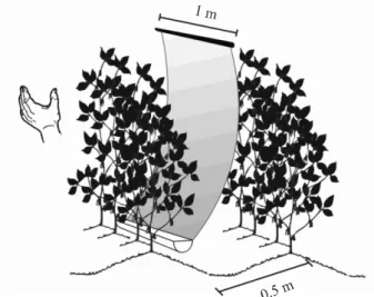
The vertical beat sheet consisted of a wooden stick at the upper end and a 100 mm tube of chlorinated polyvinyl, cut in half lengthwise, at the lower end, connected by a white fabric of 1 m in length, with its height adjusted to that of the soybean plants. The tube served as a collector for the bugs (Figure 1). To collect the bugs, the cloth was placed vertically between the rows of crops, and the plants from just one row were shaken against the surface of the cloth. This procedure was carried out on two metres of the row of soybeans, in order to sample an area of 1 m2.
For each of the 2,156 collections (154 sampling points/phonological stage × 14 phonological stages of the soybean) with an area of 1 m2, the number of stink
bug nymphs and adults were counted for the species
Dichelops furcatus (Fabricius, 1775),Piezodorus guildinii
(Westwood, 1873), Edessa meditabunda (Fabricius,
1794),Nezara viridula (Linnaeus, 1758),Euschistus heros
(Fabricius, 1794) and Chinavia sp. (Say, 1832), thereby
obtaining 12 variables (2 phases x 6 species). Three more variables were then obtained, i.e. the total nymphs, adults and nymphs + adults, for each phonological stage, regardless of species.
Figure 1 - Representation of the vertical beat sheet used for sampling bugs in the soybean crop
Source: Prepared by the authors
sampling points, the following statistics were calculated: minimum, maximum, mean (m), standard deviation (s), variance (s2) and coefficient of variation. Next, the Morisita
index (I ) (MORISITA, 1962) and the k parameter of the negative binomial distribution were calculated employing expressions 1 and 2 respectively:
(1)
(2)
where n is the number of sample points (n = 154), xi is the number of bugs at the ith sampling point, and m is the mean
and s2 the variance of the sample.
The F-test (one-sided) was then applied to the population-density data of the bugs in order to verify the homogeneity of the variances between the two phases of the bug within each combination of species and phenological stage, between the six species within each combination of phase and phenological stage and between the 14 phenological stages of the soybean within each combination of phase and species.
For each of the 15 variables at each phenological stage, taking as a basis the 154 sampling points (n = 154), the sample size was calculated (number of sampling points, ) for the semi-amplitudes of the confidence interval (errors of estimation) equal to 10, 20, 30, 40 and 50% (D) of the estimate of the mean (m) of the population density
of the bugs, expressed as bugs m-2, with a level of
confidence (1- ) of 95%, by means of the expression: =(t2
/2 S2)/(Dm)2 (BUSSAB; MORETTIN, 2004). In
this expression, t/2 is the critical value of the Student’s t-distribution, where the area on the right is equal to /2, i.e. the value of t, such that P (t> t/2) = /2, with (n-1) degrees of freedom, with = 5% probability of error and s2 the
estimation of variance. Then, making equal to 154 sampling points, the error of estimation was calculated as a percentage of the estimate of the mean (m) using expression 3:
(3)
where s is the estimated standard deviation.
Statistical analyses were carried out employing the Microsoft Office Excel ® software with all decimal places being used in the intermediate calculations.
RESULTS AND DISCUSSION
There was variability in the population densities of the bugs for their phases and species and for the phonological stages of the soybeans (Tables 1, 2 and 3). Nymphs were seen in greater quantities than were adults.
Piezodorus guildinii predominated over the other species
of stink bug. Across the phenological stages, population density increased gradually from the initial stages (V7 and V9) to the final stages (R7.1, R7.3 and R8.2), with the peak population of bugs of 19.34 m-2 occurring
for R7.3 (Table 3). These results agree with Silva et al.
(2007) and Mazieroet al. (2009), who showed that during
the reproductive stage of the soybean, the stink-bug population may be made up of more than 70% nymphs compared to adults. A predominance of P. guildinii has
been found in surveys of stink-bug populations in the soybean (LOURENÇÃOet al., 2002). Higher population
densities of the bugs were verified by Belorte, Ramiro and Faria (2003) at stages R7 and R8.
The largest stink-bug infestation occurred during the reproductive stage of the soybean, this phase being the most sensitive to the pest. The bugs colonize during the vegetative phase, but the damage is caused when the bugs feed, starting from the R3 stage of the bean. The decrease in the bug population which occurred in the evaluation that took place in R8.2, can be explained by migration to areas of refuge and the crop no longer being a food preference. Close to the bean harvest, the bugs begin their dispersal to host plants and to diapause niches, in which they remain until the next crop (MEDEIROS; MEGIER, 2009).
In general, the coefficients of variation (CV) of stink-bug population density were higher for the species
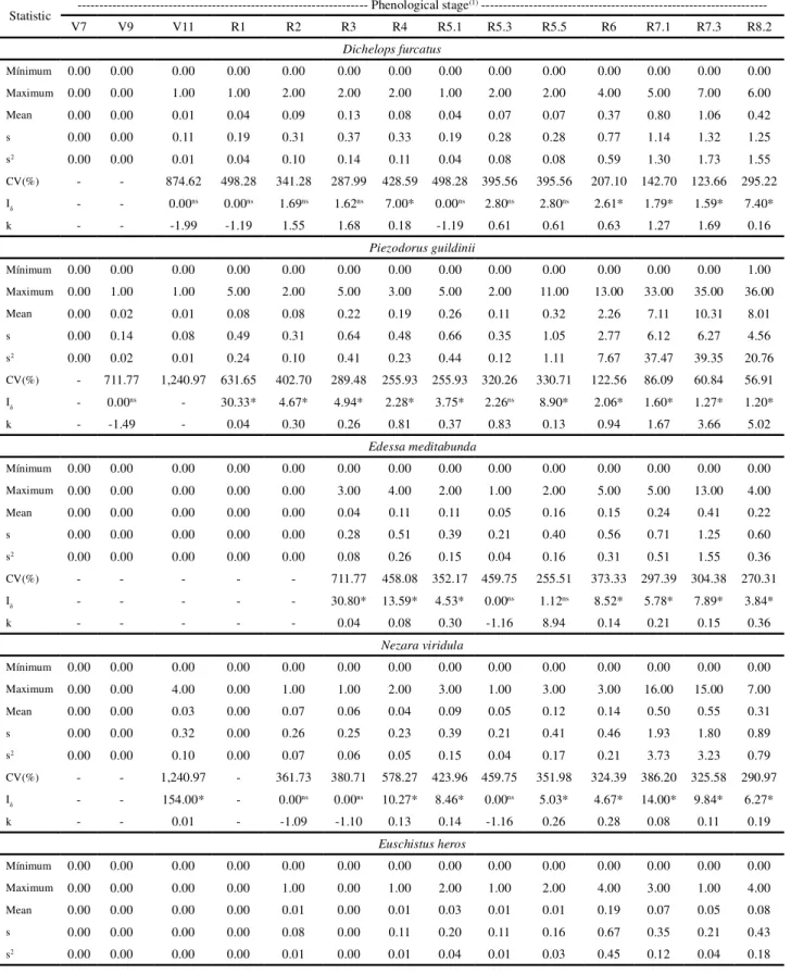
Table 1 - Minimum, maximum, mean, standard deviation (s), variance (s2), coefficient of variation (CV%), Morisita index (I )
and k parameter of the negative binomial distribution, of the population density for nymphs of the stink-bug speciesDichelops
furcatus, Piezodorus guildinii,Edessa meditabunda, Nezara viridula, Euschistus heros andChinavia sp., expressed as stink
bugs m-2, based on 154 points each of 1 m² in area, for 14 phenological stages in the soybean
Statistic --- Phenological stage
(1)
---V7 V9 V11 R1 R2 R3 R4 R5.1 R5.3 R5.5 R6 R7.1 R7.3 R8.2
Dichelops furcatus
Mínimum 0.00 0.00 0.00 0.00 0.00 0.00 0.00 0.00 0.00 0.00 0.00 0.00 0.00 0.00
Maximum 0.00 0.00 1.00 1.00 2.00 2.00 2.00 1.00 2.00 2.00 4.00 5.00 7.00 6.00
Mean 0.00 0.00 0.01 0.04 0.09 0.13 0.08 0.04 0.07 0.07 0.37 0.80 1.06 0.42
s 0.00 0.00 0.11 0.19 0.31 0.37 0.33 0.19 0.28 0.28 0.77 1.14 1.32 1.25
s2 0.00 0.00 0.01 0.04 0.10 0.14 0.11 0.04 0.08 0.08 0.59 1.30 1.73 1.55
CV(%) - - 874.62 498.28 341.28 287.99 428.59 498.28 395.56 395.56 207.10 142.70 123.66 295.22
I - - 0.00ns 0.00ns 1.69ns 1.62ns 7.00* 0.00ns 2.80ns 2.80ns 2.61* 1.79* 1.59* 7.40*
k - - -1.99 -1.19 1.55 1.68 0.18 -1.19 0.61 0.61 0.63 1.27 1.69 0.16
Piezodorus guildinii
Mínimum 0.00 0.00 0.00 0.00 0.00 0.00 0.00 0.00 0.00 0.00 0.00 0.00 0.00 1.00
Maximum 0.00 1.00 1.00 5.00 2.00 5.00 3.00 5.00 2.00 11.00 13.00 33.00 35.00 36.00
Mean 0.00 0.02 0.01 0.08 0.08 0.22 0.19 0.26 0.11 0.32 2.26 7.11 10.31 8.01
s 0.00 0.14 0.08 0.49 0.31 0.64 0.48 0.66 0.35 1.05 2.77 6.12 6.27 4.56
s2 0.00 0.02 0.01 0.24 0.10 0.41 0.23 0.44 0.12 1.11 7.67 37.47 39.35 20.76
CV(%) - 711.77 1,240.97 631.65 402.70 289.48 255.93 255.93 320.26 330.71 122.56 86.09 60.84 56.91
I - 0.00ns - 30.33* 4.67* 4.94* 2.28* 3.75* 2.26ns 8.90* 2.06* 1.60* 1.27* 1.20*
k - -1.49 - 0.04 0.30 0.26 0.81 0.37 0.83 0.13 0.94 1.67 3.66 5.02
Edessa meditabunda
Mínimum 0.00 0.00 0.00 0.00 0.00 0.00 0.00 0.00 0.00 0.00 0.00 0.00 0.00 0.00
Maximum 0.00 0.00 0.00 0.00 0.00 3.00 4.00 2.00 1.00 2.00 5.00 5.00 13.00 4.00
Mean 0.00 0.00 0.00 0.00 0.00 0.04 0.11 0.11 0.05 0.16 0.15 0.24 0.41 0.22
s 0.00 0.00 0.00 0.00 0.00 0.28 0.51 0.39 0.21 0.40 0.56 0.71 1.25 0.60
s2 0.00 0.00 0.00 0.00 0.00 0.08 0.26 0.15 0.04 0.16 0.31 0.51 1.55 0.36
CV(%) - - - 711.77 458.08 352.17 459.75 255.51 373.33 297.39 304.38 270.31
I - - - 30.80* 13.59* 4.53* 0.00ns 1.12ns 8.52* 5.78* 7.89* 3.84*
k - - - 0.04 0.08 0.30 -1.16 8.94 0.14 0.21 0.15 0.36
Nezara viridula
Mínimum 0.00 0.00 0.00 0.00 0.00 0.00 0.00 0.00 0.00 0.00 0.00 0.00 0.00 0.00
Maximum 0.00 0.00 4.00 0.00 1.00 1.00 2.00 3.00 1.00 3.00 3.00 16.00 15.00 7.00
Mean 0.00 0.00 0.03 0.00 0.07 0.06 0.04 0.09 0.05 0.12 0.14 0.50 0.55 0.31
s 0.00 0.00 0.32 0.00 0.26 0.25 0.23 0.39 0.21 0.41 0.46 1.93 1.80 0.89
s2 0.00 0.00 0.10 0.00 0.07 0.06 0.05 0.15 0.04 0.17 0.21 3.73 3.23 0.79
CV(%) - - 1,240.97 - 361.73 380.71 578.27 423.96 459.75 351.98 324.39 386.20 325.58 290.97
I - - 154.00* - 0.00ns 0.00ns 10.27* 8.46* 0.00ns 5.03* 4.67* 14.00* 9.84* 6.27*
k - - 0.01 - -1.09 -1.10 0.13 0.14 -1.16 0.26 0.28 0.08 0.11 0.19
Euschistus heros
Mínimum 0.00 0.00 0.00 0.00 0.00 0.00 0.00 0.00 0.00 0.00 0.00 0.00 0.00 0.00
Maximum 0.00 0.00 0.00 0.00 1.00 0.00 1.00 2.00 1.00 2.00 4.00 3.00 1.00 4.00
Mean 0.00 0.00 0.00 0.00 0.01 0.00 0.01 0.03 0.01 0.01 0.19 0.07 0.05 0.08
s 0.00 0.00 0.00 0.00 0.08 0.00 0.11 0.20 0.11 0.16 0.67 0.35 0.21 0.43
Continuation of Table 1
CV(%) - - - - 1,240.97 - 874.62 755.78 874.62 1,240.97 342.61 483.05 459.75 505.89
I - - - 0.00ns 25.67* 0.00ns 154.00* 7.79* 11.20* 0.00ns 15.79*
k - - - -1.99 0.05 -1.99 0.01 0.15 0.11 -1.16 0.07
Chinaviasp.
Mínimum 0.00 0.00 0.00 0.00 0.00 0.00 0.00 0.00 0.00 0.00 0.00 0.00 0.00 0.00
Maximum 0.00 0.00 0.00 0.00 2.00 2.00 2.00 3.00 5.00 38.00 28.00 14.00 43.00 9.00
Mean 0.00 0.00 0.00 0.00 0.02 0.07 0.10 0.17 0.18 0.52 0.80 1.06 2.08 1.01
s 0.00 0.00 0.00 0.00 0.18 0.28 0.39 0.47 0.58 3.11 3.13 2.10 4.44 1.69
s2 0.00 0.00 0.00 0.00 0.03 0.08 0.15 0.22 0.33 9.70 9.80 4.41 19.72 2.86
CV(%) - - - - 922.54 395.56 402.70 277.61 317.26 599.61 391.86 198.37 213.07 167.02
- - - - 51.33* 2.80ns 7.33* 2.84* 5.70* 35.23* 15.13* 3.99* 5.05* 2.80*
k - - - - 0.03 0.61 0.17 0.56 0.22 0.03 0.07 0.33 0.25 0.55
(1)Developmental stages of the soybean according to Ritchieet al. (1982), adapted by Yorinori (1996). * Morisita index different from 1 by the 2 test at 5%.ns Non-significant. - Not calculated where no stink bugs, or only 1, were found
Statistic --- Phenological state
(1)
---V7 V9 V11 R1 R2 R3 R4 R5.1 R5.3 R5.5 R6 R7.1 R7.3 R8.2
Dichelops furcatus
Mínimum 0.00 0.00 0.00 0.00 0.00 0.00 0.00 0.00 0.00 0.00 0.00 0.00 0.00 0.00
Maximum 1.00 2.00 2.00 1.00 3.00 2.00 3.00 2.00 4.00 3.00 2.00 3.00 5.00 5.00
Mean 0.01 0.08 0.06 0.04 0.05 0.12 0.17 0.13 0.18 0.19 0.05 0.24 0.70 0.72
s 0.08 0.29 0.30 0.19 0.29 0.35 0.47 0.37 0.49 0.50 0.25 0.56 1.11 1.13
s2 0.01 0.09 0.09 0.04 0.08 0.12 0.22 0.14 0.24 0.25 0.06 0.31 1.23 1.29
CV(%) 1,240.97 375.01 454.91 498.28 633.38 283.03 277.61 287.99 270.14 256.35 481.80 233.40 158.17 157.43
I - 2.33ns 6.84* 0.00ns 22.00* 0.90ns 2.84* 1.62ns 2.85* 2.48* 5.50* 2.31* 2.08* 2.09*
k - 0.81 0.19 -1.19 0.06 -10.55 0.56 1.68 0.56 0.70 0.25 0.78 0.93 0.92
Piezodorus guildinii
Mínimum 0.00 0.00 0.00 0.00 0.00 0.00 0.00 0.00 0.00 0.00 0.00 0.00 0.00 0.00
Maximum 2.00 1.00 1.00 2.00 2.00 3.00 2.00 3.00 2.00 3.00 4.00 9.00 19.00 13.00
Mean 0.02 0.02 0.01 0.06 0.13 0.15 0.10 0.19 0.22 0.29 0.31 1.08 3.59 3.80
s 0.18 0.14 0.11 0.26 0.41 0.44 0.33 0.48 0.54 0.63 0.65 1.45 3.21 2.74
s2 0.03 0.02 0.01 0.07 0.17 0.19 0.11 0.23 0.29 0.39 0.43 2.11 10.33 7.53
CV(%) 922.54 711.77 874.62 447.70 313.75 294.33 314.52 255.93 244.26 214.04 209.18 134.81 89.53 72.26
I 51.33* 0.00ns 0.00ns 4.28ns 3.24* 3.04* 1.28ns 2.28* 2.47* 2.18* 2.18* 1.89* 1.52* 1.26*
k 0.03 -1.49 -1.99 0.34 0.47 0.51 3.74 0.81 0.70 0.86 0.86 1.12 1.91 3.86
Edessa meditabunda
Mínimum 0.00 0.00 0.00 0.00 0.00 0.00 0.00 0.00 0.00 0.00 0.00 0.00 0.00 0.00
Maximum 0.00 1.00 0.00 1.00 0.00 1.00 1.00 3.00 1.00 3.00 2.00 2.00 2.00 2.00
Mean 0.00 0.01 0.00 0.01 0.00 0.02 0.03 0.07 0.07 0.08 0.14 0.11 0.18 0.19
s 0.00 0.11 0.00 0.11 0.00 0.14 0.18 0.35 0.26 0.38 0.43 0.37 0.47 0.44
s2 0.00 0.01 0.00 0.01 0.00 0.02 0.03 0.12 0.07 0.14 0.19 0.14 0.22 0.19
CV(%) - 874.62 - 874.62 - 711.77 547.67 483.05 361.73 448.21 304.00 336.60 269.93 233.33
I - 0.00ns - 0.00ns - 0.00ns 0.00ns 11.20* 0.00ns 9.87* 3.33* 3.40* 2.63* 1.14ns
k - -1.99 - -1.99 - -1.49 -1.24 0.11 -1.09 0.12 0.45 0.44 0.63 7.46
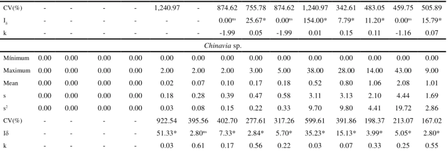
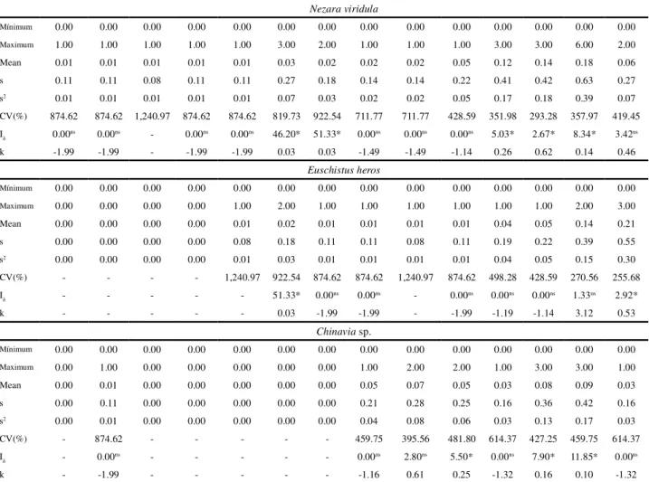
Table 2 - Minimum, maximum, mean, standard deviation (s), variance (s2), coefficient of variation (CV%), Morisita index (I )
and k parameter of the negative binomial distribution, of the population density for adults of the stink-bug speciesDichelops
furcatus, Piezodorus guildinii,Edessa meditabunda, Nezara viridula,Euschistus heros andChinavia sp., expressed as stink
(1)Developmental stages of the soybean according to Ritchieet al. (1982), adapted by Yorinori (1996). * Morisita index different from 1 by the 2 test at 5%.ns Non-significant. - Not calculated where no stink bugs, or only 1, were found
Nezara viridula
Mínimum 0.00 0.00 0.00 0.00 0.00 0.00 0.00 0.00 0.00 0.00 0.00 0.00 0.00 0.00
Maximum 1.00 1.00 1.00 1.00 1.00 3.00 2.00 1.00 1.00 1.00 3.00 3.00 6.00 2.00
Mean 0.01 0.01 0.01 0.01 0.01 0.03 0.02 0.02 0.02 0.05 0.12 0.14 0.18 0.06
s 0.11 0.11 0.08 0.11 0.11 0.27 0.18 0.14 0.14 0.22 0.41 0.42 0.63 0.27
s2 0.01 0.01 0.01 0.01 0.01 0.07 0.03 0.02 0.02 0.05 0.17 0.18 0.39 0.07
CV(%) 874.62 874.62 1,240.97 874.62 874.62 819.73 922.54 711.77 711.77 428.59 351.98 293.28 357.97 419.45
I 0.00ns 0.00ns - 0.00ns 0.00ns 46.20* 51.33* 0.00ns 0.00ns 0.00ns 5.03* 2.67* 8.34* 3.42ns
k -1.99 -1.99 - -1.99 -1.99 0.03 0.03 -1.49 -1.49 -1.14 0.26 0.62 0.14 0.46
Euschistus heros
Mínimum 0.00 0.00 0.00 0.00 0.00 0.00 0.00 0.00 0.00 0.00 0.00 0.00 0.00 0.00
Maximum 0.00 0.00 0.00 0.00 1.00 2.00 1.00 1.00 1.00 1.00 1.00 1.00 2.00 3.00
Mean 0.00 0.00 0.00 0.00 0.01 0.02 0.01 0.01 0.01 0.01 0.04 0.05 0.14 0.21
s 0.00 0.00 0.00 0.00 0.08 0.18 0.11 0.11 0.08 0.11 0.19 0.22 0.39 0.55
s2 0.00 0.00 0.00 0.00 0.01 0.03 0.01 0.01 0.01 0.01 0.04 0.05 0.15 0.30
CV(%) - - - - 1,240.97 922.54 874.62 874.62 1,240.97 874.62 498.28 428.59 270.56 255.68
I - - - 51.33* 0.00ns 0.00ns - 0.00ns 0.00ns 0.00ns 1.33ns 2.92*
k - - - 0.03 -1.99 -1.99 - -1.99 -1.19 -1.14 3.12 0.53
Chinavia sp.
Mínimum 0.00 0.00 0.00 0.00 0.00 0.00 0.00 0.00 0.00 0.00 0.00 0.00 0.00 0.00
Maximum 0.00 1.00 0.00 0.00 0.00 0.00 0.00 1.00 2.00 2.00 1.00 3.00 3.00 1.00
Mean 0.00 0.01 0.00 0.00 0.00 0.00 0.00 0.05 0.07 0.05 0.03 0.08 0.09 0.03
s 0.00 0.11 0.00 0.00 0.00 0.00 0.00 0.21 0.28 0.25 0.16 0.36 0.42 0.16
s2 0.00 0.01 0.00 0.00 0.00 0.00 0.00 0.04 0.08 0.06 0.03 0.13 0.17 0.03
CV(%) - 874.62 - - - 459.75 395.56 481.80 614.37 427.25 459.75 614.37
I - 0.00ns - - - - - 0.00ns 2.80ns 5.50* 0.00ns 7.90* 11.85* 0.00ns
k - -1.99 - - - -1.16 0.61 0.25 -1.32 0.16 0.10 -1.32
Table 3 - Minimum, maximum, mean, standard deviation (s), variance (s2), coefficient of variation (CV%), Morisita index
(I ) and k parameter of the negative binomial distribution for the population density of nymphs, adults, and nymphs and adults of the stink bug, irrespective of speciesDichelops furcatus,Piezodorus guildinii,Edessa meditabunda,Nezara viridula,
Euschistus heros andChinavia sp., expressed as stink bugs m-2, based on 154 points each of 1 m² in area, for 14 phenological
stages in the soybean
Statistic --- Phenological stage
(1)
---V7 V9 V11 R1 R2 R3 R4 R5.1 R5.3 R5.5 R6 R7.1 R7.3 R8.2
Nymphs
Mínimum 0.00 0.00 0.00 0.00 0.00 0.00 0.00 0.00 0.00 0.00 0.00 0.00 1.00 2.00 Maximum 0.00 1.00 4.00 5.00 4.00 5.00 4.00 6.00 5.00 40.00 28.00 34.00 54.00 44.00 Mean 0.00 0.02 0.05 0.12 0.27 0.53 0.53 0.69 0.47 1.19 3.92 9.78 14.47 10.05
s 0.00 0.14 0.35 0.52 0.59 0.89 0.92 1.07 0.83 3.53 4.16 6.92 7.45 5.57
s2 0.00 0.02 0.12 0.27 0.35 0.80 0.84 1.15 0.70 12.47 17.27 47.86 55.54 31.00 CV(%) - 711.77 768.75 447.70 223.32 170.05 174.17 154.65 178.31 295.57 106.12 70.74 51.51 55.39 I - 0.00ns 44.00* 13.08* 2.25* 2.00* 2.14* 1.96* 2.05* 8.89* 1.87* 1.40* 1.20* 1.21*
k - -1.49 0.03 0.09 0.81 1.01 0.88 1.05 0.96 0.13 1.15 2.51 5.10 4.82
(1)Developmental stages of the soybean according to Ritchieet al. (1982), adapted by Yorinori (1996). * Morisita index different from 1 by the 2 test at 5%.ns Non-significant. - Not calculated where no stink bugs, or only 1, were found
Adults
Mínimum 0.00 0.00 0.00 0.00 0.00 0.00 0.00 0.00 0.00 0.00 0.00 0.00 0.00 0.00 Maximum 2.00 2.00 2.00 2.00 3.00 4.00 4.00 6.00 4.00 4.00 5.00 9.00 21.00 14.00 Mean 0.04 0.14 0.08 0.12 0.19 0.34 0.34 0.47 0.57 0.69 0.69 1.71 4.88 5.01
s 0.25 0.36 0.32 0.35 0.54 0.68 0.70 0.86 0.85 0.89 0.94 1.79 3.68 3.07
s2 0.06 0.13 0.10 0.12 0.29 0.46 0.49 0.73 0.72 0.79 0.88 3.21 13.55 9.41 CV(%) 648.47 266.04 381.91 283.03 275.77 197.60 206.58 183.28 148.19 129.22 136.49 104.99 75.47 61.20 I 20.53* 0.73ns 3.95* 0.90ns 3.54* 2.01* 2.32* 2.23* 1.45* 1.22ns 1.41* 1.52* 1.36* 1.17* k 0.06 -3.91 0.37 -10.55 0.40 1.00 0.77 0.82 2.24 4.61 2.44 1.94 2.74 5.71
Nymphs + adults
Mínimum 0.00 0.00 0.00 0.00 0.00 0.00 0.00 0.00 0.00 0.00 0.00 1.00 2.00 5.00 Maximum 2.00 2.00 4.00 5.00 5.00 7.00 6.00 9.00 6.00 40.00 28.00 35.00 56.00 51.00 Mean 0.04 0.16 0.13 0.24 0.46 0.87 0.86 1.16 1.04 1.88 4.60 11.49 19.34 15.06
s 0.25 0.40 0.47 0.63 0.91 1.20 1.24 1.50 1.23 3.58 4.17 7.41 8.42 6.68
s2 0.06 0.16 0.22 0.39 0.83 1.45 1.54 2.24 1.50 12.78 17.42 54.92 70.92 44.56 CV(%) 648.47 255.51 359.78 260.88 197.04 138.25 143.85 128.80 117.95 189.87 90.65 64.51 43.53 44.31 I 20.53* 1.12ns 6.48* 3.70* 2.73* 1.76* 1.91* 1.80* 1.43* 4.06* 1.60* 1.33* 1.14* 1.13*
k 0.06 8.94 0.19 0.38 0.58 1.31 1.10 1.25 2.33 0.33 1.65 3.04 7.26 7.70
Continuation of Table 3
Chinavia sp. compared to those observed forP. guildinii
(Tables 1 and 2). These results suggest that to estimate the average population density ofP. guildinii will require less
sample points. In relation to the phase of the bugs, the higher CV scores for adults suggest the need for a larger sample size compared to that of the nymphs (Tables 1, 2 and 3). These results therefore suggest that sample size varies between the species and stages of the bugs.
The coefficient of variation decreased gradually towards the initial stages (V7 and V9) in relation to the final stages (R7.1, R7.3 and R8.2) (Tables 1, 2 and 3). This behaviour was inversely proportional to that discussed previously for the average population density of stink bugs. These results suggest that to obtain estimates with the same precision, larger sample sizes (number of sampling points) will be needed in the initial stages (larger CVs and lower population densities), with a gradual decrease toward the final stages of the soybean crop (smaller CVs and higher population densities). Moreover, estimates obtained from a single sample size demonstrate less precision in the initial stages and more precision in the final stages.
In practice, the definition of a sample size (number of sampling points) of the desired precision, taken from population densities close to the control level (higher density), is appropriate because it is then the decision is made for the need to control the pest. At lower population densities, it is possible to allow less precision due to the population density being relatively far from the control
level, with the risk of damage being thus lower. As soon as the population of stink bugs increased there was a trend towards homogeneity in the area, resulting in a decrease in the coefficient of variation and consequently fewer sampling points being required when sampling. Similar results were obtained by Cargnelutti Filhoet al. (2011), i.e. the absence
of white grubs at some sampling points (lower population densities) contributed to high coefficients of variation.
In most cases relating to the population density of stink-bug nymphs and adults of the six bug species, and
Table 4 - Variance of population density of stink-bug nymphs and adults of the speciesDichelops furcatus,Piezodorus guildinii,Edessa
meditabunda,Nezara viridula,Euschistus heros andChinavia sp., expressed as stink bugs m-2, based on 154 points each of 1 m² in area,
for 14 phenological stages in the soybean, and values of the F-test for variance homogeneity (F = greater variance/smaller variance)
(1)Developmental stages of the soybean according to Ritchieet al. (1982), adapted by Yorinori (1996). (2) * Variances between the phases of stink bug within each combination of species and phenological stage are heterogeneous by one-sided F test at 5% probability.ns homogeneous variances.(3) * Variance between species within each combination of phase and phenological stage are heterogeneous by one-sided F-test at 5%.(4) * Variances between phenological stages within each combination of phase and species are heterogeneous by one-sided F-test at 5%. - Not calculated where no stink bugs were found
Species Size --- Phenological state
(1)
---V7 V9 V11 R1 R2 R3 R4 R5.1 R5.3 R5.5 R6 R7.1 R7.3 R8.2 F(4)
D. furcatus nymph - - 0.013 0.038 0.096 0.140 0.112 0.038 0.080 0.080 0.588 1.299 1.734 1.553 134.4*
D. furcatus adult 0.006 0.085 0.087 0.038 0.083 0.122 0.220 0.140 0.241 0.249 0.063 0.314 1.230 1.288 198.3*
F(2) - - 6.8* 1.0ns 1.2ns 1.1ns 2.0* 3.7* 3.0* 3.1* 9.4* 4.1* 1.4* 1.2ns
P. guildinii nymph - 0.019 0.006 0.242 0.098 0.408 0.232 0.442 0.125 1.107 7.671 37.471 39.353 20.765 6,060.4*
P. guildinii adult 0.032 0.019 0.013 0.068 0.166 0.193 0.107 0.232 0.291 0.391 0.425 2.112 10.335 7.534 801.0*
F(2) - 1.0ns 2.0* 3.5* 1.7* 2.1* 2.2* 1.9* 2.3* 2.8* 18.0* 17.7* 3.8* 2.8*
E. meditabunda nymph - - - 0.077 0.256 0.151 0.044 0.159 0.311 0.511 1.551 0.356 35.5*
E. meditabunda adult - 0.013 - 0.013 - 0.019 0.032 0.119 0.067 0.143 0.189 0.138 0.224 0.193 17.4*
F(2) - - - - - 4.0* 8.1* 1.3ns 1.5* 1.1ns 1.6* 3.7* 6.9* 1.8*
N. viridula nymph - - 0.104 - 0.067 0.061 0.051 0.149 0.044 0.169 0.215 3.729 3.229 0.789 85.4*
N. viridula adult 0.013 0.013 0.006 0.013 0.013 0.071 0.032 0.019 0.019 0.050 0.169 0.176 0.394 0.074 60.7*
F(2) - - 16.0* - 5.2* 1.2ns 1.6* 7.7* 2.3* 3.4* 1.3ns 21.2* 8.2* 10.6*
E. heros nymph - - - - 0.006 - 0.013 0.039 0.013 0.026 0.445 0.119 0.044 0.182 68.6*
E. heros adult - - - - 0.006 0.032 0.013 0.013 0.006 0.013 0.038 0.050 0.149 0.300 46.2*
F(2) - - - - 1.0ns - 1.0ns 3.0* 2.0* 2.0* 11.8* 2.4* 3.4* 1.6*
Chinavia sp. nymph - - - - 0.032 0.080 0.154 0.220 0.333 9.702 9.796 4.408 19.725 2.863 610.7*
Chinavia sp. adult - 0.013 - - - 0.044 0.080 0.063 0.025 0.130 0.175 0.025 13.5*
F(2) - - - - - - - 5.0* 4.2* 154.9* 384.7* 33.9* 112.9* 112.4*
D. furcatus nymph - - 0.013 0.038 0.096 0.140 0.112 0.038 0.080 0.080 0.588 1.299 1.734 1.553 134.4*
P. guildinii nymph - 0.019 0.006 0.242 0.098 0.408 0.232 0.442 0.125 1.107 7.671 37.471 39.353 20.765 6,060.4*
E. meditabunda nymph - - - 0.077 0.256 0.151 0.044 0.159 0.311 0.511 1.551 0.356 35.5*
N. viridula nymph - - 0.104 - 0.067 0.061 0.051 0.149 0.044 0.169 0.215 3.729 3.229 0.789 85.4*
E. heros nymph - - - - 0.006 - 0.013 0.039 0.013 0.026 0.445 0.119 0.044 0.182 68.6*
Chinavia sp. nymph - - - - 0.032 0.080 0.154 0.220 0.333 9.702 9.796 4.408 19.725 2.863 610.7*
F(3) - - 16.0* 6.4* 15.2* 6.7* 19.8* 11.7* 25.8* 373.5* 45.6* 314.8* 901.1* 113.9*
D. furcatus adult 0.006 0.085 0.087 0.038 0.083 0.122 0.220 0.140 0.241 0.249 0.063 0.314 1.230 1.288 198.3*
P. guildinii adult 0.032 0.019 0.013 0.068 0.166 0.193 0.107 0.232 0.291 0.391 0.425 2.112 10.335 7.534 801.0*
E. meditabunda adult - 0.013 - 0.013 - 0.019 0.032 0.119 0.067 0.143 0.189 0.138 0.224 0.193 17.4*
N. viridula adult 0.013 0.013 0.006 0.013 0.013 0.071 0.032 0.019 0.019 0.050 0.169 0.176 0.394 0.074 60.7*
E. heros adult - - - - 0.006 0.032 0.013 0.013 0.006 0.013 0.038 0.050 0.149 0.300 46.2*
Chinaviasp. adult - 0.013 - - - 0.044 0.080 0.063 0.025 0.130 0.175 0.025 13.5*
F(3) 5.0* 6.6* 13.4* 5.3* 25.6* 10.1* 17.0* 18.0* 44.8* 30.3* 16.7* 42.6* 69.2* 295.9*
(MORISITA, 1962) was higher than one (P 0.05), and the k parameter of the negative binomial distribution tended toward zero (-10.55 k 8.94) (Tables 1, 2 and 3). These results indicate that the stink bugs were distributed as aggregates in the area. When the spatial distribution of insects is aggregate, Cargnelutti Filho et al. (2011)
demonstrated that both the expression presented by Karandinos (1976), commonly used for sample-sizing in the area of entomology, and the expression used in this work give the same estimates of sample size, confirming the suitability of both methods.
The sample size (number of sampling points) in estimating the mean (m) of the population density of stink bugs in combinations of phase and bug species and phenological stage, with the semi-amplitude of the confidence interval equal to 10% of the estimated mean and level of confidence of 95 % , ranged from 127 sampling points (P. guildinii, nymph - R8.2 ) and
60,106 sampling points (P. guildinii, nymph - V11, N. viridula,nymph - V11,E. heros,nymph - R2 and R5.5, D. furcatus, adult - V7,N. viridula, adult - V11 and,adult
- R2 and R5.3 ) (Tables 5 and 6) . In practice, collecting bugs at 60,106 sampling points is difficult. Smaller sample sizes (number of sampling points) have therefore been determined using permitted lower precisions (semi-amplitudes of the confidence interval equal to 20, 30, 40 and 50% of the mean). These sample sizes serve as a basis when planning sampling for specific studies to estimate the mean population density of stink-bug nymphs and adults of the speciesD. furcatus,P. guildinii, E. meditabunda,N. viridula,E. heros andChinaviasp.
for the phenological stages of the soybean. The number of sampling units is dependent on the degree of accuracy required, which varies with the purpose of the research: population dynamics, crop damage, levels of economic loss and pest control (SILVA; COSTA, 1998).
The maximum acceptable error is debateable, leaving the user to choose the desired precision based on the availability of time and labour. Cargnelutti Filhoet al.
(2011) observed that for the estimation of a population of white grubs, the sample size for high accuracy was large and difficult to implement. A large sample size increases the time and cost of sampling, whereas smaller sample sizes can result in less precision, which is also undesirable. It is recommended to use sample sizes that result in high precision while saving time and resources.
To estimate the average population of stink bugs with the same precision, fewer sampling points are needed for the species P. guildinii in relation to the other five
species (Tables 5 and 6). A larger sample size is required for quantification of adult bugs in relation to nymphs (Tables 5, 6 and 7). This difference may be explained by the lower variability ofP. guildinii and of the nymphs respectively.
The nymphs do not display great mobility in the area, because they are devoid of wings. According Fucarinoet al. (2004) the
newly-hatched nymphs remain on the egg mass and only after the third instar do they begin their dispersion.
The sample size obtained was higher for the early and intermediate stages of soybean development, and lower for the final stages (R7.1, R7.3 and R8.2). These results therefore confirm previous inferences that there is variability in the sample size (number of sampling points) when estimating the average population density for the phases and species of stink bug and phenological stages. Employing the net method in the soybean, Costa and Link (1980) found that in larger populations ofP. guildinii andN. viridula,
smaller sizes of sampling unit were defined. Cullen et al. (2000) found that for a greater density ofE. heros
in the tomato, the sample size was smaller. Lúcioet al.
(2009), studying the sample size for mites in the yerba mate, found a variation in the number of samples as a result of the period of evaluation and the degree of pest infestation.
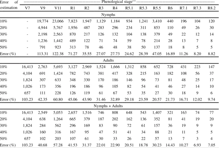
When making a decision about the control of stink bugs in the soybean, it is important to consider the total number of stink bugs. Another aspect to consider is that at population densities close to the control level, quantification should be more accurate, since the wrong estimate at that time can cause a reduction in bean yield. On the other hand, at lower population densities, errors which result in over-estimation are tolerable. Thus, based on the total number of stink bugs (nymphs + adults), the sample size was larger for the initial and intermediate stages of the crop (V7, V9, V11, R1, R2, R3, R4 and R5.1, R5.3 and R5.5), with values ranging between 61 and 1,824 sampling points (error of estimation of 30 %) (Table 7). In the final stages (R6, R7.1, R7.3 and R8.2), the sample sizes which were calculated were smaller and ranged from 9 to 36, which may be explained by the higher population densities of the bugs (between 4.60 and 19.34 bugs m-2) during this
period (Table 3). Thirty-six samples are therefore sufficient when estimating the average population density of stink bugs for these 4 phenological stages when there is a greater incidence of bugs .
Table 5 - Sample size (number of sampling points) to estimate the average population density of stink-bug nymphs of the species
Dichelops furcatus,Piezodorus guildinii,Edessa meditabunda,Nezara viridula,Euschistus heros andChinaviasp., for errors of
estimation equal to 10, 20, 30, 40 and 50 % of the estimated mean and semi-amplitude of the confidence interval (Error %), based on 154 points each of 1 m² in area, for 14 phenological stages
Error of estimation
--- Phenological stage(1)
---V7 V9 V11 R1 R2 R3 R4 R5.1 R5.3 R5.5 R6 R7.1 R7.3 R8.2
Dichelops furcatus
10% - - 29,857 9,691 4,546 3,238 7,170 9,691 6,107 6,107 1,675 795 597 3,402
20% - - 7,465 2,423 1,137 810 1,793 2,423 1,527 1,527 419 199 150 851
30% - - 3,318 1,077 506 360 797 1,077 679 679 187 89 67 378
40% - - 1,867 606 285 203 449 606 382 382 105 50 38 213
50% - - 1,195 388 182 130 287 388 245 245 67 32 24 137
Error (%) - - 139.24 79.32 54.33 45.85 68.23 79.32 62.97 62.97 32.97 22.72 19.69 47.00
Piezodorus guildinii
10% - 19,774 60,106 15,573 6,330 3,271 2,557 2,557 4,004 4,269 587 290 145 127
20% - 4,944 15,027 3,894 1,583 818 640 640 1,001 1,068 147 73 37 32
30% - 2,198 6,679 1,731 704 364 285 285 445 475 66 33 17 15
40% - 1,236 3,757 974 396 205 160 160 251 267 37 19 10 8
50% - 791 2,405 623 254 131 103 103 161 171 24 12 6 6
Error (%) - 113.31 197.56 100.56 64.11 46.08 40.74 40.74 50.99 52.65 19.51 13.71 9.68 9.06
Edessa meditabunda
10% - - - 19,774 8,190 4,841 8,250 2,549 5,440 3,452 3,616 2,852
20% - - - 4,944 2,048 1,211 2,063 638 1,360 863 904 713
30% - - - 2,198 910 538 917 284 605 384 402 317
40% - - - 1,236 512 303 516 160 340 216 226 179
50% - - - 791 328 194 330 102 218 139 145 115
Error (%) - - - 113.31 72.93 56.06 73.19 40.68 59.43 47.34 48.46 43.03
Nezara viridula
10% - - 60,106 - 5,108 5,657 13,052 7,016 8,250 4,836 4,108 5,822 4,138 3,305 20% - - 15,027 - 1,277 1,415 3,263 1,754 2,063 1,209 1,027 1,456 1,035 827
30% - - 6,679 - 568 629 1,451 780 917 538 457 647 460 368
40% - - 3,757 - 320 354 816 439 516 303 257 364 259 207
50% - - 2,405 - 205 227 523 281 330 194 165 233 166 133
Error (%) - - 197.56 - 57.59 60.61 92.06 67.49 73.19 56.03 51.64 61.48 51.83 46.32
Euschistus heros
10% - - - - 60,106 - 29,857 22,295 29,857 60,106 4,582 9,107 8,250 9,989
20% - - - - 15,027 - 7,465 5,574 7,465 15,027 1,146 2,277 2,063 2,498
30% - - - - 6,679 - 3,318 2,478 3,318 6,679 510 1,012 917 1,110
40% - - - - 3,757 - 1,867 1,394 1,867 3,757 287 570 516 625
50% - - - - 2,405 - 1,195 892 1,195 2,405 184 365 330 400
Error (%) - - - - 197.56 - 139.24 120.32 139.24 197.56 54.54 76.90 73.19 80.54
Chinavia sp.
10% - - - - 33,218 6,107 6,330 3,008 3,929 14,033 5,994 1,536 1,772 1,089
20% - - - - 8,305 1,527 1,583 752 983 3,509 1,499 384 443 273
30% - - - - 3,691 679 704 335 437 1,560 666 171 197 121
40% - - - - 2,077 382 396 188 246 878 375 96 111 69
50% - - - - 1,329 245 254 121 158 562 240 62 71 44
Table 6 - Sample size (number of sampling points) to estimate the average population density of stink-bug adults of the species
Dichelops furcatus,Piezodorus guildinii,Edessa meditabunda,Nezara viridula,Euschistus heros andChinaviasp., for errors
of estimation equal to 10, 20, 30, 40 and 50 % of the estimated mean and semi-amplitude of the confidence interval (Error %), based on 154 points each of 1 m² in area, for 14 phenological stages
Error of estimation
--- Phenological stage(1)
---V7 V9 V11 R1 R2 R3 R4 R5.1 R5.3 R5.5 R6 R7.1 R7.3 R8.2
Dichelops furcatus
10% 60,106 5,489 8,077 9,691 15,658 3,127 3,008 3,238 2,849 2,565 9,061 2,127 977 968
20% 15,027 1,373 2,020 2,423 3,915 782 752 810 713 642 2,266 532 245 242
30% 6,679 610 898 1,077 1,740 348 335 360 317 285 1,007 237 109 108
40% 3,757 344 505 606 979 196 188 203 179 161 567 133 62 61
50% 2,405 220 324 388 627 126 121 130 114 103 363 86 40 39
Error (%) 197.56 59.70 72.42 79.32 100.83 45.06 44.20 45.85 43.01 40.81 76.70 37.16 25.18 25.06
Piezodorus guildinii
10% 33,218 19,774 29,857 7,823 3,843 3,382 3,861 2,557 2,329 1,789 1,708 710 313 204
20% 8,305 4,944 7,465 1,956 961 846 966 640 583 448 427 178 79 51
30% 3,691 2,198 3,318 870 427 376 429 285 259 199 190 79 35 23
40% 2,077 1,236 1,867 489 241 212 242 160 146 112 107 45 20 13
50% 1,329 791 1,195 313 154 136 155 103 94 72 69 29 13 9
Error (%) 146.87 113.31 139.24 71.27 49.95 46.86 50.07 40.74 38.88 34.07 33.30 21.46 14.25 11.50
Edessa meditabunda
10% - 29,857 - 29,857 - 19,774 11,707 9,107 5,108 7,841 3,608 4,422 2,844 2,125
20% - 7,465 - 7,465 - 4,944 2,927 2,277 1,277 1,961 902 1,106 711 532
30% - 3,318 - 3,318 - 2,198 1,301 1,012 568 872 401 492 316 237
40% - 1,867 - 1,867 - 1,236 732 570 320 491 226 277 178 133
50% - 1,195 - 1,195 - 791 469 365 205 314 145 177 114 85
Error (%) - 139.24 - 139.24 - 113.31 87.19 76.90 57.59 71.35 48.40 53.59 42.97 37.15
Nezara viridula
10% 29,857 29,857 60,106 29,857 29,857 26,227 33,218 19,774 19,774 7,170 4,836 3,358 5,002 6,867 20% 7,465 7,465 15,027 7,465 7,465 6,557 8,305 4,944 4,944 1,793 1,209 840 1,251 1,717 30% 3,318 3,318 6,679 3,318 3,318 2,915 3,691 2,198 2,198 797 538 374 556 763 40% 1,867 1,867 3,757 1,867 1,867 1,640 2,077 1,236 1,236 449 303 210 313 430 50% 1,195 1,195 2,405 1,195 1,195 1,050 1,329 791 791 287 194 135 201 275 Error (%) 139.24 139.24 197.56 139.24 139.24 130.50 146.87 113.31 113.31 68.23 56.03 46.69 56.99 66.78
Euschistus heros
10% - - - - 60,106 33,218 29,857 29,857 60,106 29,857 9,691 7,170 2,858 2,552
20% - - - - 15,027 8,305 7,465 7,465 15,027 7,465 2,423 1,793 715 638
30% - - - - 6,679 3,691 3,318 3,318 6,679 3,318 1,077 797 318 284
40% - - - - 3,757 2,077 1,867 1,867 3,757 1,867 606 449 179 160
50% - - - - 2,405 1,329 1,195 1,195 2,405 1,195 388 287 115 103
Error (%) - - - - 197.56 146.87 139.24 139.24 197.56 139.24 79.32 68.23 43.07 40.70
Chinavia sp.
10% - 29,857 - - - 8,250 6,107 9,061 14,732 7,125 8,250 14,732
20% - 7,465 - - - 2,063 1,527 2,266 3,683 1,782 2,063 3,683
30% - 3,318 - - - 917 679 1,007 1,637 792 917 1,637
40% - 1,867 - - - 516 382 567 921 446 516 921
50% - 1,195 - - - 330 245 363 590 285 330 590
Error (%) - 139.24 - - - 73.19 62.97 76.70 97.81 68.02 73.19 97.81
Table 7 - Sample size (number of sampling points) to estimate the average population density of stink-bug nymphs, adults, and nymphs and adults, irrespective of speciesDichelops furcatus,Piezodorus guildinii,Edessa meditabunda,Nezara viridula,Euschistus heros
andChinaviasp., for errors of estimation equal to 10, 20, 30, 40 and 50 % of the estimated mean and semi-amplitude of the confidence
interval (Error %), based on 154 points each of 1 m² in area, for 14 phenological stages
(1)Developmental stages of the soybean according to Ritchieet al. (1982), adapted by Yorinori (1996). - Not calculated where no stink bugs were found
Error of estimation
--- Phenological stage(1)
---V7 V9 V11 R1 R2 R3 R4 R5.1 R5.3 R5.5 R6 R7.1 R7.3 R8.2
Nymphs
10% - 19,774 23,066 7,823 1,947 1,129 1,184 934 1,241 3,410 440 196 104 120
20% - 4,944 5,767 1,956 487 283 296 234 311 853 110 49 26 30
30% - 2,198 2,563 870 217 126 132 104 138 379 49 22 12 14
40% - 1,236 1,442 489 122 71 74 59 78 214 28 13 7 8
50% - 791 923 313 78 46 48 38 50 137 18 8 5 5
Error (%) - 113.31 122.38 71.27 35.55 27.07 27.73 24.62 28.39 47.05 16.89 11.26 8.20 8.82
Adults
10% 16,413 2,763 5,693 3,127 2,969 1,524 1,666 1,312 858 652 728 431 223 147
20% 4,104 691 1,424 782 743 381 417 328 215 163 182 108 56 37
30% 1,824 307 633 348 330 170 186 146 96 73 81 48 25 17
40% 1,026 173 356 196 186 96 105 82 54 41 46 27 14 10
50% 657 111 228 126 119 61 67 53 35 27 30 18 9 6
Error (%) 103.23 42.35 60.80 45.06 43.90 31.46 32.89 29.18 23.59 20.57 21.73 16.71 12.02 9.74 Nymphs + Adults
10% 16,413 2,549 5,053 2,657 1,516 746 808 648 543 1,407 321 163 74 77
20% 4,104 638 1,264 665 379 187 202 162 136 352 81 41 19 20
30% 1,824 284 562 296 169 83 90 72 61 157 36 19 9 9
40% 1,026 160 316 167 95 47 51 41 34 88 21 11 5 5
50% 657 102 203 107 61 30 33 26 22 57 13 7 3 4
Error (%) 103.23 40.68 57.28 41.53 31.37 22.01 22.90 20.51 18.78 30.23 14.43 10.27 6.93 7.05
Any integrated pest management in the soybean requires that planning be based on solid foundations, such as the diagnosis of the species of bug, identification and registering of age throughout the crop cycle, and above all, the quantification of the number of individuals present in the cultivated areas. Thus, a correct, accurate and speedy quantification of the population of pentatomidae in the soybean is the only indicator that can determine the actions necessary for control, and is therefore the way to protect the crop from losses in production, with lesser costs and lower environmental impact.
Knowing the exact number of sampling points in order to obtain the average population density of stink bugs is therefore the first step when planning, followed by carrying out sampling in the field and diagnosis of the population density, which will indicate to producers, technical assistants and administrators the correct time to make the decision about management.
CONCLUSION
There is variability in the sample size (number of sampling points) when estimating the average population density of stink bugs, between the phases and species of the bugs and between the phenological stages of the soybean. Smaller sample sizes are needed for the nymphs of P. guildinii and final phonological
stages (R6, R7.1, R7.3 and R8.2) compared to the adults of D. furcatus,E. meditabunda, N. viridula,E. heros andChinavia sp. and the initial (V7, V9 and V11)
ACKNOWLEDGEMENTS
The authors wish to thank the National Council for Scientific and Technological Development (CNPq) and the Coordination for the Improvement of Higher Education Personnel (CAPES), for the grant of a scholarship to the authors. Thanks are also due to the scholarship students and volunteers for their assistance in collecting the data.
REFERENCES
BELORTE, L. C. C; RAMIRO, Z. A.; FARIA, A. M. Levantamento de percevejos pentatomídeos em cinco cultivares de soja [Glycine max(L.) Merrill, 1917] na região de Araçatuba, SP.Arquivos do
Instituto Biológico, v. 70, n. 4, p. 447-451, 2003.
BUSSAB, W. O.; MORETTIN, P. A.Estatística básica. 5. ed. São Paulo: Saraiva, 2004. 526 p.
CARGNELUTTI FILHO, A. et al. Dimensionamento de
amostra na estimação da população de corós em áreas de campo nativo e de cultivo no Estado do Rio Grande do Sul.Ciência Rural, v. 41, n. 8, p. 1300-1306, 2011.
COMPANHIA NACIONAL DE ABASTECIMENTO. 2011.
Disponível em: <http://www.conab.gov.br/OlalaCMS/uploads/ arquivos/11_11_09_15_03_02_boletim_2o_levantamento_ safra_2011_12.pdf>. Acesso em: 11 abr. 2012.
CORRÊA-FERREIRA, B. S. Suscetibilidade da soja a percevejos na fase anterior ao desenvolvimento das vagens. Pesquisa Agropecuária Brasileira, v. 40, n. 11, p. 1067-1072, 2005.
CORRÊA-FERREIRA; B. S.; AZEVEDO, J. de. Soybean seed damage by different species of stink bugs. Agricultural and Forest Entomology, v. 4, n. 2, p. 145-150, 2002.
COSTA, E. C.; LINK, D. Determinação do tamanho da unidade amostral para o método da rede, em soja, para insetos de importância agrícola.Revista do Centro de Ciências Rurais, v. 10, n. 2, p. 115-123, 1980.
CULLEN, E. M. et al. Quantifying trade-offs between pest
sampling time and precision in commercial IPM sampling programs.Agricultural Systems, v. 66, n. 2, p. 99-113, 2000.
FUCARINO, A.et al. Chemical and physical signals mediating
conspecific and heterospecific aggregation behavior of first instar stink bugs.Journal of Chemical Ecology, v. 30, n. 6, p. 1257-1269, 2004.
GUEDES, J. V. C. et al. Capacidade de coleta de dois
métodos de amostragem de insetos-praga da soja em diferentes espaçamentos entre linhas.Ciência Rural, v. 36, n. 4, p. 1299-1302, 2006.
GUEDES, J. V. C.et al. Percevejos da soja: novos cenários, novo manejo.Revista Plantio Direto, v. 12, n. 1, p. 24-30, 2012.
KARANDINOS, M. G. Optimal sample size and comments on some published formulae. Bulletin of the Entomological Society of America, v. 22, n. 4, p. 417-421, 1976.
LOURENÇÃO, A. L.et al. Avaliação de danos de percevejos e de desfolhadores em genótipos de soja de ciclos precoce, semiprecoce e médio.Neotropical Entomology, v. 31, n. 4, p. 623-630, 2002.
LÚCIO, A. D. C. et al. Distribuição espacial e tamanho de
amostra para o ácaro-do-bronzeado da erva-mate. Revista Árvore, v. 33, n. 1, p. 143-150, 2009.
MAZIERO, H. et al. Volume de calda e inseticidas no
controle de Piezodorus guildinii (Westwood) na cultura da
soja.Ciência Rural, v. 39, n. 5, p. 1307-1309, 2009.
MEDEIROS, L.; MEGIER, G. A. Ocorrência e desempenho de
Euschistus heros (F.) (Heteroptera: Pentatomidae) em plantas
hospedeiras alternativas no Rio Grande do Sul. Neotropical Entomology, v. 38, n. 4, p. 459-463, 2009.
MORISITA, M. Id-index, a measure of dispersion of individuals. Researches on Population Ecology, v. 4, n. 1, p. 01-07, 1962.
RITCHIE, S. W. et al. How a soybean plant develops.
Ames: Iowa State University of Science And Technology Cooperative Extension Service, 1982.
EMPRESA BRASILEIRA DE PEQUISA AGROPECUÁRIA. Indicações técnicas para a cultura da soja no Rio Grande do Sul e em Santa Catarina 2010/2011 e 2011/2012. Cruz Alta: Fundacep Fecotrigo, 2010. 168 p.
SANTOS, R. S. S. dos. Levantamento populacional de percevejos e da incidência de parasitóides de ovos em cultivos orgânicos de soja.Pesquisa Agropecuária Gaúcha, v. 14, n. 1, p. 41-46, 2008.
SILVA, M. T. B. daet al. Erro e resistência.Revista Cultivar:
Grandes Culturas, v. 9, n. 82, p. 22-25, 2007.
SILVA, M. T. B.; COSTA, E. C. Tamanho e número de unidades de amostra de solo para amostragem de larvas de
Diloboderus abderus (Sturm) (Coleoptera: Melolonthidae)
em plantio direto. Anais da Sociedade Entomológica do Brasil, v. 27, n. 2, p. 193-197, 1998.
STÜRMER, G. R.et al. Eficiência de métodos de amostragem de lagartas e de percevejos na cultura de soja.Ciência Rural, v. 42, n. 12, p. 2105-2111, 2012.