Triple-Filter Core Inflation: A Measure
of the Inflation Trajectory
P
EDRO
C
OSTA
F
ERREIRA
∗
D
AIANE
M
ARCOLINO DE
M
ATTOS
†
V
AGNER
L
AERTE
A
RDEO
‡
Contents: 1. Introduction; 2. An analysis of the core measures disclosed in Brazil; 3. Trend Measure: Triple-Filter Core inflation; 4. Results; 5. Final Remarks. Keywords: CPI; Core inflation; Smoothed trimmed mean; Moving average; Seasonal
adjustment.
JEL Code: C13, E31, E52.
In countries with high inflation, as is the case of Brazil, the traditional cores inflation do not seem to deliver much information about the general level of prices. Therefore, we present a new measure, the Triple-Filter core inflation, which filters inflation in three ways: trimmed mean with smoothed items, seasonal adjustment and moving averages. The results allow us to say that the Triple-Filter core inflation, in addition to providing more information about the inflation trajectory than traditional core inflation, provides a more up-to-date view on the state of inflation than the accumulated inflation over 12 months.
Em países com inflação elevada, como é o caso do Brasil, os núcleos tradicionais não parecem trazer muita informação sobre o nível geral dos preços. Portanto, apresenta-se uma nova medida, o Núcleo Triplo Filtro, que filtra a inflação de três maneiras: médias aparadas com suavização, ajuste sazonal e médias móveis. Os resultados permitem dizer que o núcleo triplo filtro, além de trazer mais informação a respeito da trajetória da inflação do que os núcleos tradicionais, fornece uma visão mais atual sobre o estado da inflação do que a inflação.
1. INTRODUCTION
The core inflation measures are used by monetary authorities as a tool to measure the stabilization of prices in the economy. Despite being a popular term among policymakers, there is still no consensus on its definition nor on what it plans to capture. The consensus is that the change in the price level, despite being a monetary phenomenon, can be influenced also by non-monetary events such as, for example, bad weather conditions that make food prices more expensive because of a reduced supply of these products to the population. However, since this event is temporary, with an improving climate food prices may fall again. This transient behavior thus adds noise to the inflation rate and, therefore, the monetary authorities should be able to distinguish between a transient effect and a persistent effect on the price level when making their decisions. Given this, an inflation measure free of such interference is desirable.
A measure of inflation free of such noise, which aims to show the persistent price movement or, in other words, the inflation trend, can be understood as the core inflation (Bryan and Cecchetti, 1994). Thus, efforts are directed to identify and remove such noise of aggregate inflation. In the 1970s, the core was understood as inflation after removing the food and energy components (CPI less food and energyof the United States), precisely because they are very volatile components. Over time, however, several other authors suggested ways of removing the noise from the rate of inflation. Bryan and Cecchetti (1994), for example, suggested estimators of limited influence (median and trimmed inflation) to calculate inflation. Such estimators are more robust to extreme variations that add noise to inflation, and allow a more satisfactory measure for the persistent component of inflation as compared to the core excluding the food and energy items. Dow (1994) suggested not to delete any price calculation but to recalculate its weight in proportion to the inverse of its volatility (double weight). So very volatile items have low weight in the calculation of the core inflation. In 2002, Cogley showed that the cores estimated by methods already cited still preserved high frequency variations and therefore suggested an exponential smoothing-based method that returned a measure of inflation softer than the alternative measures. There are still other estimated cores for other statistical models, such as Quah and Vahey (1995), that used multivariate systems in terms of other macro-economic variables to extract the trend of inflation and Bradley et al. (2015) and Stock and Watson (2015), who used models of unobservable components to estimate the core.
As can be seen, there are different methods that allow an estimation of the trend of inflation. How-ever, the construction of a core alone does not guarantee its usefulness, and, on this basis, scholars have proposed methods to qualify the performance of these measures (Wynne, 1999, Clark, 2001, Rich and Steindel, 2007). Generally, the following characteristics in a core inflation are expected: (a)Low volatility: it is expected that the core is less volatile than the aggregate inflation; (b)Transparency and communication with the public: it is desirable that the core is easy to replicate and to explain to the public, making the presentation of the core dialogue simpler. As shown Da Silva Filho and Figueiredo (2014), most core inflations disclosed by central banks in the world are of the exclusion, double weight or trimmed mean types. Few institutions have more complex statistical methods to calculate the core, and if such are presented, also disclose the simplest core inflation; (c)Historical review: it is expected that the measure does not require an historical review, that is, does not change the past or its tendency with the insertion of new data. This makes a consistent history of inflation counted using the core in-flation; (d)Capture the inflation trend: according to Clark (2001), for a core measure to capture the trend of inflation, the core and headline inflation should present similar means, ensuring that the core does not overestimate or underestimate the long-term trend of inflation, and the trajectory of the core must follow closely the headline inflation trend. Thus, when the trend of inflation rises, so will the core. The procedures applied for the evaluation of these two criteria can be found in more detail in Clark (2001), Cogley (2002), Rich and Steindel (2007); (e)Inflation forecasting: It is also expected the core will help in inflation forecasts, although the literature shows that this is not a trivial task. However, some authors (Clark, 2001, Cogley, 2002, Rich and Steindel, 2007) used a simple linear regression to assess whether the difference between the core and the headline inflation in the current time helps predict how much headline inflation will change from the current time to a few months from now.
Several of these authors say there is no consensus on which is the best measure of core inflation since the core does not present all of the expected characteristics (usually the items (a) and (d)) and therefore recommend the use of a set of indicators with caution, knowing the capacity of each to extract information. These findings corroborate the reason central banks do not disclose only a single measure of core and also not lean on just a single tool for decision making.
This paper is structured as follows: in the next section is an analysis of the core measures disclosed in Brazil, mainly checking the five expected core criteria. Section 3 presents the proposed methodology, that is, how the Triple-Filter core inflation is calculated. Section 4, in addition to presenting the pro-posed measure, compares it with the conventional core measures especially in showing the ability of the Triple- Filter core to capture the trajectory of the headline inflation and provide information about the current state of the general level of prices. Finally, section 5 has the final considerations.
2. AN ANALYSIS OF THE CORE MEASURES DISCLOSED IN BRAZIL
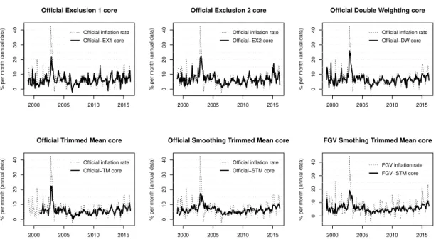
Currently, there are six core inflation measures disclosed in Brazil. Five of them are estimated by the Central Bank of Brazil (BCB) and have reference to the IPCA,1the official rate of inflation in the country
estimated by IBGE (2016b). The other measure refers to the CPI,2 estimated by IBRE (2016a) of the
Getulio Vargas Foundation (FGV). The measures3 vary from Jan/1999 to Mar/2016 and are shown in
Figure 1. It is easy to see that all preserve a lot of noise in their history, with the trimmed mean core softer in the field but still suggesting indications of seasonality.
Figure 1: Core for the IPCA (IBGE) and the CPI (FGV/IBRE)−Jan/1999 to Mar/2016 (annual data)
Official Exclusion 1 core
% per month (ann
ual data)
2000 2005 2010 2015
0
10
20
30
40 Official inflation rate Official−EX1 core
Official Exclusion 2 core
% per month (ann
ual data)
2000 2005 2010 2015
0
10
20
30
40 Official inflation rate Official−EX2 core
Official Double Weighting core
% per month (ann
ual data)
2000 2005 2010 2015
0
10
20
30
40 Official inflation rate Official−DW core
Official Trimmed Mean core
% per month (ann
ual data)
2000 2005 2010 2015
0
10
20
30
40 Official inflation rate Official−TM core
Official Smoothing Trimmed Mean core
% per month (ann
ual data)
2000 2005 2010 2015
0
10
20
30
40 Official inflation rate Official−STM core
FGV Smothing Trimmed Mean core
% per month (ann
ual data)
2000 2005 2010 2015
0
10
20
30
40 FGV inflation rate FGV−STM core
To understand and analyze the trajectory of inflation in Brazil, however, these cores should be less noisy and also without seasonality (seasonal test,4available in Table 1, suggests, with 95% confidence,
the existence of a seasonal component in all core measures), as this component can mask the real trajec-tory of a time series. But despite this, these cores may still be suitable with regard to the characteristics desirable in view in section 1. The assessment of such measures is made ahead.
1The Broad Consumer Price Index (IPCA) (IBGE, 2016a). 2The Consumer Price Index (CPI) (IBRE, 2016b).
3Official-EX1: Core for the IPCA that excludes monitored items and food at home; Official-EX2: Core for the IPCA which
excludes the ten most volatile items; Official-DW: Core for the IPCA using double weighting method; Official-TM: Core for the IPCA using trimmed mean; Official-STM: Core for the IPCA using trimmed mean method with smoothed items; FGV-STM: Core for the CPI using trimmed mean method with smoothed items.
Table 1: QS Seasonality Test
qs-stat p-value
Official-EX1 21.65 0.0000 Official-EX2 28.57 0.0000 Official-DW 10.12 0.0063 Official-TM 7.08 0.0290 Official-STM 12.27 0.0021 FGV-STM 28.11 0.0000
H0: There is no seasonality in time series.
Table 2 displays descriptive statistics for the six core measures. All measurements have lower vari-ability to the reference inflation index, highlighting the trimmed mean cores. It is noteworthy that all cores also have an average lower than the inflation rate, indicating they underestimate the long-term trend of price variation, and this average difference is more pronounced for the trimmed mean Official Brazilian CPI (Official-TM) and for the smoothed single core released by FGV (FGV-STM). This difference is mitigated when considering only the ten most recent years of information, however, it still represents a high bias around 1 percentage point for these two last mentioned cores. The Official-DW is the core that has a lower bias, however, one of the highest variability. The cores by exclusion are the ones in which the bias is not significant when assessing the most recent ten years. Except for this, all cores are classified as biased to the historical average of inflation.
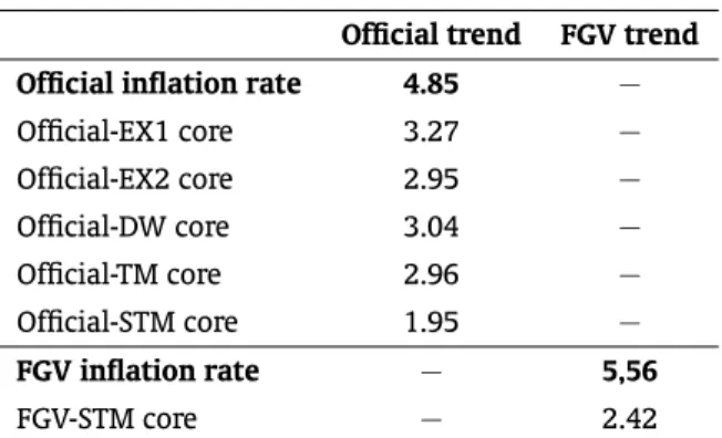
Table 3 presents the RMSE (Root Mean Square Error) between the core measures and the long-term trend of inflation, the latter obtained by the centered moving average for 36 months on the reference in-flation index. Centered moving averages are often used to estimate the trend of a time series, however, it is important to pay attention to the fact that the most recent period, which is the most interesting to assess the inflation trajectory, cannot be rated due to the loss of the most recent information in the calculation. The cores that demonstrate the lowest RMSE, among the whole set of measures, are the two core inflations by trimmed mean with smoothed items: Official-STM and FGV-STM.
Table 2: Descriptive statistics and evaluation of bias to the core inflations measures of Brazil
Mean Median Standard Deviation Bias p-value Official inflation rate 7.02 (6.07) 6.29 (5.79) 5.23 (3.55) − − Official-EX1 6.15 (5.89) 5.54 (5.41) 3.28 (2.95) -0.86 (-0.18) 0.01 (0.19) Official-EX2 6.65 (5.84) 6.17 (5.66) 3.53 (2.78) -0.37 (-0.23) 0.00 (0.23)
Official-DW 6.76 (6.01) 6.29 (5.91) 3.47 (2.19) -0.26 (-0.06) 0.00 (0.00)
Official-TM 5.71 (5.11) 5.28 (5.03) 2.98 (2.11) -1.31 (-0.96) 0.00 (0.00)
Official-STM 6.47 (5.77) 6.17 (5.54) 2.46 (1.78) -0.55 (-0.30) 0.00 (0.00)
FGV inflation rate 6.90 (6.11) 6.42 (5.98) 6.00 (4.75) − −
FGV-STM 5.66 (5.05) 5.28 (4.97) 2.81 (1.98) -1.24 (-1.07) 0.00 (0.00)
In addition to the proximity of trends, it is also necessary to verify whether the core has a long-term relationship with inflation, that is, it is expected that when the inflation trend increase (decreases), the core also increases (decreases). To verify this relationship you need to apply the following unit root and cointegration tests. The ADF unit root test (Table 4) applied to the entire series (Jan/1999 to Mar/2016) suggests that some measures are stationary, for example, Official inflation rate and CPI (FGV inflation rate). However, the same test applied only to the ten most recent years (values in parentheses in the same table), indicates that all measures are considered as a stochastic trend with a 95% confidence level, indicating the lack of inflation stability in Brazil during this recent period. Based on the results for these two time horizons, it was considered that the series are not stationary. The ADF test was reapplied to all the differentiated measures and results, with 95% confidence, indicating that they are stationary.
Table 3: RMSE between trend inflation and cores
Official trend FGV trend
Official inflation rate 4.85 −
Official-EX1 core 3.27 − Official-EX2 core 2.95 −
Official-DW core 3.04 −
Official-TM core 2.96 −
Official-STM core 1.95 −
FGV inflation rate − 5,56
FGV-STM core − 2.42
Note: the statistics were obtained based on annualized measures.
Table 4: Augmented Dickey & Fuller Test
τ-stat Critical Value Lag Conclusion
Official inflation rate -3.929 (0.262) -2.88 (-1.95) 07 (09) rejectH0(do not rejectH0) Official-EX1 -2.237 (-2.364) -2.88 (-2.88) 11 (11) do not rejectH0(do not rejectH0) Official-EX2 -2.737 (-2.169) -2.88 (-2.88) 13 (08) do not rejectH0(do not rejectH0) Official-DW -3.486 (0.133) -2.88 (-1.95) 07 (13) rejectH0(do not rejectH0) Official-TM -3.126 (1.085) -2.88 (-1.95) 07 (15) rejectH0(do not rejectH0) Official-STM -2.149 (1.546) -2.88 (-1.95) 12 (10) do not rejectH0(do not rejectH0) FGV inflation rate -3.096 (1.032) -2.88 (-1.95) 12 (14) rejectH0(do not rejectH0) FGV-STM -2.290 (3.044) -2.88 (-1.95) 12 (11) do not rejectH0(do not rejectH0)
H0: There is unit root (time series is not stationary). Figures in parenthesis are calculated considering the history of Apr/2006 to Mar/2016 (ten years), while others consider the historical series starting in Jan/1999.
Table 5: Johansen Cointegration Test.
Eigenvalue Test
Statistic Critical Value
No. of cointegration
equations Conclusion
Official inflation rate & Official-EX1 core
0.077 15.52 14.26 None rejectH0
0.025 5.00 3.84 At most 1 rejectH0
Two cointegrating equations at the 5% level.
Official inflation rate & Official-EX2 core
0.198 44.94 14.26 None rejectH0
0.089 18.89 3.84 At most 1 rejectH0
Two cointegrating equations at the 5% level.
Official inflation rate & Official-DW core
0.097 20.24 14.26 None rejectH0
0.069 14.22 3.84 At most 1 rejectH0
Two cointegrating equations at the 5% level.
Official inflation rate & Official-TM core
0.209 41.60 14.26 None rejectH0
0.080 14.90 3.84 At most 1 rejectH0
Two cointegrating equations at the 5% level.
Official inflation rate & Official-STM core
0.142 29.79 14.26 None rejectH0
0.017 3.48 3.84 At most 1 do not rejectH0 One cointegrating equation at the 5% level.
FGV inflation rate & FGV-STM core
0.237 54.09 14.26 None rejectH0
0.031 6.27 3.84 At most 1 rejectH0
Two cointegrating equations at the 5% level.
∆πt=α+λµt−1+
p
X
k=1
αk∆πt−k+εt (1)
∆πtc=α+λcµt−1+
p
X
k=1
αk∆πtc−k+εt (2)
where:
πc
tis the core inflation (annualized monthly percent change);
µt−1is the cointegration vector, which comes down toπt−πtcif the core is unbiased;
∆ = 1−Lin which L is the lag operator such thatLnyt=yt−n.
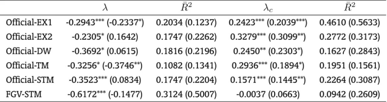
As there is supposedly a long-term relationship for all measures, the adjustment dynamics can be assessed. The evaluation is made in the analysis of the coefficientsλandλcof the equations (1) and (2)
(Mehra and Reilly, 2009), indicating how the inflation and the core adjust when there is some difference between them. It is expected thatλis negative andλcis zero, so we can conclude that inflation moves
towards the core and the core does not move toward inflation.
The results shown in Table 6 suggest that the adjustment dynamic is given appropriately only for the FGV-STM core, that is, it can be concluded that only inflation moves towards the core and not the other way (λsignificant and negative andλcnot significant). However, the same analysis for the ten
most recent years (figures in brackets in Table 6) does not suggest the expected dynamic for any of the measures. In some cases, for example Official-EX1 and Official-TM cores, the dynamic occurs in two possible ways: the core moves toward inflation (λcsignificant) and inflation moves towards the core (λ
significant and negative).
Table 6: Dynamic between inflation and core inflation – Jan/1999 to Mar/2016
λ R¯2 λ
c R¯2
Official-EX1 -0.2943*** (-0.2337*) 0.2034 (0.1237) 0.2423*** (0.2039***) 0.4610 (0.5633) Official-EX2 -0.2305* (0.1642) 0.1747 (0.2262) 0.3279*** (0.3099**) 0.2772 (0.3173) Official-DW -0.3692* (0.0615) 0.1816 (0.2196) 0.2450** (0.2303*) 0.1627 (0.2843) Official-TM -0.3256* (-0.3746**) 0.1082 (0.1341) 0.2936*** (0.1894*) 0.1951 (0.1561) Official-STM -0.3523*** (0.0834) 0.1747 (0.2204) 0.1571*** (0.1445**) 0.2264 (0.3087) FGV-STM -0.6172*** (-0.1477) 0.3124 (0.5007) -0.0037 (0.0663) 0.0942 (0.2609) Note: significance levels: 5% (*), 1% (**) e 0.1% (***).
The statistics were obtained based on annualized measures. Figures in parenthesis are calculated considering the history of Apr/2006 to Mar/2016 (ten years), while others consider the historical series starting in Jan/1999.
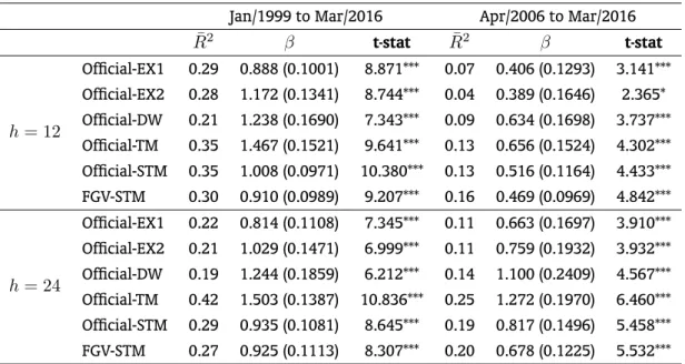
In order to verify whether the difference between the core and the inflation in the current time (t) helps predict inflation in 1 and 2 years (t+ 12andt+ 24), it was estimated using the equation (3).
πt+h−πt=α+β(πct−πt) +εt (3)
where:
πtis the inflation rate (annualized monthly percent change);
πc
tis the core inflation (annualized monthly percent change).
ahead (adjustedR2equals 25%). Although the values are relatively low, by the simplicity of the model, such values are acceptable and are also useful to compare the performance of the cores between them.
Table 7: Forecasting inflation rate using core inflation
Jan/1999 to Mar/2016
Apr/2006 to Mar/2016
¯
R
2β
t-stat
R
¯
2β
t-stat
h
= 12
Official-EX1
0.29
0.888 (0.1001)
8.871***
0.07
0.406 (0.1293)
3.141***
Official-EX2
0.28
1.172 (0.1341)
8.744***
0.04
0.389 (0.1646)
2.365*
Official-DW
0.21
1.238 (0.1690)
7.343***
0.09
0.634 (0.1698)
3.737***
Official-TM
0.35
1.467 (0.1521)
9.641***
0.13
0.656 (0.1524)
4.302***
Official-STM
0.35
1.008 (0.0971)
10.380***
0.13
0.516 (0.1164)
4.433***
FGV-STM
0.30
0.910 (0.0989)
9.207***
0.16
0.469 (0.0969)
4.842***
h
= 24
Official-EX1
0.22
0.814 (0.1108)
7.345***
0.11
0.663 (0.1697)
3.910***
Official-EX2
0.21
1.029 (0.1471)
6.999***
0.11
0.759 (0.1932)
3.932***
Official-DW
0.19
1.244 (0.1859)
6.212***
0.14
1.100 (0.2409)
4.567***
Official-TM
0.42
1.503 (0.1387)
10.836***
0.25
1.272 (0.1970)
6.460***
Official-STM
0.29
0.935 (0.1081)
8.645***
0.19
0.817 (0.1496)
5.458***
FGV-STM
0.27
0.925 (0.1113)
8.307***
0.20
0.678 (0.1225)
5.532***
Note:βstandard deviation in parenthesis; t-stat is the test statistic ofβparameter.
With the results presented, we conclude that no core inflation measure has optimum performance when considering all the analyzed criteria. All core inflations underestimate the inflation trend, and this is the most expressive feature in the cores inflation by trimmed mean, however these are less noisy than the Official-EX1, Official-EX2 and Official-DW cores inflation, which underestimate less. All the measures also have a long-term relationship with inflation, but this relationship does not occur properly for any of them, except for the FGV-STM. However, this ratio can also be questioned because the ability to attract inflation is considered a failure for the most recent period of data. The forecast capacity is most relevant for the trimmed mean cores inflation, although it can be questionable in the most recent period.
In view of this, it is worth the effort to find another measure of core inflation that satisfies the criteria used in this study.
3. TREND MEASURE: TRIPLE-FILTER CORE INFLATION
Viewing the analysis in section 2, we notice the poor performance of the currently disclosed core infla-tions in Brazil, and the trimmed mean with smoothed items are the ones that stand out when consider-ing bias, forecast, adjustment dynamics and proximity of the aggregated inflation. Similar conclusions can be found in other studies of the core measures in Brazil (Da Silva Filho and Figueiredo, 2011, Santos and Castelar, 2013, Da Silva Filho and Figueiredo, 2014). Because of this, three procedures are suggested in order to improve the performance of a core by smoothing trimmed mean and find a trend measure for inflation:
2. Remove the identified seasonality;
3. Apply a short filter of moving averages to remove the high frequency component remaining after seasonal adjustment.
The smoothing trimmed mean core inflation excludes from the price index the items with the high-est and lowhigh-est variations in the period. So, every month it is decided whether an item remains or is excluded from the index calculation. By using smoothing, it allows that some items have a chance to not be summarily excluded. For example, administered items that have less frequent adjustments, but at significant times. Smoothing divides the variation of these predefined items in 12 and also distributes in a 12-month horizon. The smoothed items account for about 37% of the FGV inflation basket.5
Changing the number of items that will be removed from the core calculation is intended to ap-proximate the average of the core inflation to the average of the headline inflation, eliminating the average bias. Removal of the seasonal component is important to avoid misinterpretation regarding the time series trend. To deseasonalize the series, the seasonal adjustment program X-13ARIMA-SEATS (U.S. Census Bureau, 2013) was used. However, even with seasonal adjustment, a time series may still be considered volatile, precisely because the purpose of seasonal adjustment is only to remove the sea-sonal component and not the high frequency component (irregular/noise). Economic analysts generally use smoothing techniques to try to capture the supposed tendency of a volatile time series, such as, for example, moving averages. If there is seasonality in the time series, usually the order 12 is used (variation accumulated in 12 months) or higher to analyze the trajectory of inflation (as is done in Brazil). The downside here is that the current inflation is very affected by past values. In this article, however, after removal of seasonality, one can employ a moving average of short order (three months) for the purpose of removing only high-frequency variations. Thus, current inflation is little influenced by the past (equation (4)). After these three filters (extreme variations, seasonality, noise), there is the (annualized) Triple-Filter core inflation (TF core inflation).
πT Fi,t =
2 Y
i=0 πAJ
i,t−i
100 + 1 !
12 3
−1
×100. (4)
Where: πAJ
i,t is the core inflation seasonally adjusted (monthly percent change);
πT F
i,t is the annualized Triple-Filter core.
The methodology presented will be applied only to the FGV inflation rate (CPI) but can be easily replicated for any consumer price index. The first filtering methodology excludes items with extreme variations that accumulate 20% of the lower tail and 13% of the upper tail, leaving 67% of the original weight of the basket of products. The estimation made by FGV/IBRE considers 20% for the two tails. The seasonally adjusted specifications (second filter) were set considering the complete historical series from January 1999 to March 2016. Two outliers were detected (Feb/1999 and Nov/2002), which were kept to perfect the quality of seasonal adjustment. The SARIMA(0 1 1)(1 0 0)12model was estimated taking into account the raw data.
5The items that are smoothed in the trimmed mean methodology are: Residential Rental, Residential Housing, Residential
4. RESULTS
4.1. The Triple-Filter core inflation and its characteristics
The TF core inflation, shown in Figure 2, is the estimated trend measure for the CPI (FGV/IBRE) following the procedures seen in the section 3. Clearly, the measure is less volatile than the price index and note that its trajectory is increasing from 2010, whereupon the indicator floats around the inflation target ceiling (6.5%) stipulated by the Central Bank, reaching beyond it significantly from 2014. The latest available data (2016) point to a possible stabilization and even decrease of the price trend.
Figure 2: TF core inflation of CPI (FGV/IBRE) - Mar/1999 a Mar/2016 (annual data)
% per month (ann
ual data)
2000 2005 2010 2015
0
10
20
30
40 FGV inflation rate (CPI)
TF core inflation Inflation Target Tolerance interval
Furthermore, the analysis of the TF core inflation (Table 8) allows us to conclude that the measure is not biased (p-value = 0.58), that is, the core inflation does not underestimate or overestimate the inflation trend. The conclusion is also valid when analyzing the ten most recent years (p = 0.29). These first positive results were achieved after the new definition of the number of items with extreme variations that should be excluded in calculating the trimmed mean methodology.
When measuring the distance between the TF core inflation and the price trend obtained by the moving averages (Table 9), this distance can be considered small compared to the core inflation now published by FGV/IBRE (FGV-STM), concluding that, on average, the TF core inflation follows the infla-tion trend closer than the current FGV core inflainfla-tion.
Table 8: Descriptive statistics and evaluation of bias to the Triple-Filter core inflation
Table 9: RMSE between FGV trend inflation and Triple-Filter core
FGV trend
FGV-STM 2,42
TF core inflation 1,41
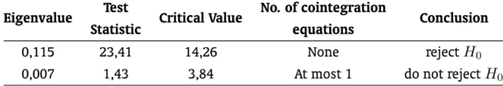
It is also possible to conclude that the TF core inflation and the inflation trend have a long-term relationship because, with 95% confidence, the two time series are first order integrated (Table 10) and cointegrated (Table 11). The dynamics of this long-term relationship between the TF core inflation and the CPI is given as expected (see Table 12). Sinceλis negative and significant, when inflation is above or below the core inflation, it will tend to move towards the core inflation. There is no evidence of the opposite movement (core toward inflation), sinceλcis not significant. This dynamic is maintained
when evaluating the ten most recent years of data. These results together demonstrate that the TF core inflation captures the inflation trend properly.
Table 10: Augmented Dickey & Fuller Test
τ-stat Critical Value Lag Conclusion
FGV inflation rate -3.096 -2.88 12 rejectH0 FGV inflation rate (recent) 1.032 -1.95 14 do not rejectH0 TF core inflation -1.982 -2.88 16 do not rejectH0 TF core inflation (recent) 1.852 -1.95 18 do not rejectH0
H0: There is unit root (time series is not stationary).
ADF test is applied considering the history of Mar/1999 to Mar/2016 and the ten most recent years of data.
Table 11: Johansen Cointegration Test between IPC and Triple-Filter core
Eigenvalue Test
Statistic Critical Value
No. of cointegration
equations Conclusion
0,115 23,41 14,26 None rejectH0
0,007 1,43 3,84 At most 1 do not rejectH0 One cointegrating equation at the 5% level.
Table 12: Dynamic between CPI and Triple-Filter core inflation
λ R¯2
λc R¯2
TF core inflation -1.925*** 0.4372 -0.0021 0.5885 TF core inflation (recent) -0.515*** 0.5392 0.005 0.2851
Note: significance levels: 0.1% (***)
The dynamic is evaluated considering the history of Mar/1999 to Mar/2016 and the ten most recent years data.
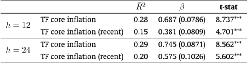
Table 13: Forecasting inflation rate using core inflation
¯ R2
β t-stat
h= 12 TF core inflation 0.28 0.687 (0.0786) 8.737*** TF core inflation (recent) 0.15 0.381 (0.0809) 4.701***
h= 24 TF core inflation 0.29 0.745 (0.0871) 8.562*** TF core inflation (recent) 0.20 0.575 (0.1026) 5.602***
Note:βstandard deviation in parenthesis; t-stat is the test statistic ofβparameter.
4.2. New analyzes
Also it is necessary to assess whether over time the TF core inflation trajectory remains similar to adding new observations, since seasonal adjustment is used. For this evaluation, we adopted the following:
1. Setting the specification of seasonal adjustment model considering only the data until Dec 2014; 2. Run the seasonal adjustment month-to-month from Jan 2015 to Mar 2016 according to the
speci-fication defined in (1) and store the result of each month;
3. Deseasonalize the full range according to the specification defined in (1) and compare it with the number obtained in (2).
The annualized TF core inflation series obtained from the two previously explained ways can be seen in Figure 3. Note that from 2014 there is a small change between the two series. This change is most evident in the months of January and February 2016, in which the difference between the series is, respectively, 0.5 and 0.4 percentage points (with annualized information). Except in the months of March and April 2015 wherein the estimated core inflation with the complete series moves from 8.5% to 8.6% while the other core inflation recedes from 8.4% to 8.3%, the trajectory of the core inflations is similar. These results show the robustness of the proposed core inflation and that the seasonal adjust-ment month-to-month is similar when using all the observations of the series available. This result and others (softness, bias, cointergration, adjustment dynamic, seasonal robustness and prediction) shown in this section show the quality of the measure of the core inflation proposal.
Figure 3: Evaluation of seasonal adjustment (annual data)
% per month (ann
ual data)
2000 2005 2010 2015
4 6 8 10 12 14
all data month−to−month
passes it three times in February, March and November, however, the accumulated inflation only came to exceed the ceiling for the first time in May 2014.
Figure 4: Annualized TF core inflation and 12-month cumulative CPI – Mar/1999 a Mar/2016
% per month (ann
ual data)
2000 2005 2010 2015
0
5
10
15
20
12−month cumulative CPI TF core inflation Inflation Target Tolerance interval
These results demonstrate that the TF core inflation should be used as a reference measure for the inflation path in place of the traditional core inflations, especially in countries with higher inflation and regulated prices, as is the case of Brazil. In this context, the traditional core inflations bring little information about the trajectory of the general price level, so the argument of simplicity in the core inflation calculation is not valid like it is in countries like the US who only remove energy and food from the estimate.
allowing the public to have a clearer idea about the behavior of prices over a full year without having to carry a significant load of information from 12 months ago (a common practice in countries with high inflation is accumulating inflation over 12 months). Significant, because the core inflation also carries the past 12 months of information, however variations are softer due to the smoothing methodology in the calculation of trimmed mean and are applied to only 37% of the basket of products. It is important that the property of the TF core inflation to save little past information allows a variation in the clearest tip to events occurring at the present time.
Such features previously argued (clearer trend, improved communication, clearer view with what happens in the present time) are easily confirmed observing the history of the TF core inflation and relating it to the events in Brazil. By comparing Figures 1 and 2, it is easy to see that the tendency of the TF core inflation is lighter and less volatile as compared with traditional cores. As for annualization and improved communication, observing Figure 2, there are three events that support this argument. It appears that since 2003 there is a clear convergence of inflation to the target, achieved in 2006, and inflation remains on target to approximately the end of 2010. From this period, inflation measured by the core inflation touches the target ceiling until January 2014, when the goal is not met.
The third characteristic is observed when comparing the TF core inflation over 12 months (Figure 4), where it appears that the behavior of the accumulated inflation is perceived faster with TF core inflation. It can be argued that the policymakers use other techniques besides the accumulated inflation in 12 months and therefore have full knowledge of price movements. However, in Brazil, the main tool used by the general public to assess where inflation is at the present time is the accumulated inflation over 12 months, and this, by definition, carries with it a large amount of past information, which may not reflect the current price situation. Therefore, the TF core inflation will allow the general public to have a more accurate understanding of the trend of prices allowing greater vigilance to short-term movements of price increase and, on the other hand, a smaller effort from the Central Bank to decrease price levels and, in the future, may serve as an anchor in the dissemination process for the Brazilian society in general.
5. FINAL REMARKS
The core inflation measures are used by monetary authorities as a tool to measure the stabilization of prices in the economy. Such measures try to capture the persistant inflation movement by removing the short term moviments in the CPI. In Brazil, the five existing core measures, which are estimated by using traditional methods, deliver little information in respect to general price levels. That is why this article seeks to estimate a new core measure: the Triple-Filter core inflation method which is built by filtering the CPI by trimmed mean with smoothed items, seasonal adjustment and moving averages.
The results (softness, no bias, cointergration, adjustment dynamic, seasonal robustness and predic-tion) show the quality of the measure of the core inflation proposal and allow above all to conclude that this can be more useful to identify the current pricing trend than traditional measures. The measure allows the general public to have a more accurate understanding of the trend of prices allowing greater vigilance to short-term movements of price increase and, on the other hand, a smaller effort from the Central Bank to decrease price levels and, in the future, may serve as an anchor in the dissemination process for the Brazilian society in general.
BIBLIOGRAPHY
Bradley, M. D., Jansen, D. W., & Sinclair, T. M. (2015). How Well Does “Core” Inflation Capture Permanent Price Changes? Macroeconomic Dynamics, 19(4):791–815.
Bryan, M. F. & Cecchetti, S. G. (1994). Measuring core inflation. InMonetary Policy. The University of Chicago Press, p. 195–219.
Clark, T. E. (2001). Comparing measures of core inflation.Federal Reserve Bank of Kansas City - Economic Review, Q II:5–31.
Cogley, T. (2002). A simple adaptive measure of core inflation. Journal of Money, Credit and Banking, 34:94–113.
Da Silva Filho, T. N. T. & Figueiredo, F. M. R. (2011). Has Core Inflation Been Doing a Good Job in Brazil? Revista Brasileira de Economia, 65:207–233.
Da Silva Filho, T. N. T. & Figueiredo, F. M. R. (2014). Revisitando as Medidas de Núcleo de Inflação do Banco Central do Brasil. Banco Central do Brasil - Trabalhos para Discussão, 356.
Dow, J. (1994). Measuring inflation using multiple price indexes. [Mimeo].
Ferreira, P., Oliveira, I., & Teixeira, F. (2016). How Brazilian Consumers Inflation Expectations are created. [Mimeo].
Gaglianone, W. P., Issler, J. V., & Matos, S. M. (2016). Applying a Microfounded-Forecasting Approach to Predict Brazilian Inflation. Banco Central do Brasil - Working Paper, 436.
IBGE (2016a). Índice Nacional de Preços ao Consumidor Amplo – IPCA e Índice Nacional de Preços ao Consumidor – INPC. Online at: ❤tt♣✿✴✴✇✇✇✳✐❜❣❡✳❣♦✈✳❜r✴❤♦♠❡✴❡st❛t✐st✐❝❛✴✐♥❞✐❝❛❞♦r❡s✴ ♣r❡❝♦s✴✐♥♣❝❴✐♣❝❛✴❞❡❢❛✉❧t✐♥♣❝✳s❤t♠.
IBGE (2016b). Instituto Brasileiro de Geografia e Estatística. Online at:❤tt♣✿✴✴✇✇✇✳✐❜❣❡✳❣♦✈✳❜r.
IBRE (2016a). Instituto Brasileiro de Economia. Online at:❤tt♣✿✴✴♣♦rt❛❧✐❜r❡✳❢❣✈✳❜r✴.
IBRE (2016b). Instituto Brasileiro de Economia - IPC. Online at:❤tt♣✿✴✴♣♦rt❛❧✐❜r❡✳❢❣✈✳❜r✴♠❛✐♥✳ ❥s♣❄❧✉♠❈❤❛♥♥❡❧■❞❂✹✵✷✽✽✵✽✶✶❉✽❊✸✹❇✾✵✶✶❉✾✷❇✼✸✺✵✼✶✵❈✼.
Mehra, Y. P. & Reilly, D. (2009). Short-Term Headline-Core Inflation Dynamics. Federal Reserve Bank of Richmond Economic Quarterly, p. 289–313.
Quah, D. & Vahey, S. P. (1995). Measuring Core Inflation? Economic Journal, 105(432):1130–44.
Rich, R. & Steindel, C. (2007). A Comparison of Measures of Core Inflation. Federal Reserve Bank of New York Economic Policy Review, 13:19–38.
Santos, C. & Castelar, I. (2013). Avaliando as medidas de núcleo da inflação no Brasil.Associação Nacional dos Centros de Pós-Graduação em Economia.
Stock, J. H. & Watson, M. W. (2015). Core Inflation and Trend Inflation. Working Paper 21282, National Bureau of Economic Research.
U.S. Census Bureau (2013). The X-13ARIMA-SEATS Seasonal Adjustment Program. Online at: ❤tt♣s✿ ✴✴✇✇✇✳❝❡♥s✉s✳❣♦✈✴sr❞✴✇✇✇✴①✶✸❛s✴.